Power-Law Distributions from Sigma-Pi Structure of Sums of Random Multiplicative Processes
by
Arthur Matsuo Yamashita Rios de Sousa
1,*, 
Hideki Takayasu
2,3,
Didier Sornette
2,4,5 and
Misako Takayasu
1,2 1
Department of Mathematical and Computing Science, School of Computing, Tokyo Institute of Technology, Yokohama 226-8502, Japan
2
Institute of Innovative Research, Tokyo Institute of Technology, Yokohama 226-8502, Japan
3
Sony Computer Science Laboratories, Tokyo 141-0022, Japan
4
Department of Management, Technology and Economics, ETH Zürich, Zürich 8092, Switzerland
5
Swiss Finance Institute, University of Geneva, Geneva 1211, Switzerland
*
Author to whom correspondence should be addressed.
Entropy 2017, 19(8), 417; https://doi.org/10.3390/e19080417
Submission received: 2 August 2017
/
Revised: 13 August 2017
/
Accepted: 16 August 2017
/
Published: 17 August 2017
(This article belongs to the Special Issue Statistical Mechanics of Complex and Disordered Systems)
Abstract
:We introduce a simple growth model in which the sizes of entities evolve as multiplicative random processes that start at different times. A novel aspect we examine is the dependence among entities. For this, we consider three classes of dependence between growth factors governing the evolution of sizes: independence, Kesten dependence and mixed dependence. We take the sum X of the sizes of the entities as the representative quantity of the system, which has the structure of a sum of product terms (Sigma-Pi), whose asymptotic distribution function has a power-law tail behavior. We present evidence that the dependence type does not alter the asymptotic power-law tail behavior, nor the value of the tail exponent. However, the structure of the large values of the sum X is found to vary with the dependence between the growth factors (and thus the entities). In particular, for the independence case, we find that the large values of X are contributed by a single maximum size entity: the asymptotic power-law tail is the result of such single contribution to the sum, with this maximum contributing entity changing stochastically with time and with realizations.
1. Introduction
Power-laws appear in the probability distributions of many physical systems and human activities, being one of the signatures of complex systems [1,2]. Usually occurring in its tail, i.e., for sufficiently large events, a probability density function of a random variable x with this behavior is such that:
A probability distribution with a power-law tail is characterized by a much slower decay compared with an exponential law, and thus large events may not be negligible. Another distinctive and unique property of power-laws is that they obey the symmetry of scale invariance: the functional form of the distribution remains unchanged under a scale transformation. In addition, for these distributions, the moments of order larger than or equal to diverge [3,4].
The frequent observation of power-law distributions in natural and social systems as well as their interesting mathematical properties have motivated the search for mechanisms that generate power-laws [3,5,6]. One of the first proposed power-law generation mechanisms, which is recurrently applied to model a diversity of phenomena, is “proportional growth”, also known in network theory as “preferential attachment”. In this mechanism, a quantity is distributed among existing entities according to probabilities proportional to the quantity they already possess, establishing a “rich get richer” dynamics [7,8,9]. Another iconic conceptual framework is self-organized criticality, captured by the metaphor of avalanches in a sandpile, in which power-laws are spontaneous emergent properties, with no apparent need to adjust control parameters [10,11]. Among many other mechanisms, let us mention the superposition of probability distributions [12,13], formalized in the concept of superstatistics [14,15,16]; the key idea is that the basic non-power-law probability distribution of a system has parameters that are random variables themselves and, when including this second source of stochasticity, a power-law distribution may arise. A particular case of superstatistics that found wide applicability is the Tsallis statistics, where the extremization of its generalized entropy produces power-laws [17].
An additional relevant model for generating power-law distributions is the class of random multiplicative processes, often used to model growth of entities, such as business firms, cities, and biological populations [18,19,20,21,22,23,24,25]. The common starting point to explain the mechanisms of power-law formation in those growth phenomena is the Gibrat’s law of proportional growth, stating that an entity grows proportionally to its current size but with a growth rate independent of it [26]. This law leads to the basic random multiplicative process expressed in discrete times:
where is the size of entity at time t, represents the multiplicative factor and the discrete time growth rate is equal to .
However, the Gibrat’s law alone cannot explain a power-law distribution since the corresponding process (2) produces a non-stationary log-normal distribution, considering independent and identically distributed random variables with finite mean and variance. To obtain a power-law tail, it is necessary to assure a contraction tendency and add some kind of surviving mechanism to the basic random multiplicative process. The simplest manifestation of such mechanisms is the introduction of an additive term to the process, leading to stochastic multiplicative affine processes, also often referred to as the Kesten process [27,28,29,30,31]:
with being the additive term. Another related surviving mechanism is the inclusion of the additive term only when the system crosses a lower threshold, acting as a barrier preventing the collapse to zero [32]. Under general conditions, when those ingredients are added to the basic random multiplicative process, a power-law tailed distribution is obtained.
Here, we propose a simple growth model that combines basic random multiplicative processes with the idea of superposition of distributions mentioned above. The superposition of distributions has a neat interpretation: it corresponds to considering entities that are born successively. Combining the features of birth and stochastic proportional growth has been considered in [23,33,34]. Our model can be viewed as the simplest and purest incarnation of these mechanisms. This allows us to examine dependence among entities in three particular different classes: complete independence; Kesten dependence (a dependence based on the Kesten process); and mixed dependence, combining both independence and Kesten dependence. Rather than studying the cross-section at a given time of the sizes of entities present in the system (as done, e.g., in [23,33,34]), we study the distribution of the sum of sizes of all entities in the system. This corresponds to the total capitalization of a country, when entities are firms, or to the total biomass of an ecosystem for biological populations. We obtain a random variable whose structure takes the form of a sum of product terms. As a result of this structure, its distribution has a power-law tail with the same exponent regardless of the dependence type—indicating a common general ingredient for power-laws—but with distinct tail formation mechanisms resulting from the degree of dependence among entities.
2. Model Description and Formal Solution
2.1. Model Definition
Consider a set of entities of sizes . At each time step, the sizes of existing entities evolve as basic random multiplicative processes and one new entity is born with unit size. The size of a given entity j at time t is defined as:
By definition, the time of birth of a given entity is its index j minus 1. Thus, the first entity with index is born (of unit size) at time . The factors are identically distributed random variables. Here, we take positive half-normally distributed random variables with variance , i.e., , with normally distributed: .
The quantity that we study is the sum of the sizes of all existing entities present in the system at time t, excluding the last entity born at t that has index and size :
By recursion, the size of entity j at time t is given by:
Then, the sum of entity sizes reads:
The first sum in the right side of expression (7) is over all the t entities that have been born until time t (excluding the last one, as mentioned above). For a given entity j, the product term is made of growth factors corresponding to the number of time periods of stochastic proportional growth allowed by its age.
2.2. Dependence Structure of the Growth Factors
The entities are not necessarily independent. External factors can influence more than one entity at the same time, resulting in dependence between the growth rates for different entities. For instance, there could exist situations in which such that . In this work, from the numerous possible dependence types, we examine the following three particular ones:
- Independence: all entities are growing independently:Observe that the notation does not mean that these variables cannot have by chance the same value. This notation just expresses that they are independent random variables.
- Kesten dependence: external influences determine the same growth factor for all existing entities at each given time, but the growth factor is a random variable as a function of time. This case reproduces the solution of the Kesten process (3) and constitutes a novel interpretation of the said process, originally representing a single entity evolving in the presence of an additive term:
- Mixed dependence: alternation between independence and Kesten dependence, say independence for odd t and Kesten dependence for even t, representing a time-changing dependence. Note that this is only one of the many possibilities for the combination of independence and Kesten dependence.
Regardless of the dependence type, the solution for the sum of sizes has the structure of a sum of increasing products of random variables, which we refer to as Sigma-Pi:
We have changed into (compare with (7)) as this gives the same number and structure of terms, when summed over j from 1 to n. As mentioned before, the identically distributed random variables are not necessarily all independent and their interdependence characterizes the dependence type.
2.3. Asymptotic Power-Law Tails
This Sigma-Pi structure has received special attention in the context of the Kesten process. For Kesten dependence, letting , the central result [27] states that, provided that the multiplicative factors are contracting on average (, where the notation stands for the expected operator and log, for the natural logarithm), ensuring stationarity, the distribution of X presents a power-law tail behavior, with the complementary cumulative distribution function of X, , behaving as:
where C is called the “scale factor” and the exponent is determined by the relation (provided that there is a solution ):
Then, for half-normally distributed random variables, , Equation (12) shows that is uniquely determined by , where the explicit relationship is conveniently expressed by as a function of [35]:
It has been shown rigorously that the power-law asymptotic result (11) with (12) also applies for the independence case [36] (this fact was first suggested by the authors, as acknowledged in [36]), up to a logarithmic correction so that . In fact, we conjecture that the result (11) with (12), up to slowly varying functions multiplying the scale factor C, holds for any dependence type with the restriction that all variables in a product term are independent (see Appendix A), or more generally with a sufficiently weak dependence. In other words, the sizes of the entities can be interdependent via the action of common simultaneous growth factors, but the growth factors themselves should exhibit no (or just a weak) dependence along the time dimension. We thus expect a power-law distribution with the same exponent for all three particular cases made explicit above: independence, Kesten dependence and mixed dependence. This conjecture is tested numerically in the next section.
2.4. Generalization
We end this section by commenting that the addition of more realistic ingredients to the model, such as random birth rates and the inclusion of stochastic deaths of the entities, can be represented by the generalized Sigma-Pi of the form:
where the coefficients depend on the details of the modified model. For instance, the death of some entity j that occurred at some time between its birth and the “present time” n amounts to take . We indicate in Appendix A that, for a large class of coefficients , result (11) with (12) still holds. Intuitively, this is because the behavior of given by (14) is controlled asymptotically by just a few terms in the sum, or by the single largest term only, depending on the dependence structure. Interpreted for a system, the total system size is thus controlled by few entities.
3. Numerical Simulations and Discussion
3.1. Numerical Construction of the Complementary Cumulative Distribution Function of Sum of Sizes
In this section, we check numerically the prediction (11) with (12) for the complementary cumulative distribution function of the random variable (7) or equivalently (10) in the limit of large t or n. Numerically, we have used two methods to generate the set of to construct : (i) recording the successive values of over time n and (ii) constructing thousands of independent ensembles of time evolutions of and recording all the values of this ensemble at a fixed time. We have checked (see Appendix B) that the two methods yield the same results, supporting the validity of the ergodicity property for the process .
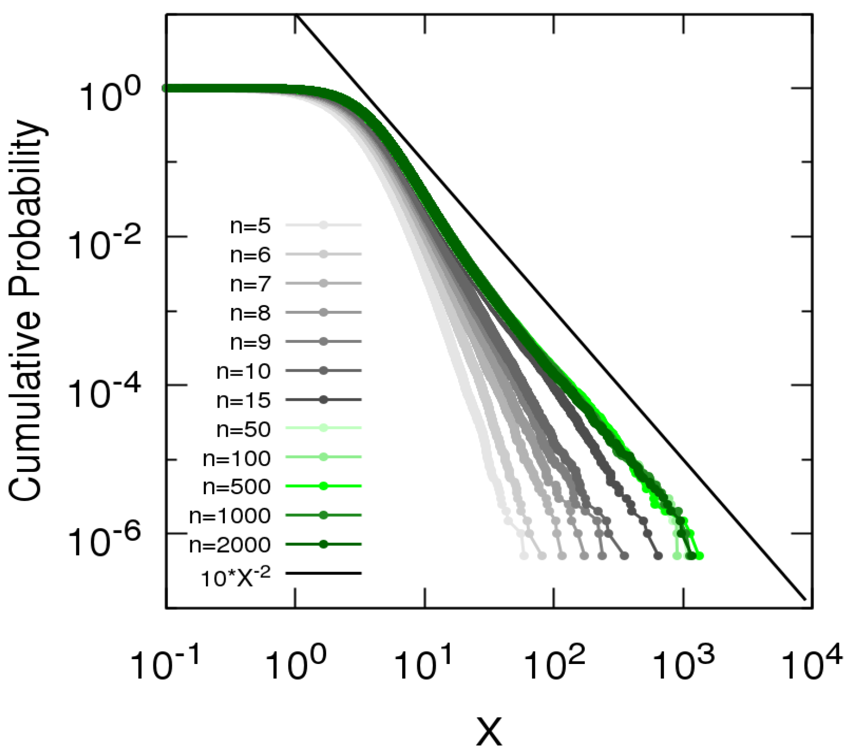
To make manageable the numerical simulations of the model, we cannot keep an endlessly increasing number of entities entering the system and thus we add the rule of removing entities with age greater than n. Figure 1 shows for various values of n in the independent case with half-normally distributed random variables with , for which expression (13) gives . The value is a natural first choice for this parameter since it refers to the standard normal distribution. In this case, one can observe that does not change appreciably for , which suggests that it has converged already for . This means that entities older than 50 time steps have sizes that do not contribute substantially to the sum . In the sequel, we use to be conservative and to obtain reasonable approximations of the asymptotic limit .
Figure 2 presents for the independence (black), Kesten dependence (red) and mixed dependence cases (blue), for (panel a), (panel b) and (panel c). These three values of corresponds, respectively, to , and , as follows from relation (13). Values are chosen in order to analyze the power-law behavior when and , in particular yielding , which corresponds to the Zipf’s law [23]. The tails of are in good visual agreement with these predictions, while the non-asymptotic parts deviate substantially depending on the nature of the dependence. One can observe that the scale factor C, as defined in expression (11), is the smallest for the independence case and the largest for the Kesten dependence. The domain of validity of the power law tail (11) is also the smallest for the independence case and the largest for the Kesten dependence. The distribution for the independence case exhibits the longest intermediate regime before the tail converges to its clean power-law asymptotics. This may be related to the logarithmic correction mentioned above [36].
3.2. Study of the Entities Contributing to the Sum of Sizes
Notwithstanding the similar asymptotic power-law tail behavior (up to a slowly varying function), a closer inspection of the model reveals that the three dependence cases present important and interesting differences in the way the extreme values of X ( or ) are realized. To unveil these differences, we calculate the Herfindahl index, a concentration indicator typically used in finance [37], which is also known as the participation ratio in the physics of spin-glasses [38]. Starting from the size of an individual entity contributing to the sum of sizes, one defines the normalized contribution , which is the fraction of the total system size contributed by entity j. Then, the Herfindahl index reads:
The inverse of the Herfindahl index is a measure of the number of entities that significantly contribute to the sum X of sizes. In particular, it is straightforward to verify that if one entity has size X and all the others have vanishing sizes and that (i.e., equal to the total number of entities in the system) if all entities have identical size equal to . The inverse Herfindahl index thus varies between 1 and t, i.e., from a singular to a full “democratic” contribution to the sum X.
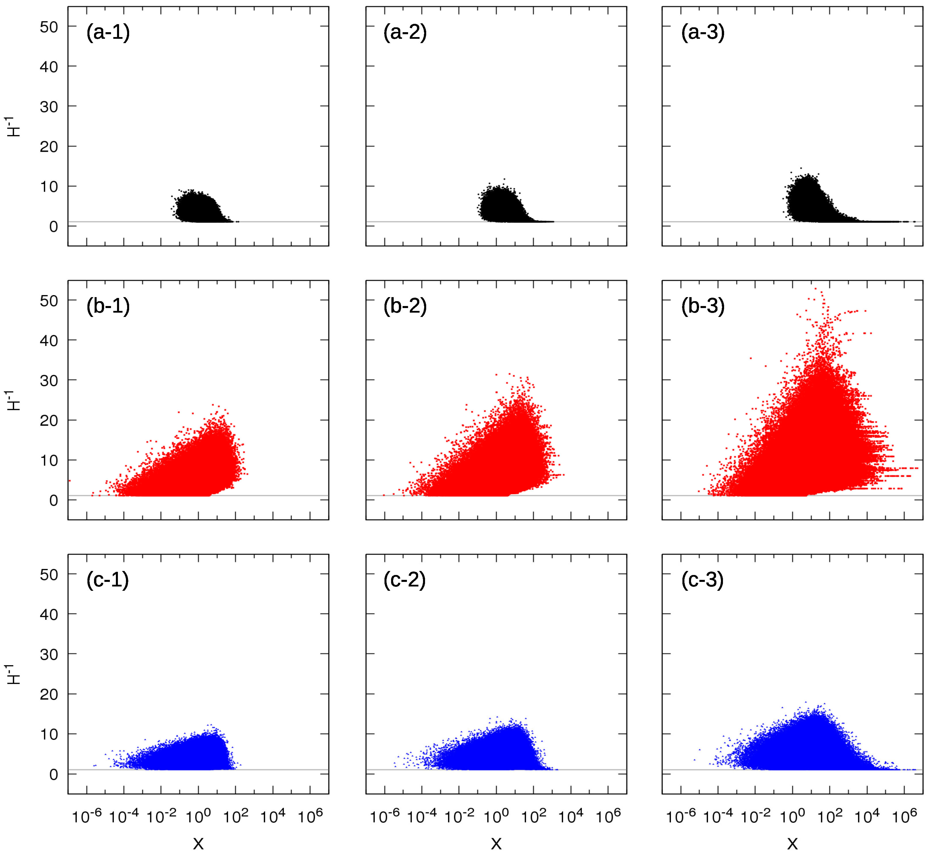
Figure 3 shows scatter plots of as a function of X obtained in the model evolution for all three dependence cases and the three values of used previously. In other words, for each simulation resulting in some , we use the known values of all entity sizes to form the corresponding inverse Herfindahl index. Each row of three panels corresponds to a given dependence model, while each column corresponds to a fixed .
Let us focus first on the second row corresponding to the Kesten dependence case (panels b). The most striking observation is a change of regime. The first regime holds from small to intermediate values of X for which the number of contributing entities can take any value from 1 to a value increasing approximately logarithmically with X. In panel (b-1) for , this regime holds up to . For a larger X, one can observe that the minimum of takes off from the line and there is a minimum strictly larger than 1 necessary to obtain the largest X values. For instance, for the largest sampled values , the number of contributing entities is approximately at least seven. This result has a simple interpretation: due to the dependence between the growth factors across the entities, one very large entity is always surrounded by a “cloud” of similar sized entities. In the single entity dynamical version of the Kesten process, this cloud is made of the cluster of large transient excursions [32].
Let us now turn to the independence case shown in the first row of three panels (panels a). The most striking observation is the progressive shrinkage of the range of values as X gets larger and larger. In addition, there seems to be a rather well-defined threshold such that, for X larger than this threshold, collapses to the single value . In words, the very large values of X that populate the asymptotic power-law behavior of the distribution of X are due to a single entity that overwhelmingly contributes to it. This is reminiscent of a condensation phenomenon, in which a single entity is overwhelmingly larger than all the others, notwithstanding their a priori unlimited number. This might be related to the dragon-king concept [39,40] in an unconventional way: the distribution of the sizes of entities can be seen as the weighted sum of distributions of products of random growth factors. Due to the stationary condition that the random growth factors tend to be smaller than one (the exact technical condition is that the expectation of the logarithm of the random growth factors is negative), only products of random growth factors that have a finite number of terms have a non-negligible size. The system of entities is thus made of a finite (possibly large) number of non-negligible entities at all times. Conditional on the sum X being asymptotically large, the distribution of the entities is non-power-law, but there is a single entity that is of order X, qualifying it as a dragon-king. Interestingly, when sampling over many realizations (statistically or temporally), such set of systems with dragon-kings exhibit in ensemble a pure asymptotic power-law behavior.
Another interesting result when comparing the Kesten and the independence cases is that small values of X, less than the unit size, occur much more frequently in the Kesten case than in the independence case, also a consequence of the strong dependence among entities in the former case: if one entity is small, it is likely that others are small as well.
The mixed dependence (panels c) shows an intermediary behavior between independence and Kesten dependence. In addition, changing the value of the standard deviation of the growth factors does not change the general behavior.
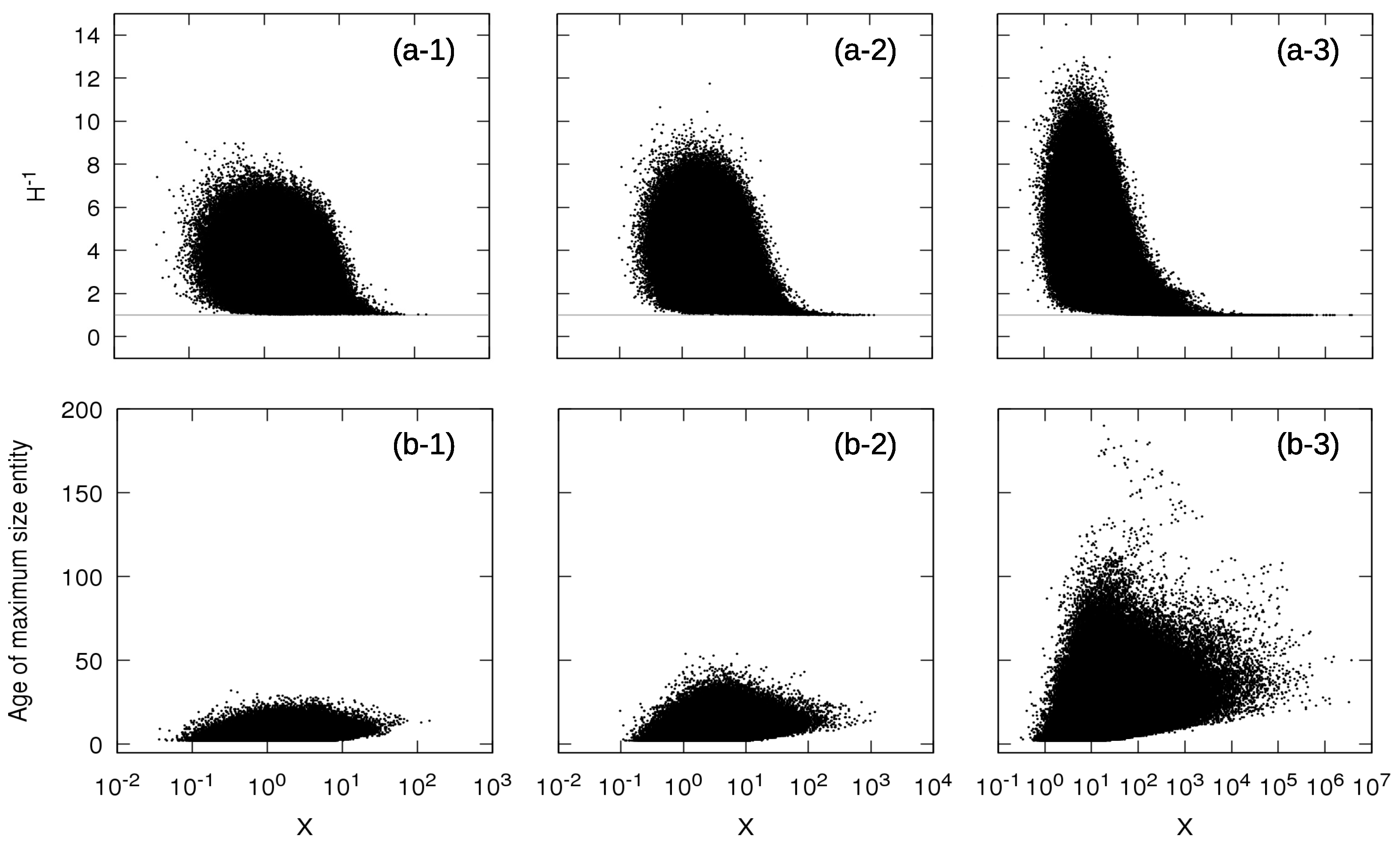
For the independence case, it is interesting to mention that, in addition to the fact that only one entity is responsible for the whole system size X, the age of this maximum size entity is a stochastic variable. This means that the product term that builds the power-law tail of varies as a function of time in its number of multiplicative growth factors, i.e., it does not have the same number of factors at all time steps. Figure 4 shows the age of the entity with maximum size against the total size X of the system for the independence case with (panel b-1), (panel b-2) and (panel b-3): there is a broad distribution of ages of the maximum size entities for large values of X and not a unique age. This observation suggests that the power-law behavior in this case results from the superposition of the statistics of single multiplicative processes at different ages with appropriate statistical weights, as in the superstatistics mechanism mentioned in the introduction [14,15,16]. It is notable that studies following similar ideas with exponential weights established the so-called double Pareto distribution, with power-law tail [41,42].
Finally, numerical simulations in Figure 4 (panels b-1–b-3) suggest that there exist a minimum age for this maximum size entity, which grows approximately logarithmically with X in the asymptotic tail regime. This observation can be rationalized by borrowing the extreme deviation theorem applied to finite products [13]. Parameterizing the probability density function of the independent and identically distributed growth factors as with being a function with a number of “natural” properties such as increasing sufficiently fast as , then the distribution of the product of n independent such variables is given by . In words, the typical tail value of the product of n independent variables is contributed mainly by realizations where all the n random variables are approximately similar in amplitude and equal to , so that their product (with n term) recover . The term n in front of in the exponential correspond to taking the product of n probability density functions of the independent growth factors . Fixing to a large value X, the value that maximizes is given by:
and denotes the derivative of . Searching for a solution of the form , where c is a constant, we find that c solves the equation . Thus, for the process (7), for a given large X, the product term that contributes the most to a given large Sigma-Pi X contains at least factors. This means that a large X is minimally controlled by the term with about factors , i.e., with an age . This result is essentially independent of the specific form of the probability density function of the growth factors , as long as obeys the conditions for the validity of the extreme deviation theorem.
4. Conclusions
Two main conclusions can be drawn from this work. First, for sums of products of random growth factors, referred above as Sigma-Pi structures, the dependence among the product terms (the “entities”) that may result from some dependence between the growth factors do not impact the asymptotic power-law of the distribution of these Sigma-Pi variables, up to slowly varying functions. Simulations of our simple growth model with distinct dependence types together with previous theoretical studies on the Kesten process and of the sum of products of independent random variable support this conclusion. Indeed, the essential ingredient for the asymptotic power-law tail seems to be the Sigma-Pi structure, regardless of the dependence type. This conjecture is still to be formally proved.
Second, although the exponent of the asymptotic power-law tail is not influenced by the dependence type among entities, the nature of the construction of the events populating the tail differs in each dependence case. In the independence case, only one entity in the sum contributes to it asymptotically. In contrast, in the Kesten dependence case, as a result of the strong dependence between the growth factors across entities, several entities contribute to the sum asymptotically. These insights are important in the modeling of real physical, biological or economic systems, complementing the ubiquitous power-law tail behavior with additional information on the internal structure of the system.
Acknowledgments
The author Arthur Matsuo Yamashita Rios de Sousa acknowledges funding from the Monbukagakusho MEXT Scholarship (Japanese Ministry of Education, Culture, Sports, Science and Technology).
Author Contributions
All authors contributed equally to this work.
Conflicts of Interest
The authors declare no conflict of interest.
Appendix A
We use a heuristic derivation of the power-law tail of Sigma-Pi structures, using the method of moments. This is offered as a support of the conjecture that the probability distribution function of a Sigma-Pi X presents power-law tail behavior with the same exponent for any dependence type across terms in the sum, when all growth factors within each product term are independent.
Consider the general Sigma-Pi with arbitrary coefficients :
where are identically distributed random variables with probability distribution function . Let us assume that such that . Among the random factors , let us denote as the number of independent random variables . Then, the moment of order of is given by:
The multinomial expansion [43] suggests the following representation:
where includes the other terms of the expansion involving crossed products. Using this representation and considering the restricted cases where all variables in a product term are independent, we arrive at:
where corresponds to the integration of over the s independent variables on the right side of expression (A2). The function carries the information on the dependence between the growth factors .
We assume that the coefficients can be parameterized as:
for some function h. Then, letting , the sum term on the right side of (A4) is the Maclaurin series of the function (excluding the first term ), which leads to:
For the growth model in this paper, . Thus, the function h is:
provided that .
Suppose that such that . Expanding around , we have:
Then, around , but keeping (moment finite but close to the divergence point):
Identifying the real moment of order of the random variable X as the Mellin transform M of its probability density function , a pole in the Mellin transform of a function corresponds to a power law tail. Thus, applying the inverse Melling transform to (A9) yields the power-law behavior [44,45]:
where H is the Heaviside step function.
A comparison with the exact mathematical derivations [27] for the Kesten process and [36] for the independent case indicates that the non-diagonal term does not alter the power-law behavior predicted by only taking into account the diagonal term, i.e., the first term on the right side of expression (A3). We conjecture that this still holds for a large class of dependence types between the stochastic growth factors .
Appendix B
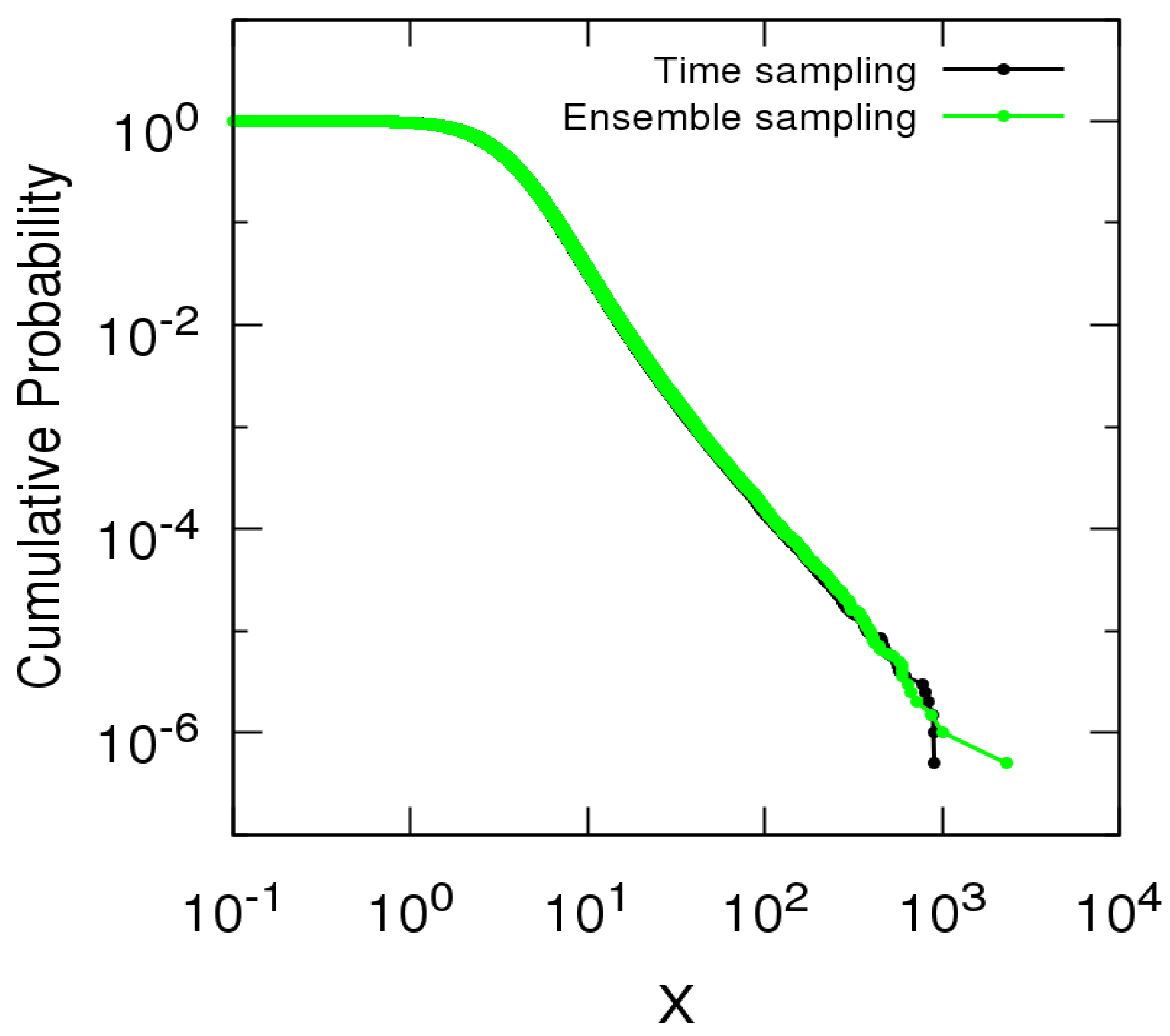
We compare the complementary cumulative distribution function of the sum X of entity sizes for the independence case with computed over time during the evolution of the model removing entities older than and the one computed using a statistical ensemble of entities with increasing distinct ages ranging from 1 to 100.
Figure A1 shows a good agreement between the distribution function using time sampling (black) and ensemble sampling (green), which provides evidence of the ergodicity of the process. Similar results were found for the Kesten and mixed dependence cases and for different values of .
Figure A1.
Complementary cumulative distribution function of the sum X of entity sizes for the independence case with using time sampling (black) and ensemble sampling (green).
Figure A1.
Complementary cumulative distribution function of the sum X of entity sizes for the independence case with using time sampling (black) and ensemble sampling (green).
References
- Clauset, A.; Shalizi, C.R.; Newman, M.E. Power-law distributions in empirical data. SIAM Rev. 2009, 51, 661–703. [Google Scholar] [CrossRef]
- Mitchell, M. Complexity: A Guided Tour; Oxford University Press: New York, NY, USA, 2009. [Google Scholar]
- Newman, M.E. Power laws, Pareto distributions and Zipf’s law. Contemp. Phys. 2005, 46, 323–351. [Google Scholar] [CrossRef]
- Foss, S.; Korshunov, D.; Zachary, S. An Introduction to Heavy-Tailed and Subexponential Distributions; Springer: New York, NY, USA, 2011; Volume 6. [Google Scholar]
- Mitzenmacher, M. A brief history of generative models for power law and lognormal distributions. Internet Math. 2004, 1, 226–251. [Google Scholar] [CrossRef]
- Sornette, D. Critical Phenomena in Natural Sciences; Springer: Berlin/Heidelberg, Germany, 2006. [Google Scholar]
- Yule, G.U. A mathematical theory of evolution, based on the conclusions of Dr. JC Willis, FRS. Philos. Trans. R. Soc. Lond. Ser. B Contain. Pap. Biol. Character 1925, 213, 21–87. [Google Scholar] [CrossRef]
- Simon, H.A. On a class of skew distribution functions. Biometrika 1955, 42, 425–440. [Google Scholar] [CrossRef]
- Barabási, A.L.; Albert, R.; Jeong, H. Mean-field theory for scale-free random networks. Phys. A Stat. Mech. Appl. 1999, 272, 173–187. [Google Scholar] [CrossRef]
- Bak, P.; Tang, C.; Wiesenfeld, K. Self-organized criticality: An explanation of the 1/f noise. Phys. Rev. Lett. 1987, 59, 381. [Google Scholar] [CrossRef] [PubMed]
- Bak, P. How Nature Works: The Science of Self-Organized Criticality; Copernicus Press: New York, NY, USA, 1996. [Google Scholar]
- Taguchi, Y.H.; Takayasu, H. Power law velocity fluctuations due to inelastic collisions in numerically simulated vibrated bed of powder. Europhys. Lett. 1995, 30, 499. [Google Scholar] [CrossRef]
- Frisch, U.; Sornette, D. Extreme deviations and applications. J. Phys. I 1997, 7, 1155–1171. [Google Scholar] [CrossRef]
- Beck, C.; Cohen, E.G.D. Superstatistics. Phys. A Stat. Mech. Appl. 2003, 322, 267–275. [Google Scholar] [CrossRef]
- Beck, C. Superstatistics: Theoretical concepts and physical applications. arXiv, 2007; arXiv:0705.3832. [Google Scholar]
- Hanel, R.; Thurner, S.; Gell-Mann, M. Generalized entropies and the transformation group of superstatistics. Proc. Natl. Acad. Sci. USA 2011, 108, 6390–6394. [Google Scholar] [CrossRef]
- Tsallis, C. Possible generalization of Boltzmann-Gibbs statistics. J. Stat. Phys. 1988, 52, 479–487. [Google Scholar] [CrossRef]
- Amaral, L.A.N.; Buldyrev, S.V.; Havlin, S.; Salinger, M.A.; Stanley, H.E. Power law scaling for a system of interacting units with complex internal structure. Phys. Rev. Lett. 1998, 80, 1385. [Google Scholar] [CrossRef]
- Huynen, M.A.; van Nimwegen, E. The frequency distribution of gene family sizes in complete genomes. Mol. Biol. Evol. 1998, 15, 583–589. [Google Scholar] [CrossRef] [PubMed]
- Blank, A.; Solomon, S. Power laws in cities population, financial markets and internet sites (scaling in systems with a variable number of components). Phys. A Stat. Mech. Appl. 2000, 287, 279–288. [Google Scholar] [CrossRef]
- Keitt, T.H.; Amaral, L.A.; Buldyrev, S.V.; Stanley, H.E. Scaling in the growth of geographically subdivided populations: Invariant patterns from a continent-wide biological survey. Philos. Trans. R. Soc. Lond. B Biol. Sci. 2002, 357, 627–633. [Google Scholar] [CrossRef] [PubMed]
- Picoli, S., Jr.; Mendes, R.S. Universal features in the growth dynamics of religious activities. Phys. Rev. E 2008, 77, 036105. [Google Scholar] [CrossRef] [PubMed]
- Saichev, A.I.; Malevergne, Y.; Sornette, D. Theory of Zipf’s Law and Beyond; Springer: Berlin/Heidelberg, Germany, 2009; Volume 632. [Google Scholar]
- Alves, L.G.; Ribeiro, H.V.; Mendes, R.S. Scaling laws in the dynamics of crime growth rate. Phys. A Stat. Mech. Appl. 2013, 392, 2672–2679. [Google Scholar] [CrossRef]
- Takayasu, M.; Watanabe, H.; Takayasu, H. Generalised central limit theorems for growth rate distribution of complex systems. J. Stat. Phys. 2014, 155, 47–71. [Google Scholar] [CrossRef]
- Sutton, J. Gibrat’s legacy. J. Econ. Lit. 1997, 35, 40–59. [Google Scholar]
- Kesten, H. Random difference equations and renewal theory for products of random matrices. Acta Math. 1973, 131, 207–248. [Google Scholar] [CrossRef]
- Goldie, C.M. Implicit renewal theory and tails of solutions of random equations. Ann. Appl. Probab. 1991, 126–166. [Google Scholar] [CrossRef]
- Takayasu, H.; Sato, A.H.; Takayasu, M. Stable infinite variance fluctuations in randomly amplified Langevin systems. Phys. Rev. Lett. 1997, 79, 966. [Google Scholar] [CrossRef]
- Sornette, D. Multiplicative processes and power laws. Phys. Rev. E 1998, 57, 4811. [Google Scholar] [CrossRef]
- Buraczewski, D.; Damek, E.; Mikosch, T. Stochastic Models with Power-Law Tails; Springer: New York, NY, USA, 2016. [Google Scholar]
- Sornette, D.; Cont, R. Convergent multiplicative processes repelled from zero: Power laws and truncated power laws. J. Phys. I 1997, 7, 431–444. [Google Scholar] [CrossRef]
- Hisano, R.; Sornette, D.; Mizuno, T. Predicted and verified deviations from Zipf’s law in ecology of competing products. Phys. Rev. E 2011, 84, 026117. [Google Scholar] [CrossRef] [PubMed]
- Malevergne, Y.; Saichev, A.; Sornette, D. Zipf’s law and maximum sustainable growth. J. Econ. Dyn. Control 2013, 37, 1195–1212. [Google Scholar] [CrossRef]
- Weisstein, E.W. Half-Normal Distribution. From MathWorld—A Wolfram Web Resource. Available online: http://mathworld.wolfram.com/Half-NormalDistribution.html (accessed on 16 August 2017).
- Mikosch, T.; Rezapour, M.; Wintenberger, O. Heavy tails for an alternative stochastic perpetuity model. arXiv, 2017; arXiv:1703.07272. [Google Scholar]
- Herfindahl-Hirschman Index—HHI. Available online: http://investopedia.com/terms/h/hhi.asp (accessed on 20 July 2017).
- Mézard, M.; Parisi, G.; Virasoro, M.A. Random free energies in spin glasses. J. Phys. Lett. 1985, 46, 217–222. [Google Scholar] [CrossRef]
- Sornette, D. Dragon-kings, black swans and the prediction of crises. Int. J. Terrasp. Sci. Eng. 2009, 2, 1–18. [Google Scholar] [CrossRef]
- Sornette, D.; Ouillon, G. Dragon-kings: Mechanisms, statistical methods and empirical evidence. Eur. Phys. J. Spec. Top. 2012, 205, 1–26. [Google Scholar] [CrossRef]
- Huberman, B.A.; Adamic, L.A. Internet: Growth dynamics of the world-wide web. Nature 1999, 401, 131. [Google Scholar]
- Reed, W.J. The Pareto law of incomes—An explanation and an extension. Phys. A Stat. Mech. Appl. 2003, 319, 469–486. [Google Scholar] [CrossRef]
- Weisstein, E.W. Multinomial Series. From MathWorld—A Wolfram Web Resource. Available online: http://mathworld.wolfram.com/MultinomialSeries.html (accessed on 16 August 2017).
- Flajolet, P.; Gourdon, X.; Dumas, P. Mellin transforms and asymptotics: Harmonic sums. Theor. Comput. Sci. 1995, 144, 3–58. [Google Scholar] [CrossRef]
- Weisstein, E.W. Mellin Transform. From MathWorld—A Wolfram Web Resource. Available online: http://mathworld.wolfram.com/MellinTransform.html (accessed on 16 August 2017).
Figure 1.
Complementary cumulative distribution function of (7) or equivalently (10) for the independence case with half-normally distributed random variables with , corresponding to , for and 2000.

Figure 2.
Numerical construction of the complementary cumulative distribution function of the random variable (7) or equivalently (10) in the limit of large t or n, for independence (black), Kesten dependence (red) and mixed dependence cases (blue) with (a) ; (b) and (c) . Following expression (13), the tails are consistent with the expected values of the exponents , and , respectively, regardless of the dependence type, as shown by the straight grey lines.
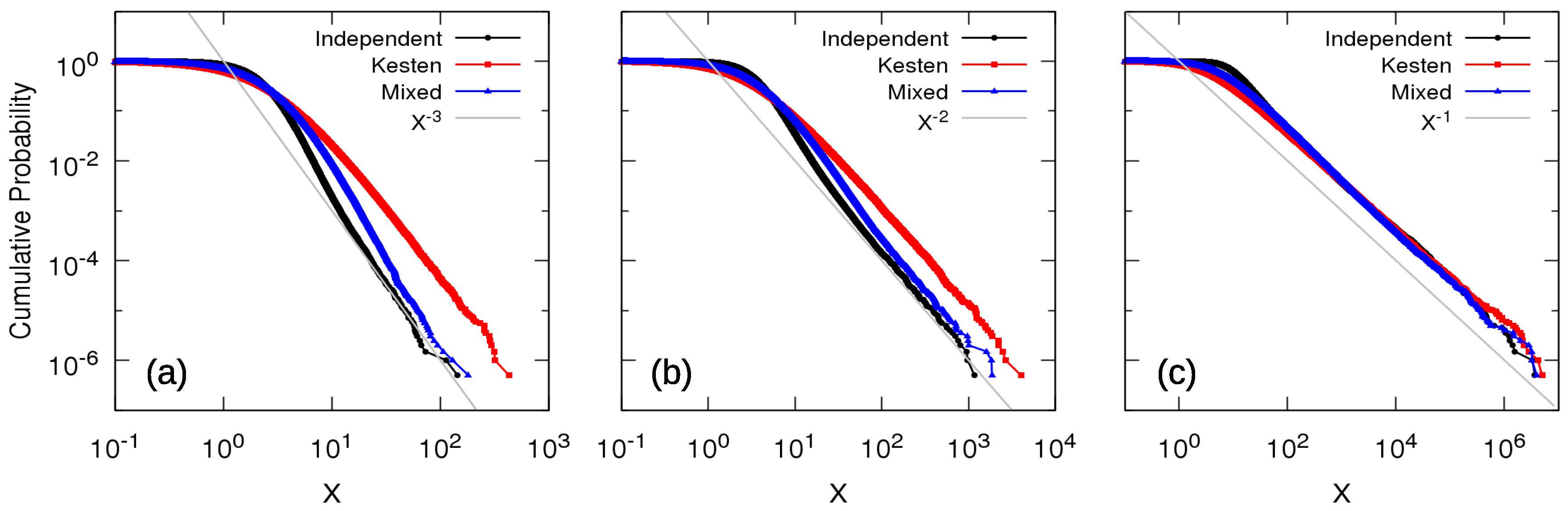
Figure 3.
Relationship between the inverse Herfindahl index and the sum X of sizes where the three rows correspond to the three cases of dependence and the three columns correspond to three different values of : (a-1) independence with ; (a-2) independence with ; (a-3) independence with ; (b-1) Kesten dependence with ; (b-2) Kesten dependence with ; (b-3) Kesten dependence with ; (c-1) mixed dependence with ; (c-2) mixed dependence with and (c-3) mixed dependence with . The horizontal grey lines indicate . Focusing on large values of X, corresponding to the power-law tail of the distribution function , only one entity contributes to the total size of the system in the independence case, but, in the Kesten dependence case, the total size is always due to the contribution of several entities (see text).

Figure 4.
(a) relationship between the inverse of the Herfindahl index and the sum X of sizes and (b) relationship between the inverse of the age of the maximum size entity and the sum X of sizes for the independence case with: (a-1,b-1) ; (a-2,b-2) and (a-3,b-3) . The horizontal gray lines indicate . For the independence case, large values of X, corresponding to the power-law tail of the distribution function , are made of a single entity, but its age is a stochastic variable changing with time and with realizations.
© 2017 by the authors. Licensee MDPI, Basel, Switzerland. This article is an open access article distributed under the terms and conditions of the Creative Commons Attribution (CC BY) license (http://creativecommons.org/licenses/by/4.0/).
Share and Cite
MDPI and ACS Style
Sousa, A.M.Y.R.d.; Takayasu, H.; Sornette, D.; Takayasu, M. Power-Law Distributions from Sigma-Pi Structure of Sums of Random Multiplicative Processes. Entropy 2017, 19, 417. https://doi.org/10.3390/e19080417
AMA Style
Sousa AMYRd, Takayasu H, Sornette D, Takayasu M. Power-Law Distributions from Sigma-Pi Structure of Sums of Random Multiplicative Processes. Entropy. 2017; 19(8):417. https://doi.org/10.3390/e19080417
Chicago/Turabian StyleSousa, Arthur Matsuo Yamashita Rios de, Hideki Takayasu, Didier Sornette, and Misako Takayasu. 2017. "Power-Law Distributions from Sigma-Pi Structure of Sums of Random Multiplicative Processes" Entropy 19, no. 8: 417. https://doi.org/10.3390/e19080417
Note that from the first issue of 2016, this journal uses article numbers instead of page numbers. See further details here.