Survey on Probabilistic Models of Low-Rank Matrix Factorizations


1
School of Science, Xi’an University of Architecture and Technology, Xi’an 710055, China
2
School of Architecture, Xi’an University of Architecture and Technology, Xi’an 710055, China
*
Author to whom correspondence should be addressed.
Entropy 2017, 19(8), 424; https://doi.org/10.3390/e19080424
Submission received: 12 June 2017
/
Revised: 11 August 2017
/
Accepted: 16 August 2017
/
Published: 19 August 2017
(This article belongs to the Special Issue Information Theory in Machine Learning and Data Science)
Abstract
:Low-rank matrix factorizations such as Principal Component Analysis (PCA), Singular Value Decomposition (SVD) and Non-negative Matrix Factorization (NMF) are a large class of methods for pursuing the low-rank approximation of a given data matrix. The conventional factorization models are based on the assumption that the data matrices are contaminated stochastically by some type of noise. Thus the point estimations of low-rank components can be obtained by Maximum Likelihood (ML) estimation or Maximum a posteriori (MAP). In the past decade, a variety of probabilistic models of low-rank matrix factorizations have emerged. The most significant difference between low-rank matrix factorizations and their corresponding probabilistic models is that the latter treat the low-rank components as random variables. This paper makes a survey of the probabilistic models of low-rank matrix factorizations. Firstly, we review some probability distributions commonly-used in probabilistic models of low-rank matrix factorizations and introduce the conjugate priors of some probability distributions to simplify the Bayesian inference. Then we provide two main inference methods for probabilistic low-rank matrix factorizations, i.e., Gibbs sampling and variational Bayesian inference. Next, we classify roughly the important probabilistic models of low-rank matrix factorizations into several categories and review them respectively. The categories are performed via different matrix factorizations formulations, which mainly include PCA, matrix factorizations, robust PCA, NMF and tensor factorizations. Finally, we discuss the research issues needed to be studied in the future.
1. Introduction
In many practical applications, a commonly-used assumption is that the dataset approximately lies in a low-dimensional linear subspace. Low-rank matrix factorizations (or decompositions, the two terms are used interchangeably) are just a type of method for recovering the low-rank structure, removing noise and completing missing values. Principal Component Analysis (PCA) [1], a traditional matrix factorization method, copes effectively with the situation that the dataset is contaminated by Gaussian noise. If the mean vector is set to be a zero vector, then PCA is transformed into Singular Value Decomposition (SVD) [2]. Classical PCA approximates the low-rank representation according to eigen decomposition of the covariance matrix of a dataset to be investigated. When there are outliers or large sparse errors, the original version of PCA does not work well for obtaining the low-rank representations. In this case, many robust methods of PCA have been extensively studied such as L1-PCA [3], L1-norm maximization PCA [4], L21-norm maximization PCA [5] and so on.
In this paper, low-rank matrix factorizations refer to a general formulation of matrix factorizations and they mainly consist of PCA, matrix factorizations, robust PCA [6], Non-negative Matrix Factorization (NMF) [7] and tensor decompositions [8]. As a matter of fact, matrix factorizations are usually a special case of PCA and they directly factorize a data matrix into the product of two low-rank matrices without consideration of the mean vector. Matrix completion aims to complete all missing values according to the approximate low-rank structure and it is mathematically described as a nuclear norm minimization problem [9]. To this end, we regard matrix completion as a special case of matrix factorizations. In addition, robust PCA decomposes the data matrix into the superposition of a low-rank matrix and a sparse component, and recovers both the low-rank and the sparse matrices via principal component pursuit [6].
Low-rank matrix factorizations suppose that the low-rank components are corrupted by certain random noise and the low-rank matrices are deterministic unknown parameters. Maximum Likelihood (ML) estimation and Maximum a posteriori (MAP) are two most popular methodologies used in estimating the low-rank matrices. A prominent advantage of the aforementioned point estimate methods is that they are simple and easy to implement. However, we can not obtain the probability distributions of the low-rank matrices that are pre-requisite in exploring the generative models. Probabilistic models of low-rank matrix factorizations can approximate the true probability distributions of the low-rank matrices and they have attracted a great deal of attention in the past two decades. These models have been widely applied in the fields of signal and image processing, computer vision, machine learning and so on.
Tipping and Bishop [10] originally presented probabilistic PCA in which the latent variables are assumed to be a unit isotropic Gaussian distribution. Subsequently, several other probabilistic models of PCA were proposed successively, such as Bayesian PCA [11], Robust L1 PCA [12], Bayesian robust PCA [13] and so on. As a special case of probabilistic models of PCA, Bayesian matrix factorization [14] placed zero-mean spherical Gaussian priors on two low-rank matrices and it was applied to collaborative filtering. Probabilistic models of matrix factorizations also include probabilistic matrix factorization [15], Bayesian probabilistic matrix factorization [16], robust Bayesian matrix factorization [17], probabilistic robust matrix factorization [18], sparse Bayesian matrix completion [19], Bayesian robust matrix factorization [20] and Bayesian L1-norm low-rank matrix factorizations [21].
As to robust PCA, we take the small dense noise into account. In other words, the data matrix is decomposed into the sum of a low-rank matrix, a sparse noise matrix and a dense Gaussian noise matrix. Hence, the corresponding probabilistic models are robust to outliers and large sparse noise, and they are mainly composed of Bayesian robust PCA [22], variational Bayesian robust PCA [23] and sparse Bayesian robust PCA [19]. As another type of low-rank matrix factorizations, NMF decomposes a non-negative data matrix into the product of two non-negative low-rank matrices. Compared with PCA, NMF is a technique which learns holistic, not parts-based representations [7]. Different probabilistic models of NMF were proposed in [24,25,26,27,28]. Recently, probabilistic models of low-rank matrix factorizations are also extended to the case of tensor decompositions. Tucker decomposition and CANDECOMP/PARAFAC (CP) decomposition are two most important tensor decompositions. By generalizing the subspace approximation, some new low rank tensor decompositions have emerged, such as the hierarchical Tucker (HT) format [29,30], the tensor tree structure [31] and the tensor train (TT) format [32]. Among them, the TT format is a special case of the HT and the tensor tree structure [33]. The probabilistic models of the Tucker were presented in [34,35,36] and that of the CP were developed in [37,38,39,40,41,42,43,44,45,46,47,48].
For probabilistic models of low-rank matrix factorizations, there are three most frequently used statistical approaches for inferring the corresponding probability distributions or parameters, i.e., Expectation Maximization (EM) [49,50,51,52,53,54], Gibbs sampling(or a Gibbs sampler) [54,55,56,57,58,59,60,61,62] and variational Bayesian (VB) inference [54,62,63,64,65,66,67,68,69,70,71]. EM is an iterative algorithm with guaranteed the local convergence for ML estimation and does not require explicit evaluation of the likelihood function [70]. Although it has many advantages over ML, EM tends to be limited in applications because of its serious requirements for the posterior of the hidden variables and can not be used to solve complex Bayesian models [70]. However, VB inference relaxes some limitations of the EM algorithm and ameliorates its shortcomings. As a means of VB, Gibbs sampling is another method used to infer the probability distributions of all parameters and hidden variables.
This paper provides a survey on probabilistic models of low-rank matrix factorizations. Firstly, we review the significant probability distributions commonly-used in probabilistic low-rank matrix factorizations and introduce the conjugate priors that are essential to Bayesian statistics. Then we present two most important methods for inferring the probability distributions, that is, Gibbs sampling and VB inference. Next, we roughly divide the available low-rank matrix factorization models into five categories: PCA, matrix factorizations, robust PCA, NMF and tensor decompositions. For each category, we provide a detailed overview of the corresponding probabilistic models.
A central task for probabilistic low-rank matrix factorizations is to predict the missing or incomplete data. For the sake of concise descriptions, we do not consider the missing entries in all models except the sparse Bayesian model of matrix completion. The remainder of this paper is listed as below. Section 2 introduces the commonly-used probability distributions and the conjugate priors. Section 3 presents two frequently used inferring methods: Gibbs sampling and VB inference. Probabilistic models of PCA and matrix factorizations are reviewed respectively in Section 4 and Section 5. Section 6 and Section 7 survey probabilistic models of robust PCA and NMF, respectively. Section 8 provides other probabilistic models of low-rank matrix factorizations and probabilistic tensor factorizations. The conclusions and future research directions are drawn in Section 9.
Notation: Let be the set of real numbers and the set of non-negative real numbers. We denote scalars with italic letters (e.g., ), vectors with bold letters (e.g., ), matrices with bold capital letters (e.g., ) and sets with italic capital letters (e.g., ). Given a matrix , its ith row, jth column and (i, j)th element are expressed as , and , respectively. If is square, let and be the trace and the determinant of , respectively.
2. Probability Distributions and Conjugate Priors
This section will introduce some probability distributions commonly adopted in probabilistic models of low-rank matrix factorizations and discuss the conjugate priors for algebraic and intuitive convenience in Bayesian statistics.
2.1. Probability Distributions
We consider some significant probability distributions that will be needed in the following sections. Given a univariate random variable or a random vector , we denote its probability density/mass function by or . Let be the expectation of and the covariance matrix of .
Several probability distributions such as Gamma distribution and Beta distribution deal with the gamma function defined by
We summarize the probability distributions used frequently in probabilistic models of low-rank matrix factorizations, as shown in Table 1. In this table, we list the notation for each probability distribution, the probability density/mass function, the expectation and the variance/covariance respectively. For the Wishart distribution , the term is given by
where the positive integer is named the degrees of freedom. For the generalized inverse Gaussian distribution , is a modified Bessel function of the second kind. For brevity of notation, we stipulate a few simple representations of a random variable or vector. For instance, if follows a multivariate Gaussian distribution with mean and covariance matrix , we can write this distribution as , or , or . In addition, some probability distributions can be extended to the multivariate case under identical conditions. The following cites an example: if random variables and are independent, then we have with the probability density function , where and .
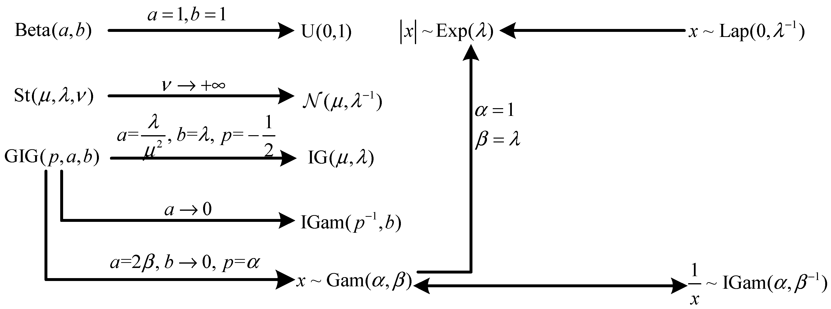
There exist close relationships among probability distributions listed in Table 1, as shown partially in Figure 1. Refer to [54,62,66] for more probability distributions. Moreover, some continuous random variables can be reformulated as Gaussian scale mixtures with other distributions from a hierarchical viewpoint. Now, we give two most frequently used examples as below.
Example 1.
For given parameter , if the conditional probability distribution of is and the prior distribution of is , then we have .
The probability density function of is derived as:
Meanwhile, it holds that
where is the Laplace transform and is the inverse Laplace transform. Hence, we get .
Example 2.
For given parameters and , if the conditional probability distribution of is and the prior distribution of is , then it holds that , where is a fixed parameter.
The derivation process for is described as follows:
So, .
2.2. Conjugate Priors
Let be a random vector with the parameter vector and a collection of N observed samples. In the presence of latent variables, they are also absorbed into . For given , the conditional probability density/mass function of is denoted by . Thus, we can construct the likelihood function:
As for variational Bayesian methods, the parameter vector is usually assumed to be stochastic. Here, the prior distribution of is expressed as .
To simplify Bayesian analysis, we hope that the posterior distribution is in the same functional form as the prior . Under this circumstance, the prior and the posterior are called conjugate distributions and the prior is also called a conjugate prior for the likelihood function [54,66]. In the following, we provide three most commonly-used examples of conjugate priors.
Example 3.
Assume that random variable obeys the Bernoulli distribution with parameter . We have the likelihood function for :
where the observations . In consideration of the form of , we stipulate the prior distribution of as the Beta distribution with parameters and :
At this moment, we get the posterior distribution of via the Bayes’ rule:
Because
we have . The conclusion means that the Beta distribution is the conjugate prior for the Bernoulli likelihood.
Example 4.
Assume that random variable obeys a univariate Gaussian distribution , where is also named the precision. The likelihood function of for given is
We further suppose that the prior distribution of is the Gamma distribution with parameters a and b. Let be the posterior distribution of . Then we have
Because
we get . Therefore, the conjugate prior of the precision for a Gaussian likelihood is a Gamma distribution.
Example 5.
Assume that random vector obeys a d-dimensional Gaussian distribution , where , the inverse of covariance matrix, is called the precision matrix. We consider the case that both and are unknown. Thus, the likelihood function for is
The prior distribution of is given by a Gaussian–Wishart distribution with the joint probability density function:
where and are the fixed hyperparameters. Hence, it holds that
Denote and . To obtain the above probability density function, we first derive the following formula:
Then we get
Because , we have
This example shows that the conjugate prior of for a multivariate Gaussian is a Gaussian–Wishart distribution.
There are some other conclusions on the conjugate priors. For instance, given Gaussian likelihood, the conjugate prior for the mean is another Gaussian distribution, the conjugate prior for the precision matrix is a Wishart distribution. All probability distributions discussed in Section 2.1 belong to a broad class of distributions, that is, the exponential family. It is shown that the exponential family distributions have conjugate priors [54,66,72].
3. Gibbs Sampling and Variational Bayesian Inference
Due to the existence of the latent variables or unknown parameters, computing the posterior distribution is analytically intractable in general. In this section, we will provide two approximation inference methods: Gibbs sampling and variational Bayesian inference.
3.1. Gibbs Sampling
As a powerful framework for sampling from a probability distribution, Markov chain Monte Carlo (MCMC) methods, also called Markov chain simulation, construct a Markov chain such that its equilibrium distribution is the desired distribution [73,74,75,76,77,78,79,80]. Random walk Monte Carlo methods are a large subclass of MCMC and they include mainly Metropolis–Hastings [54,62,66,81], Gibbs sampling, Slice sampling [54,62,66], Multiple-try Metropolis [82,83].
Gibbs sampling or Gibbs sampler, a simple MCMC algorithm, is especially applicable for approximating a sequence of observations by a specified probability distribution when direct sampling is intractable. In addition, the basic version of Gibbs sampling is also a special case of the Metropolis–Hastings algorithm [54,62]. In detailed implementation, Gibbs sampling adopts the strategy of sampling from a conditional probability distribution instead of marginalizing the joint probability distribution by integrating over other variables. In other words, Gibbs sampling generates alternatively an instance from its corresponding conditional probability distribution by fixing other variables.
Let be M blocks of random variables and set . The joint probability distribution of is written as . In this subsection, we only consider the case that it is difficult to directly sampling from the joint probability distribution . To this end, we can sample each component from marginal distribution in order. The marginal distribution of can be theoretically obtained by the following formulation:
Generally speaking, the integrating term in the above formula is not tractable. A wise sampling strategy is that we generate according to the conditional probability distribution , where . By using Bayes’ rule, the relationship between the conditional probability distribution and the joint probability distribution is given as follows:
The sampling procedure is repeated by cycling through all variables. We summarize the outline of Gibbs sampling as below.
| 1. Initialize . |
| 2. For |
| For |
| Generate from the conditional probability distribution . |
| End |
| End |
In the above sampling procedure, T is the maximum number of iterations. Therefore, we have T samples . To alleviate the influence of random initializations, we can ignore the samples within the burn-in period. Although Gibbs sampling is commonly efficient in obtaining marginal distributions from conditional distributions, it can be highly inefficient for some cases such as sampling from Mexican hat like distribution [53].
The Metropolis algorithm is an instance of MCMC algorithms and walks randomly with an acceptance/rejection rule until the convergence is achieved. As the generalization of Metropolis algorithm, the Metropolis–Hastings algorithm modifies the jumping rules and its convergence speed is improved [66]. Broadly speaking, the advanced Gibbs sampling algorithm can be regarded as a special case of the Metropolis–Hastings algorithm. The Gibbs sampler is applicable for models that are conditionally conjugate, while the Metropolis algorithm can be used for not conditionally conjugate models. Hence, we can combine both the Gibbs sampler and the Metropolis algorithm to sample from complex distributions [66].
3.2. Variational Bayesian Inference
Another widely used class of approximating the marginal probability distribution is the variational Bayesian (VB) inference [54]. We still use the notation to represent a matrix composed of observed datum and to represent a vector constructed by blocks of latent variables. In VB methods, both and are assumed to be stochastic.
Given the prior distribution and the data likelihood , the probability distribution of data matrix , also called the evidence, can be calculated as . Then we derive the conditional probability distribution of via Bayes’ rule:
However, the integrating term is analytically intractable under normal conditions. Now, we harness VB methods to approximate the posterior distribution as well as .
Let be the trial probability distribution of . The log of the probability distribution is decomposed as below:
where and . The term is called the Kullback–Leibler (KL) divergence [54,84,85,86,87] between and , and is the lower bound of that achieves its lower bound if and only if (or equivalently ). The above divergence can also be explained as the information gain changing from the prior to the posterior [85].
Another perspective for Equation (23) is that,
The above inequality is obtained by Jensen’s inequality. The negative lower bound is called the free energy [88,89].
The KL divergence can be regarded as a metric for evaluating the approximation performance of the prior distribution over the posterior distribution [54]. In the light of Equation (23), minimizing is equivalent to maximizing . What’s more, the lower bound can be further derived as below:
The above Equation means that can also be regarded as the expectation of the log likelihood function with respect to .
To reduce the difficulty of approximating the trial distribution , we partition all latent variables into M disjoint block variables and assume that are mutually independent. Based on the above assumption, we have
Afterwards, we utilize the mean field theory to obtain the approximation of . Concretely speaking, we update each in turn. Let be unknown and be fixed. Under this circumstance, we can get the optimal by solving the following variational maximization problem:
Plugging Equation (26) into the lower bound of , we have
where “const” is a term independent of and is a new probability distribution whose log is defined by
Therefore, is the optimal solution of problem (27) obtained by minimizing the KL divergence between and .
An advantage of the VB methods is that they are immune to over fitting. But they also have some shortcomings. For example, the probability distributions derived via VB have always less probability mass in the wings than the true solution and this systematic bias may break applications. A VB method approximates a full posterior distribution by maximizing the corresponding lower bound on the marginal likelihood and it can only handle a smaller dataset. In contrast, the stochastic variational inference optimizes a subset at each iteration. This batch inference algorithm is scalable and outperforms traditional variational inference methods [90,91].
3.3. Comparisons between Gibbs Sampling and Variational Bayesian Inference
Evaluating the posterior distribution is a central task in probabilistic models of low-rank matrix factorizations. In many practical applications, it is often infeasible to compute the posterior distribution or the expectations with respect to this distribution. Gibbs sampling and VB inference are two dominant methods for approximating the posterior distribution. The former is a stochastic approximation and the latter is a deterministic technique.
The fatal shortcoming of Expectation Maximization (EM) algorithm is that the posterior distribution of the latent variables should be given in advance. Both Gibbs sampling and VB inference can ameliorate the shortcoming of EM algorithm. Gibbs sampling is easy to implement due to the fact it adopts a Monte Carlo procedure. Another advantage of Gibbs sampling is that it can generate exact results [54]. But this method is often suitable for small-scale problems because it costs a large amount of computation. Compared with Gibbs sampling, VB inference does not generate exact results and has small computation complexity. Therefore, their strengths and weaknesses are complementary rather than competitive.
4. Probabilistic Models of Principal Component Analysis
Principal Component Analysis (PCA) is a special type of low-rank matrix factorizations. This section first introduces the classical PCA and then reviews its probabilistic models.
4.1. Principal Component Analysis
The classical PCA converts a set of samples with possibly correlated variables into another set of samples with linearly uncorrelated variables via an orthogonal transformation [1]. Based on this, PCA is an effective technique widely used in performing dimensionality reduction and extracting features.
Let be a collection of samples with dimensions and an r-by-r identity matrix. Given a projection transformation matrix , the PCA model can be expressed as
where the mean vector , satisfies , is a representation coefficient vector with r dimensions and are independent and identically distributed noise vectors. Denote , , and . Then PCA can be rewritten as the following matrix factorization formulation:
According to the maximum likelihood estimation, the optimal and can be obtained by solving the minimization problem:
where is the Frobenious norm of a matrix. Although this optimization problem is not convex, we can obtain the optimal transform matrix by stacking r singular vectors corresponding to the first r largest singular values of the sample covariance matrix . Let be the optimal low-dimensional representation of . Then it holds that .
The PCA technique only supposes that the dataset is contaminated by isotropic Gaussian noise. The advantage of PCA is that it is very simple and effective in achieving the point estimations of and . But we can not obtain their probability distributions. In fact, the probability distributions of parameters are more useful and valuable than the point estimations in exploiting the intrinsic essence and investigating the procedure of data generation. Probabilistic models of PCA are just a class of methods for inferring the probability distributions of parameters.
4.2. Probabilistic Principal Component Analysis
In Equation (30), the low-dimensional representation is an unknown and deterministic parameter vector. In contrast, the original probabilistic PCA [10] regards as a stochastic vector. This probability model provides a general form of decomposing a d-dimensional input sample :
where the latent random vector , the noise and is the mean vector. In the following, a Maximum Likelihood (ML) method is proposed to obtain the point estimations of , and .
It is obvious that . Hence we have
Given the observed sample set , the log-likelihood function is
The optimal can be obtained by maximizing . By letting the partial derivative of with respect to be the zero vector, we can easily get the maximum likelihood estimation of : . Hence, the optimal and can be achieved by the stationary points of with respect to and .
The aforementioned method is slightly complex when computing and . For this purpose, an Expectation Maximization (EM) algorithm was also presented to solve probabilistic PCA. If , and are given, then the joint probability distribution of and can be derived as follows:
The posterior distribution of for given is
Because
we have
where is the covariance matrix of and is the mean of . Based on the above analysis, we give the complete-data log-likelihood function:
where “const” is a term independent of and .
In the expectation step, we take expectation on with respect to :
According to Equation (39), we have and .
In the maximization step, we first obtain the maximum likelihood estimation of : by setting the partial derivative of with respect to be a zero vector. Similarly, we can also obtain the optimal estimations of and by solving the equation set:
4.3. Bayesian Principal Component Analysis
In probabilistic PCA, both and obey Gaussian distributions, and both and are non-stochastic parameters. Now, we further treat and as independent random variables, that is, and . At this moment, the corresponding probabilistic model of PCA is called Bayesian PCA [11]. Set and . Then we give the prior distributions of and as follows:
where are four given hyperparameters.
The true joint probability distribution of complete data is given by
We suppose that the trial distribution of has the following form:
By making use of VB inference, we can obtain the trial probability distributions of and respectively. In detailed implementation, the hyperparameters can be set to be small positive numbers to obtain the broad priors. Unlike other approximation methods, the proposed method maximizes a rigorous lower bound.
4.4. Robust L1 Principal Component Analysis
The probabilistic model of robust L1 PCA [12] regards both and as deterministic parameters and is set to a zero vector without loss of the generality. We still suppose that obeys a spherical multivariate Gaussian distribution, that is, . To improve the robustness, the noise is assumed to follow a multivariate Laplace distribution:
where is the L1 norm of a vector. Due to the fact that the Laplace distribution has heavy tail, the proposed model in [12] is more robust against data outliers.
We use the hierarchical model to deal with the Laplace distribution. The probability density distribution of a univariate Laplace distribution can be rewritten as
Hence, we can set and . Let and give its prior distribution:
where and are two given hyperparameters.
We take and as latent variables and as the hyperparameters. For fixed , the true joint probability distribution of all latent variables is
The trial joint distribution of and is chosen as . By applying the VB inference, the probability distributions of and are approximated respectively. What’s more, is updated by minimizing the robust reconstruction error of all samples.
4.5. Bayesian Robust Factor Analysis
In previous probabilistic models of PCA, the noise obeys the same Gaussian distributions. However, different features maybe have different noise levels in practical applications. Now, we set , where and is a diagonal matrix. Probabilistic Factor Analysis (or PCA) [13] further assumes that , . In other words, different or have different variances and the variances of and also have a coupling relationship. Given , the conditional probability distribution of is written as
Meanwhile, the prior distributions for and are given as follows:
where is the set of hyperparameters.
The robust version of Bayesian factor analysis [13] considers the Student’s t-distributions instead of Gaussian noise corruptions due to the fact that the heavy tail of Student’s t-distributions makes it more robust to outliers or large sparse noise. Let , where and . In this case, the probability distribution of for given is
We can represent hierarchically the above Student’s t-distributions. Firstly, the conditional probability distribution of can be expressed as:
where is a d-dimensional column vector, “” is the Hadamard product (also known as entrywise product). Then we give the prior of for fixed d-dimensional hyper parameter vector as below:
Another Bayesian robust factor analysis is on the basis of the Laplace distribution. At this moment, we assume that , where . In this case, we have
The Laplace distribution generally leads to adverse effects on inferring the probability distributions of other random variables. Here, we still employ the hierarchical method, that is,
Under this circumstance, we have
where is the i-th element of vector . Because
we have . Hence, Equation (56) holds.
For the aforementioned two probabilistic models of robust factor analysis, the VB inference was proposed to approximate the posterior distributions [13]. In practice, the probability distribution of the noise should be chosen based on the application. The probabilistic models of PCA are compared in Table 2.
5. Probabilistic Models of Matrix Factorizations
Matrix factorizations are a type of methods to approximating the data matrix by the product of two low-rank matrices. They can be regarded as a special case of PCA without considering the mean. This section will discuss the existing probabilistic models of matrix factorizations.
5.1. Matrix Factorizations
For given data matrix , its low-rank factorization model is written as
where , , is the noise matrix and . We assume that are independent and identically distributed. We can get the optimal W and Z according to the maximum likelihood estimation. More specifically, we need to solve the following minimization problem:
The closed-form solution to problem (60) can be obtained by the Singular Value Decomposition (SVD).
To enhance the robustness to outliers or large sparse noise, we now assume that . For the moment, we solve the following optimization problem:
where is the L1-norm of a matrix (i.e., the sum of the absolute value of all elements). This problem is also called L1-norm PCA and the corresponding optimization methods were proposed in [3,4]. Srebro and Jaakkola considered the weighted low-rank approximations problems and provided an EM algorithm [94].
5.2. Probabilistic Matrix Factorization
We still consider Gaussian noise corruptions, that is, . Furthermore, the zero-mean spherical Gaussian priors are respectively imposed on each row of and each column of :
Probabilistic matrix factorization (PMF) [15] regards both and as two deterministic parameters. The point estimations of can be obtained by maximizing the posterior distribution with the following form:
If the priors are respectively placed on and , we can obtain the generalized model of probabilistic matrix factorization [15]. In this case, the likelihood function is derived as
By maximizing the above posterior distribution, we can obtain the point estimations of parameters and hyperparameters . Furthermore, two derivatives of PMF are also presented, i.e., PMF with a adaptive prior and PMF with constraining user-specific feature vectors.
In [89], a fully-observed variational Bayesian matrix factorization, an extension of PMF, was discussed. Meanwhile, it is shown that this new probabilistic matrix factorization can weaken the decomposability assumption and obtain the exact global analytic solution for rectangular cases.
5.3. Variational Bayesian Approach to Probabilistic Matrix Factorization
In PMF, are independent and identically distributed and so are . Variational Bayesian PMF [14] assumes the entries from different columns of or have different variances, that is, . For given hyperparameters , we get the joint probability distribution:
where and .
We assume that the trial joint distribution of and is decomposable, that is, . Using VB method, we can update alternatively and . The variances can be determined by maximizing the following lower bound:
The experimental results in Netflix Prize competition show that the Variational Bayesian approach has superiority over MAP and greedy residual fitting.
5.4. Bayesian Probabilistic Matrix Factorizations Using Markov Chain Monte Carlo
Variational Bayesian approach to PMF only discusses the case that (or ) are independent and identically distributed and their means are zeros. However, Bayesian PMF [16] assumes that (or ) are independent and identically distributed and their mean vectors are not zero vectors. Concretely speaking, we stipulate that
Let . We further suppose the prior distributions of and are Gaussian–Wishart priors:
where , is a hyper parameter.
We can initialize the parameters as follows: . In theory, the predictive probability distribution of can be obtained by marginalizing over model parameters and hyperparameters:
However, the above integral is analytically intractable due to the fact that it is very difficult to determine the posterior distribution. Based on this, Gibbs sampling, one of the simplest Markov chain Monte Carlo, was proposed to approximate the predictive distribution . It is noted that MCMC methods for large-scale problems require especial care for efficient proposals and may be very slow if the sample correlation is too long.
5.5. Sparse Bayesian Matrix Completion
We consider the case that some elements of data matrix are missing and the observed index set is denoted by . Matrix completion assumes that is approximately low-rank and its goal is to recover all missing elements from observed elements.
For noise matrix , we assume that . In sparse Bayesian matrix completion [19], the Gaussian distributions are imposed on two low-rank matrices, that is,
Moreover, the priors of are given by and the prior of is assigned the noninformative Jeffrey’s prior: . It is obvious that
Then the joint probability distribution is
Let be the approximated distribution of . The approximated procedure can be achieved by VB inference. It is demonstrated that the proposed method achieves a better prediction error in recommendation systems.
5.6. Robust Bayesian Matrix Factorization
In previous probabilistic models of matrix factorizations, there is no relationship among the variances of . Now, we reconsider the probability distributions of . The noise is chosen as the heteroscedastic Gaussian scale mixture distribution:
and the probability distributions of and are given by:
We also impose Gamma distribution priors on and :
where is a given set of hyper-parameters. To reduce this problem’s complexity, we restrict and to be diagonal matrices, that is,
Let . For the fixed parameters , the joint probability distribution is
We consider two types of approximated posteriors of , one is
and another has the form
For the above two cases, we can obtain respectively the trial probability distribution by VB method [17].
In addition, a structured variational approximation was also proposed in [17]. We assume that the variational posteriors of and obey Gaussian distributions:
The free energy function is defined by the negative lower bound:
By directly minimizing the free energy function with respect to , we can obtain the optimal . The variational posteriors of scale variables and can also be recognized as the generalized inverse Gaussians.
The parameters can be estimated by type II maximum likelihood or empirical Bayes. In other words, we update the parameters by minimizing directly the negative lower bound. Robust Bayesian matrix factorization shows that the heavy-tailed distributions are useful to incorporate robustness information to the probabilistic models.
5.7. Probabilistic Robust Matrix Factorization
The model of probabilistic robust matrix factorization [18] considers the sparse noise corruptions. In this model, the Gaussian distributions are also imposed on and :
and the Laplace noise is placed on , that is, .
From Bayes’ rule, we have
We construct the hierarchical model for the Laplace distribution:
We regard as a latent variable matrix and denote , where is the current estimation of . An EM algorithm was proposed to inferring and [18]. To this end, we construct the so-called Q-function:
The posterior of complete-data is
Hence, its log is
where “const” is a term independent of .
To compute the expectations of T, we derive the conditional probability distribution of as follows:
Hence, follows an inverse Gaussian distribution and its posterior expectation is given by
Thus, we get .
To obtain the update of , we maximize the function with respect to . By setting , we can get the closed-form solution of . The update rule for is similar to that of . The proposed probabilistic model is robust again outliers and missing data and equivalent to robust PCA under mild conditions [18].
5.8. Bayesian Robust Matrix Factorization
Another robust probabilistic model of matrix factorizations is Bayesian robust matrix factorization [20]. Gaussian distributions are still imposed on and , that is,
We further assume both and follow Gaussian–Wishart distributions:
where are the hyperparameters.
To enhance the robustness, we suppose the noise is the mixture of a Laplace distribution and a GIG distribution. Concretely speaking, the noise term and the prior of is given by , where are three hyperparameters. Hence, can be represented by two steps: . According to the above probability distributions, we can generate and in turn.
Gibbs sampling is proposed to infer the posterior distributions. For this purpose, we need to derive the posterior distributions of all random variables. Due to the fact that the derivation process of is similar to that of , the following only considers approximating the posterior distributions of for brevity. Firstly, the posterior distribution of is a Gaussian–Wishart distribution because that
Then, we compute the conditional probability distribution of :
According to the above Equation, is also Gaussian. Next, for given , the probability distribution of is derived as below:
So, , where .
Finally, the posterior of satisfies that
Hence, it holds . Bayesian robust matrix factorization incorporates spatial or temporal proximity in computer vision applications and batch algorithms are proposed to infer parameters.
5.9. Bayesian Model for L1-Norm Low-Rank Matrix Factorizations
For low-rank matrix factorizations, L1-norm minimization is more robust than L2-norm minimization in the presence of outliers or non-Gaussian noises. Based on this, we assume that the noise follows the Laplace distribution: . Since the Laplace noise is inconvenient for Bayesian inference, a hierarchical Bayesian model was formulated in [21]. Concretely speaking, a two-level hierarchical prior is imposed on the Laplace prior:
The generative models of and are constructed as follows:
In addition, Gamma priors are placed on the precision parameters of the above Gaussian distributions:
The trial posterior distribution for is specified as:
And the joint probability distribution is expressed as
VB inference was adopted to approximate the full posterior distribution [21]. Furthermore, varying precision parameters are also considered for different rows of or different columns of . All parameters are automatically tuned to adapt to the data, and the proposed method is applied in computer vision problems to validate its efficiency and robustness.
In Table 3, we list all probabilistic models of matrix factorizations discussed in this section, and compare their probability distributions, priors and solving strategy.
6. Probabilistic Models of Robust PCA
Compared with traditional PCA, robust PCA is more robust to outliers or large sparse noise. Stable robust PCA [95], a stable version of robust PCA, decomposes the data matrix into the sum of a low-rank matrix, a sparse noise matrix and a dense noise matrix. The low-rank matrix obtained by solving a relaxed principal component pursuit is simultaneously stable to small noise and robust to gross sparse errors. This section will review probabilistic models of robust PCA.
6.1. Bayesian Robust PCA
In [22], a stable robust PCA is modeled as:
where , , . The three terms , and are the low-rank, the sparse noise and the dense noise terms respectively. If we do not consider the sparse noise term , then Equation (101) is equivalent to Equation (59). If all columns of are same, then the stable robust PCA becomes to be the PCA model (31).
The following considers the probability distributions of all matrices in the right of Equation (101). We assume that , , , , . The priors of , , , and are given by , , and respectively.
Two methods were proposed in [22], that is, Gibbs sampling and VB inference. For the second method, the joint probability distribution is
VB inference is employed to approximating the posterior distribution . Bayesian robust PCA is robust to different noise levels without changing model hyperparameters and exploits additional structure of the matrix in video applications.
6.2. Variational Bayes Approach to Robust PCA
In Equation (101), if both and are set to be identical matrices, then we have another form of stable robust PCA:
Essentially, both Equations (101) and (103) are equivalent. Formally, Equation (103) can also be transformed into another formula:
We assume that , , . Let the means of and be zeros and their precision be and respectively. The priors of and are given by
A naïve VB approach was proposed in [23]. The trial distribution is stipulated as
The likelihood function is constructed as
The prior distribution is represented by
We first construct a function: . To simplify this problem, we let
To find the updates for we can maximize the function with respect to respectively. The main advantage of the proposed approach is that it can incorporate additional prior information and cope with missing data.
6.3. Sparse Bayesian Robust PCA
In Equation (101), we replace by for the sake of simplicity. Thus, we have a model of sparse Bayesian robust PCA [19]. Assume that , and , where . The priors of are given by . What’s more, we assign Jeffrey’s priors to and :
The joint distribution is expressed as
VB inference was used to approximate the posterior distributions of all variables matrices [19]. Experimental results in video background/foreground separation show that the proposed method is more effective than MAP and Gibbs sampling.
7. Probabilistic Models of Non-Negative Matrix Factorization
Non-negative matrix factorization (NMF) decomposes a non-negative data matrix into the product of two non-negative low-rank matrices. Mathematically, we can formulate NMF as follows:
where are non-negative. Multiplicative algorithms [96] are often used to obtain the point estimations of both and . This section will introduce probabilistic models of NMF.
7.1. Probabilistic Non-Negative Matrix Factorization
Equation (112) can be rewritten as . Let and . Probabilistic non-negative matrix factorization [24] introduces a generative model:
The probability distributions of can be assumed to follow Gaussian or Poisson distributions because they are closed under summation. This assumption means that we can get easily the probability distributions of . Four algorithms were proposed in [24], that is, multiplicative, EM, Gibbs sampling and VB algorithms.
7.2. Bayesian Inference for Nonnegative Matrix Factorization
For arbitrary , Bayesian non-negative matrix factorization [25] introduces variables as latent sources. The hierarchical model of is given by
In view of the fact that a Gamma distribution is the conjugate prior to Poisson distribution, the hierarchical priors of and are proposed as follows
Let and . For given and , the posterior distribution is expressed as . We assume the trial distribution of is factorable: . Both VB inference and Gibbs sampling were proposed to infer the probability distributions of all variables [25].
The above Bayesian nonnegative matrix factorization is not a matrix factorization approach to latent Dirichlet allocation. To this end, another Bayesian extension of the nonnegative matrix factorization algorithm was proposed in [27]. What’s more, Paisley et al. also provided a correlated nonnegative matrix factorization based on the correlated topic model [27]. The stochastic variational inference algorithms were presented to solve the proposed two models.
7.3. Bayesian Nonparametric Matrix Factorization
Gamma process nonnegative matrix factorization (GaP-NMF) was developed in [26]. This Bayesian nonparametric matrix factorization considers the case that the number of sources is unknown. Let non-negative hidden variable be the overall gain of the k-th source and a large number of sources. We assume that
The posterior distribution is expressed as for given hyperparameters . The trial distribution of is assumed to be factorable, that is, . The flexible generalized inverse-Gaussian distributions are imposed on and respectively,
The lower bound of the marginal likelihood is computed as
By maximizing the lower bound of , we can yield an approximation distribution of . GaP-NMF is applied in recorded music and the number of latent sources is discovered automatically.
7.4. Beta-Gamma Non-Negative Matrix Factorization
For the moment, we do not factorize the data matrix into the product of two low-rank matrices. Different from previous probabilistic models of NMF, we assume that is generated from a Beta distribution: . For two matrices and , we jointly factorize them as
where .
In Beta-Gamma non-negative matrix factorization [28], the generative model is given by
Variational inference framework was adopted and a new lower-bound was proposed to approximate the objective function to derive an analytically tractable approximate solution of the posterior distribution. Beta-Gamma non-negative matrix factorization is used in source separation, collaborative filtering and cancer epigenomics analysis.
8. Other Probabilistic Models of Low-Rank Matrix/Tensor Factorizations
Besides the probabilistic models discussed in foregoing sections, there are many other types of probabilistic low-rank matrix factorization models. A successful application of probabilistic low-rank matrix factorization is the collaborative filtering in recommendation systems. In collaborative filtering, there are several other Poisson models in which the observations are usually modeled with a Poisson distribution, and these models mainly include [97,98,99,100,101,102,103,104,105]. As a matter of fact, the Poisson factorization roots in the nonnegative matrix factorization and takes advantage of the sparse essence of user behavior data and scales [103].For some probabilistic models with respect to collaborative filtering, the Poisson distribution is changed into other probability distributions and this change deals with logistic function [106,107,108], Heaviside step function [107,109], Gaussian cumulative density function [110] and so on. In addition, side information on the a low-dimensional latent presentations is integrated into probabilistic low-rank matrix factorization models [111,112,113], and the case that the data is missing not at random is taken into consideration [109,114,115].
It is worthy to pay attention to other applications of probabilistic low-rank matrix factorization models. For instance, [116] developed a probabilistic model for low-rank subspace clustering. In [88], a sparse additive matrix factorization was proposed by a Bayesian regularization effect and the corresponding model was applied into a foreground/background video separation problem.
Recently, probabilistic low-rank matrix factorizations have been extended into the case of tensor decompositions (factorizations). Tucker decomposition and CP decomposition are two popular tensor decomposition approaches. The probabilistic Tucker decomposition models mainly include probabilistic Tucker decomposition [34], exponential family tensor factorization [35] and InfTucker model [36]. Probabilistic Tucker decomposition was closely related to probabilistic PCA. In [35], an integration method was proposed to model heterogeneously attributed data tensors. InfTucker, a tensor-variate latent nonparametric Bayesian model, conducted Tucker decomposition in an infinite feature space.
More probabilistic models of tensor factorizations focus on CP tensor decomposition model. For example, Ermis and Cemgil investigated variational inference for probabilistic latent tensor factorization [37]. Based on hierarchical dirichlet process, a Bayesian probabilistic model for unsupervised tensor factorization was proposed [38]. In [39], a novel probabilistic tensor factorization was proposed by extending probabilistic matrix factorization. A probabilistic latent tensor factorization was proposed in [40] to address the task of link pattern prediction. Based on the Polya-Gamma augmentation strategy and online expectation maximization algorithm, [41] proposed a scalable probabilistic tensor factorization framework. As the generalization of Poisson matrix factorization, Poisson tensor factorization was presented in [42]. In [43], a Bayesian tensor factorization models was proposed to infer the latent group structures from dynamic pairwise interaction patterns. In [44], a Bayesian non-negative tensor factorization model was presented for count-valued tensor data and scalable inference algorithms were developed. A scalable Bayesian framework for low-rank CP decomposition was presented and it can analyses both continuous and binary datasets [45]. A zero-truncated Poisson tensor factorization for binary tensors was proposed in [46]. A Bayesian robust tensor factorization [47] was proposed and it is the extension of probabilistic stable robust PCA. And in [48], the CP factorization was formulated by a hierarchical probabilistic model.
9. Conclusions and Future Work
In this paper, we have made a survey on probabilistic models of low-rank matrix factorizations and the related works. To classify the main probabilistic models, we divide low-rank matrix factorizations into several groups such as PCA, matrix factorizations, robust PCA, non-negative matrix factorization and so on. For each category, we list representative probabilistic models, describe the probability distributions of all random matrices or latent variables, present the corresponding inference methods and compare their similarity and difference. Besides, we further provide an overview of probabilistic models of low-rank tensor factorizations and discuss other probabilistic matrix factorizations models.
Although probabilistic low-rank matrix/tensor factorizations have made some progresses, we still face some challenges in theories and applications. Future research may concern the following aspects:
- Scalable algorithms to infer the probability distributions and parameters. Although both Gibbs sampling and variational Bayesian inference have their own advantages, they need large computation cost for real large-scale problems. A promising future direction is to design scalable algorithms.
- Constructing new probabilistic models of low-rank matrix factorizations. It is necessary to develop other probabilistic models according to the actual situation. For example, we can consider different types of sparse noise and different probability distributions (including the prior distributions) of low-rank components or latent variables.
- Probabilistic models of non-negative tensor factorizations. There is not much research on this type of probabilistic models. Compared with probabilistic models of tensor factorizations, the probabilistic non-negative tensor factorizations models are more complex and difficult in inferring the posterior distributions.
- Probabilistic TT format. In contrast to both CP and Tucker decompositions, the TT format provides stable representations and is formally free from the curse of dimensionality. Hence, probabilistic model of the TT format would be an interesting research issue.
Acknowledgments
This work is partially supported by the National Natural Science Foundation of China (No. 61403298, No. 11401457), China Postdoctoral Science Foundation (No. 2017M613087) and the Scientific Research Program Funded by the Shaanxi Provincial Education Department (No. 16JK1435).
Author Contributions
Jiarong Shi reviewed probabilistic models of low-rank matrix factorizations and wrote the manuscript. Xiuyun Zheng wrote the preliminaries. Wei Yang presented literature search and wrote other probabilistic models of low-rank matrix factorizations. All authors were involved in organizing and refining the manuscript. All authors have read and approved the final manuscript.
Conflicts of Interest
The authors declare no conflict of interest.
References
- Jolliffe, I. Principal Component Analysis; John Wiley & Sons, Ltd.: Mississauga, ON, Canada, 2002. [Google Scholar]
- Golub, G.H.; Reinsch, C. Singular value decomposition and least squares solutions. Numer. Math. 1970, 14, 403–420. [Google Scholar] [CrossRef]
- Ke, Q.; Kanade, T. Robust L1 norm factorizations in the presence of outliers and missing data by alternative convex programming. In 2005 IEEE Computer Society Conference on Computer Vision and Pattern Recognition (CVPR); IEEE Computer Society: Washington, DC, USA, 2005. [Google Scholar]
- Kwak, N. Principal component analysis based on L1-norm maximization. IEEE Trans. Pattern Anal. Mach. Intell. 2008, 30, 1672–1680. [Google Scholar] [CrossRef] [PubMed]
- Nie, F.; Huang, H. Non-greedy L21-norm maximization for principal component analysis. arXiv 2016. [Google Scholar]
- Candès, E.J.; Li, X.; Ma, Y.; Wright, J. Robust principal component analysis? J. ACM 2011, 58, 11. [Google Scholar] [CrossRef]
- Lee, D.D.; Seung, H.S. Learning the parts of objects by non-negative matrix factorizations. Nature 1999, 401, 788–791. [Google Scholar] [PubMed]
- Kolda, T.G.; Bader, B.W. Tensor decompositions and applications. SIAM Rev. 2009, 51, 455–500. [Google Scholar] [CrossRef]
- Candès, E.J.; Recht, B. Exact matrix completion via convex optimization. Found. Comput. Math. 2009, 9, 717–772. [Google Scholar] [CrossRef]
- Tipping, M.E.; Bishop, C.M. Probabilistic principal component analysis. J. R. Stat. Soc. Ser. B 1999, 21, 611–622. [Google Scholar] [CrossRef]
- Bishop, C.M. Variational principal components. In Proceedings of the Ninth International Conference on Artificial Neural Networks, Edinburgh, UK, 7–10 September 1999. [Google Scholar]
- Gao, J. Robust L1 principal component analysis and its Bayesian variational inference. Neural Comput. 2008, 20, 55–572. [Google Scholar] [CrossRef] [PubMed]
- Luttinen, J.; Ilin, A.; Karhunen, J. Bayesian robust PCA of incomplete data. Neural Process. Lett. 2012, 36, 189–202. [Google Scholar] [CrossRef]
- Lim, Y.J.; Teh, Y.W. Variational Bayesian approach to movie rating prediction. In Proceedings of the KDD Cup and Workshop, San Jose, CA, USA, 12 August 2007. [Google Scholar]
- Salakhutdinov, R.; Mnih, A. Probabilistic matrix factorization. In Proceedings of the 20th Advances in Neural Information Processing Systems, Vancouver, BC, Canada, 3–6 December 2007. [Google Scholar]
- Salakhutdinov, R.; Mnih, A. Bayesian probabilistic matrix factorization using Markov chain Monte Carlo. In Proceedings of the 25th International Conference on Machine Learning, Helsinki, Finland, 5–9 July 2008. [Google Scholar]
- Lakshminarayanan, B.; Bouchard, G.; Archambeau, C. Robust Bayesian matrix factorization. In Proceedings of the International Conference on Artificial Intelligence and Statistics, Lauderdale, FL, USA, 11–13 April 2011. [Google Scholar]
- Wang, N.; Yao, T.; Wang, J.; Yeung, D.-Y. A probabilistic approach to robust matrix factorization. In Proceedings of the 12th European Conference on Computer Vision (ECCV), Florence, Italy, 7–13 October 2012. [Google Scholar]
- Babacan, S.D.; Luessi, M.; Molina, R.; Katsaggelos, K. Sparse Bayesian methods for low-rank matrix estimation. IEEE Trans. Signal Process. 2012, 60, 3964–3977. [Google Scholar] [CrossRef]
- Wang, N.; Yeung, D.-Y. Bayesian robust matrix factorization for image and video processing. In Proceedings of the IEEE International Conference on Computer Vision, Sydney, Australia, 1–8 December 2013. [Google Scholar]
- Zhao, Q.; Meng, D.; Xu, Z.; Zuo, W.; Yan, Y. L1-norm low-rank matrix factorization by variational Bayesian method. IEEE Trans. Neural Netw. Learn. Syst. 2015, 26, 825–839. [Google Scholar] [CrossRef] [PubMed]
- Ding, X.; He, L.; Carin, L. Bayesian robust principal component analysis. IEEE Trans. Image Process. 2011, 20, 3419–3430. [Google Scholar] [CrossRef] [PubMed]
- Aicher, C. A variational Bayes approach to robust principal component analysis. In SFI REU 2013 Report; University of Colorado Boulder: Boulder, CO, USA, 2013. [Google Scholar]
- Févotte, C.; Cemgil, A.T. Nonnegative matrix factorizations as probabilistic inference in composite models. In Proceedings of the IEEE 17th European Conference on Signal Processing, Glasgow, UK, 24–28 August 2009. [Google Scholar]
- Cemgil, A.T. Bayesian inference for nonnegative matrix factorization models. Comput. Intell. Neurosci. 2009, 2009, 785152. [Google Scholar] [CrossRef] [PubMed]
- Hoffman, M.; Cook, P.R.; Blei, D.M. Bayesian nonparametric matrix factorization for recorded music. In Proceedings of the International Conference on Machine Learning, Washington, DC, USA, 12–14 December 2010. [Google Scholar]
- Paisley, J.; Blei, D.; Jordan, M. Bayesian nonnegative matrix factorization with stochastic variational inference. In Handbook of Mixed Membership Models and Their Applications, Chapman and Hall; CRC: Boca Raton, FL, USA, 2014. [Google Scholar]
- Ma, Z.; Teschendorff, A.E.; Leijon, A.; Qiao, Y.; Zhang, H.; Guo, J. Variational Bayesian matrix factorizations for bounded support data. IEEE Trans. Pattern Anal. Mach. Intell. 2015, 37, 876–889. [Google Scholar] [CrossRef] [PubMed]
- Hackbusch, W.; Kühn, S. A new scheme for the tensor representation. J. Fourier Anal. Appl. 2009, 15, 706–722. [Google Scholar] [CrossRef]
- Grasedyck, L.; Hackbusch, W. An introduction to hierarchical (H-) rank and TT-rank of tensors with examples. Comput. Methods Appl. Math. 2011, 11, 291–304. [Google Scholar] [CrossRef]
- Oseledets, I.V.; Tyrtyshnikov, E.E. Breaking the curse of dimensionality, or how to use SVD in many dimensions. Soc. Ind. Appl. Math. 2009, 31, 3744–3759. [Google Scholar] [CrossRef]
- Oseledets, I.V. Tensor-train decomposition. SIAM J. Sci. Comput. 2011, 33, 2295–2317. [Google Scholar] [CrossRef]
- Holtz, S.; Rohwedder, T.; Schneider, R. The alternating linear scheme for tensor optimization in the tensor train format. SIAM J. Sci. Comput. 2012, 34, A683–A713. [Google Scholar] [CrossRef]
- Chu, W.; Ghahramani, Z. Probabilistic models for incomplete multi-dimensional arrays. In Proceedings of the Twelfth International Conference on Artificial Intelligence and Statistics (AISTATS), Clearwater, FL, USA, 16–18 April 2009. [Google Scholar]
- Hayashi, K.; Takenouchi, T.; Shibata, T.; Kamiya, Y.; Kato, D.; Kunieda, K.; Yamada, K.; Ikeda, K. Exponential family tensor factorizations for missing-values prediction and anomaly detection. In Proceedings of the IEEE 10th International Conference on Data Mining, Sydney, Australia, 13–17 December 2010. [Google Scholar]
- Xu, Z.; Yan, F.; Qi, Y. Bayesian nonparametric models for multiway data analysis. IEEE Trans. Pattern Anal. Mach. Intell. 2015, 37, 475–487. [Google Scholar] [CrossRef] [PubMed]
- Ermis, B.; Cemgil, A. A Bayesian tensor factorization model via variational inference for link prediction. arXiv 2014. [Google Scholar]
- Porteous, I.; Bart, E.; Welling, M. Multi-HDP: A nonparametric Bayesian model for tensor factorization. In Proceedings of the National Conference on Artificial Intelligence, Chicago, IL, USA, 13–17 July 2008. [Google Scholar]
- Xiong, L.; Chen, X.; Huang, T.; Schneiderand, J.G.; Carbonell, J.G. Temporal collaborative filtering with Bayesian probabilistic tensor factorization. In Proceedings of the SIAM Data Mining, Columbus, OH, Canada, 29 April–1 May 2010. [Google Scholar]
- Gao, S.; Denoyer, L.; Gallinari, P.; Guo, J. Probabilistic latent tensor factorizations model for link pattern prediction in multi-relational networks. J China Univ. Posts Telecommun. 2012, 19, 172–181. [Google Scholar] [CrossRef]
- Rai, P.; Wang, Y.; Guo, S.; Chen, G.; Dunson, D.; Carin, L. Scalable Bayesian low-rank decomposition of incomplete multiway tensors. In Proceedings of the International Conference on Machine Learning, Beijing, China, 21–26 June 2014. [Google Scholar]
- Schein, A.; Paisley, J.; Blei, D.M.; Wallach, H. Inferring polyadic events with Poisson tensor factorization. In Proceedings of the NIPS 2014 Workshop on Networks: From Graphs to Rich Data, Montreal, QC, Canada, 13 December 2014. [Google Scholar]
- Schein, A.; Paisley, J.; Blei, D.M. Bayesian Poisson tensor factorization for inferring multilateral relations from sparse dyadic event counts. In Proceedings of the 21th ACM SIGKDD International Conference on Knowledge Discovery and Data Mining, ACM, Sydney, Australia, 10–13 August 2015. [Google Scholar]
- Hu, C.; Rai, P.; Chen, C.; Harding, M.; Carin, L. Scalable Bayesian non-negative tensor factorization for massive count data. In Joint European Conference on Machine Learning and Knowledge Discovery in Databases; Springer International Publishing AG: Cham, Switzerland, 2015. [Google Scholar]
- Rai, P.; Hu, C.; Harding, M.; Carin, L. Scalable probabilistic tensor factorization for binary and count data. In Proceedings of the 24th International Conference on Artificial Intelligence, Buenos Aires, Argentina, 25–31 July 2015. [Google Scholar]
- Hu, C.; Rai, P.; Carin, L. Zero-truncated Poisson tensor factorization for massive binary tensors. arXiv 2015. [Google Scholar]
- Zhao, Q.; Zhou, G.; Zhang, L.; Cichocki, A.; Amari, S.I. Bayesian robust tensor factorization for incomplete multiway data. IEEE Trans. Neural Netw. Learn. Syst. 2016, 27, 736–748. [Google Scholar] [CrossRef] [PubMed]
- Zhao, Q.; Zhang, L.; Cichocki, A. Bayesian CP factorization of incomplete tensors with automatic rank determination. IEEE Trans. Pattern Anal. Mach. Intell. 2016, 37, 1751–1763. [Google Scholar] [CrossRef] [PubMed]
- Dempster, A.P.; Laird, N.M.; Rubin, D.B. Maximum Likelihood from Incomplete Data via the EM Algorithm. J. R. Stat. Soc. Ser. B 1977, 39, 1–38. [Google Scholar]
- Jeff Wu, C.F. On the convergence properties of the EM algorithm. Ann. Stat. 1983, 11, 95–103. [Google Scholar]
- Xu, L.; Jordan, M.I. On convergence properties of the EM algorithm for Gaussian mixtures. Neural Comput. 1995, 8, 129–151. [Google Scholar] [CrossRef]
- Hunter, D.R.; Lange, K. A tutorial on MM algorithms. Am. Stat. 2004, 58, 30–37. [Google Scholar] [CrossRef]
- Gelman, A.; Carlin, J.; Stern, H.S.; Dunson, D.; Vehtari, A.; Rubin, D. Bayesian Data Analysis; CRC Press: Boca Raton, FL, USA, 2014. [Google Scholar]
- Bishop, C. Pattern Recognition and Machine Learning; Springer: New York, NY, USA, 2006. [Google Scholar]
- Geman, S.; Geman, D. Stochastic relaxation, Gibbs distributions, and the Bayesian restoration of images. IEEE Trans. Pattern Anal. Mach. Intell. 1984, 6, 721–741. [Google Scholar] [CrossRef] [PubMed]
- Casella, G.; George, E.I. Explaining the Gibbs sampler. Am. Stat. 1992, 46, 167–174. [Google Scholar]
- Gilks, W.R.; Wild, P. Adaptive rejection sampling for Gibbs sampling. J. R. Stat. Soc. Ser. C Appl. Stat. 1992, 41, 337–348. [Google Scholar] [CrossRef]
- Liu, J.S. The collapsed Gibbs sampler in Bayesian computations with applications to a gene regulation problem. J. Am. Stat. Assoc. 1994, 89, 958–966. [Google Scholar] [CrossRef]
- Gilks, W.R.; Best, N.G.; Tan, K.K.C. Adaptive rejection metropolis sampling within Gibbs sampling. J. R. Stat. Soc. Ser. C Appl. Stat. 1995, 44, 455–472. [Google Scholar] [CrossRef]
- Martino, L.; Míguez, J. A generalization of the adaptive rejection sampling algorithm. Stat. Comput. 2010, 21, 633–647. [Google Scholar] [CrossRef] [Green Version]
- Martino, L.; Read, J.; Luengo, D. Independent doubly adaptive rejection metropolis sampling within Gibbs sampling. IEEE Trans. Signal Process. 2015, 63, 3123–3138. [Google Scholar] [CrossRef]
- Bernardo, J.M.; Smith, A.F.M. Bayesian Theory; John Wiley & Sons: Hoboken, NJ, USA, 2001. [Google Scholar]
- Jordan, M.I.; Ghahramani, Z.; Jaakkola, T.; Saul, L.K. An introduction to variational methods for graphical models. Mach. Learn. 1999, 37, 183–233. [Google Scholar] [CrossRef]
- Attias, H. A variational Bayesian framework for graphical models. Adv. Neural Inf. Process. Syst. 2000, 12, 209–215. [Google Scholar]
- Beal, M.J. Variational Algorithms for Approximate Bayesian Inference; University of London: London, UK, 2003. [Google Scholar]
- Smídl, V.; Quinn, A. The Variational Bayes Method in Signal Processing; Springer: New York, NY, USA, 2005. [Google Scholar]
- Blei, D.; Jordan, M. Variational inference for Dirichlet process mixtures. Bayesian Anal. 2006, 1, 121–144. [Google Scholar] [CrossRef]
- Beal, M.J.; Ghahramani, Z. The variational Bayesian EM algorithm for incomplete data: With application to scoring graphical model structures. In Proceedings of the IEEE International Conference on Acoustics Speech & Signal Processing, Toulouse, France, 14–19 May 2006. [Google Scholar]
- Schölkopf, B.; Platt, J.; Hofmann, T. A collapsed variational Bayesian inference algorithm for latent Dirichlet allocation. In Advances in Neural Information Processing Systems; The MIT Press: Cambridge, MA, USA, 2007. [Google Scholar]
- Tzikas, D.G.; Likas, A.C.; Galatsanos, N.P. The variational approximation for Bayesian inference. IEEE Signal Process. Mag. 2008, 25, 131–146. [Google Scholar] [CrossRef]
- Chen, Z.; Babacan, S.D.; Molina, R.; Katsaggelos, A.K. Variational Bayesian methods for multimedia problems. IEEE Trans. Multimed. 2014, 16, 1000–1017. [Google Scholar] [CrossRef]
- Fink, D. A Compendium of Conjugate Priors. Available online: https://www.johndcook.com/CompendiumOfConjugatePriors.pdf (accessed on 17 August 2017).
- Pearl, J. Evidential reasoning using stochastic simulation. Artif. Intell. 1987, 32, 245–257. [Google Scholar] [CrossRef]
- Tierney, L. Markov chains for exploring posterior distributions. Ann. Stat. 1994, 22, 1701–1762. [Google Scholar] [CrossRef]
- Besag, J.; Green, P.J.; Hidgon, D.; Mengersen, K. Bayesian computation and stochastic systems. Stat. Sci. 1995, 10, 3–66. [Google Scholar] [CrossRef]
- Gilks, W.R.; Richardson, S.; Spiegelhalter, D.J. Markov Chain Monte Carlo in Practice; Chapman and Hall: Suffolk, UK, 1996. [Google Scholar]
- Brooks, S.P. Markov chain Monte Carlo method and its application. J. R. Stat. Soc. Ser. D Stat. 1998, 47, 69–100. [Google Scholar] [CrossRef]
- Beichl, I.; Sullivan, F. The Metropolis algorithm. Comput. Sci. Eng. 2000, 2, 65–69. [Google Scholar] [CrossRef]
- Liu, J.S. Monte Carlo Strategies in Scientific Computing; Springer: Berlin, Germany, 2001. [Google Scholar]
- Andrieu, C.; Freitas, N.D.; Doucet, A.; Jordan, M.I. An Introduction to MCMC for machine learning. Mach. Learn. 2003, 50, 5–43. [Google Scholar] [CrossRef]
- Von der Linden, W.; Dose, V.; von Toussaint, U. Bayesian Probability Theory: Applications in the Physical Sciences; Cambridge University Press: Cambridge, UK, 2014. [Google Scholar]
- Liu, J.S.; Liang, F.; Wong, W.H. The Multiple-try method and local optimization in Metropolis sampling. J. Am. Stat. Assoc. 2000, 95, 121–134. [Google Scholar] [CrossRef]
- Martino, L.; Read, J. On the flexibility of the design of multiple try Metropolis schemes. Comput. Stat. 2013, 28, 2797–2823. [Google Scholar] [CrossRef]
- Kullback, S.; Leibler, R.A. On information and sufficiency. Ann. Math. Stat. 1951, 22, 79–86. [Google Scholar] [CrossRef]
- Kullback, S. Information Theory and Statistics; John Wiley & Sons: Hoboken, NJ, USA, 1959. [Google Scholar]
- Johnson, D.H.; Sinanovic, S. Symmetrizing the Kullback–Leibler distance. IEEE Trans. Inf. Theory 2001, 9, 96–99. [Google Scholar]
- Erven, T.V.; Harremos, P.H. Rényi divergence and Kullback–Leibler divergence. IEEE Trans. Inf. Theory 2013, 60, 3797–3820. [Google Scholar] [CrossRef]
- Nakajima, S.; Sugiyama, M.; Babacan, S.D. Variational Bayesian sparse additive matrix factorization. Mach. Learn. 2013, 92, 319–347. [Google Scholar] [CrossRef]
- Nakajima, S.; Sugiyama, M.; Babacan, S.D. Global analytic solution of fully-observed variational Bayesian matrix factorization. J. Mach. Learn. Res. 2013, 14, 1–37. [Google Scholar]
- Paisley, J.; Blei, D.; Jordan, M. Variational Bayesian inference with stochastic search. arXiv 2012. [Google Scholar]
- Hoffman, M.; Blei, D.; Wang, C.; Paisley, J. Stochastic variational inference. J Mach. Learn. Res. 2013, 14, 1303–1347. [Google Scholar]
- Tipping, M.E.; Bishop, C.M. Mixtures of probabilistic principal component analyzers. Neural Comput. 1999, 11, 443–482. [Google Scholar] [CrossRef] [PubMed]
- Khan, M.E.; Young, J.K.; Matthias, S. Scalable collaborative Bayesian preference learning. In Proceedings of the 17th International Conference on Artificial Intelligence and Statistics, Reykjavik, Iceland, 22–24 April 2014. [Google Scholar]
- Srebro, N.; Tommi, J. Weighted low-rank approximations. In Proceedings of the International Conference on Machine Learning, Washington, DC, USA, 21–24 August 2003. [Google Scholar]
- Zhou, Z.; Li, X.; Wright, J.; Candès, E.J.; Ma, Y. Stable principal component pursuit. In Proceedings of the IEEE International Symposium on Information Theory, Austin, TX, USA, 13–18 June 2010. [Google Scholar]
- Lee, D.D.; Seung, H.S. Algorithms for non-negative matrix factorization. In Advances in Neural Information Processing Systems; The MIT Press: Cambridge, MA, USA, 2011. [Google Scholar]
- Ma, H.; Liu, C.; King, I.; Lyu, M.R. Probabilistic factor models for web site recommendation. In Proceedings of the 34th international ACM SIGIR Conference on Research and Development in Information Retrieval, Beijing, China, 24–28 July 2011. [Google Scholar]
- Seeger, M.; Bouchard, G. Fast variational Bayesian inference for non-conjugate matrix factorization models. J. Mach. Learn. Res. Proc. Track 2012, 22, 1012–1018. [Google Scholar]
- Hoffman, M. Poisson-uniform nonnegative matrix factorization. In Proceedings of the Acoustics, Speech and Signal Processing (ICASSP), Kyoto, Japan, 25–30 March 2012. [Google Scholar]
- Gopalan, P.; Hofman, J.M.; Blei, D.M. Scalable recommendation with Poisson factorization. arXiv 2014. [Google Scholar]
- Gopalan, P.; Ruiz, F.; Ranganath, R.; Blei, D. Bayesian nonparametric Poisson factorization for recommendation systems. In Proceedings of the Seventeenth International Conference on Artificial Intelligence and Statistics, Reykjavik, Iceland, 22–25 April 2014. [Google Scholar]
- Gopalan, P.; Charlin, L.; Blei, D. Content-based recommendations with Poisson factorization. In Advances in Neural Information Processing Systems; The MIT Press: Cambridge, MA, USA, 2014. [Google Scholar]
- Gopalan, P.; Ruiz, F.; Ranganath, R.; Blei, D. Bayesian nonparametric Poisson factorization for recommendation systems. J. Mach. Learn. Res. 2014, 33, 275–283. [Google Scholar]
- Gopalan, P.; Hofman, J.M.; Blei, D. Scalable Recommendation with hierarchical Poisson factorization. In Proceedings of the Conference on Uncertainty in Artificial Intelligence, Amsterdam, The Netherlands, 6–10 July 2015. [Google Scholar]
- Gopalan, P.; Hofman, J.; Blei, D. Scalable recommendation with Poisson factorization. In Proceedings of the Thirty-First Conference on Uncertainty in Artificial Intelligence, Amsterdam, The Netherlands, 6–10 July 2015. [Google Scholar]
- Ma, H.; Yang, H.; Lyu, M.R.; King, I. SoRec: Social recommendation using probabilistic matrix factorization. In Proceedings of the 17th ACM Conference on Information and Knowledge Management, Napa Valley, CA, USA, 26–30 October 2008. [Google Scholar]
- Paquet, U.; Koenigstein, N. One-class collaborative filtering with random graphs. In Proceedings of the 22nd International Conference on World Wide Web, ACM, Rio de Janeiro, Brazil, 13–17 May 2013. [Google Scholar]
- Liu, Y.; Wu, M.; Miao, C. Neighborhood regularized logistic matrix factorization for drug-target interaction prediction. PLoS Comput. Biol. 2016, 12, e1004760. [Google Scholar] [CrossRef] [PubMed]
- Hernández-Lobato, J.M.; Houlsby, N.; Ghahramani, Z. Probabilistic matrix factorization with non-random missing data. In Proceedings of the International Conference on Machine Learning, Beijing, China, 21–26 June 2014. [Google Scholar]
- Koenigstein, N.; Nice, N.; Paquet, U.; Schleyen, N. The Xbox recommender system. In Proceedings of the Sixth ACM Conference on Recommender Systems, Dublin, Ireland, 9–13 September 2012. [Google Scholar]
- Shan, H.; Banerjee, A. Generalized probabilistic matrix factorizations for collaborative filtering. In Proceedings of the Data Mining (ICDM), Sydney, Australia, 13–17 December 2010. [Google Scholar]
- Zhou, T.; Shan, H.; Banerjee, A.; Sapiro, G. Kernelized probabilistic matrix factorization: Exploiting graphs and side information. In Proceedings of the 2012 SIAM International Conference on Data Mining, Anaheim, CA, USA, 26–28 April 2012. [Google Scholar]
- Gonen, M.; Suleiman, K.; Samuel, K. Kernelized Bayesian matrix factorization. In Proceedings of the International Conference on Machine Learning, Atlanta, GA, USA, 16–21 June 2013. [Google Scholar]
- Marlin, B.M.; Zemel, R.S. Collaborative prediction and ranking with non-random missing data. In Proceedings of the Third ACM Conference on Recommender Systems, New York, NY, USA, 23–25 October 2009. [Google Scholar]
- Bolgár, B.; Péter, A. Bayesian matrix factorization with non-random missing data using informative Gaussian process priors and soft evidences. In Proceedings of the Eighth International Conference on Probabilistic Graphical Models, Lugano, Switzerland, 6–9 September 2016. [Google Scholar]
- Babacan, S.D.; Nakajima, S.; Do, M. Probabilistic low-rank subspace clustering. In Advances in Neural Information Processing Systems; The MIT Press: Cambridge, MA, USA, 2012. [Google Scholar]
Figure 1.
Relationships among several probability distributions.


Table 1.
Commonly-used probability distributions.
| Probability Distribution | Notation | Probability Density/Mass Function | Expectation | Variance/Covariance |
|---|---|---|---|---|
| Bernoulli distribution | ||||
| Poisson distribution | ||||
| Uniform distribution | ||||
| Multivariate Gaussian distribution | is a symmetric, positive definite matrix | |||
| Exponential distribution | ||||
| Laplace distribution | ||||
| Gamma distribution | ||||
| Inverse-Gamma distribution | for | for | ||
| Student’s t-distribution | for | |||
| Beta distribution | ||||
| Wishart distribution | is a symmetric, positive definite matrix | for | ||
| Inverse Gaussian distribution | ||||
| Generalized inverse Gaussian distribution |
Table 2.
Probabilistic models of Principal Component Analysis (PCA) with the factorization .
| Probabilistic Model | Deterministic Variables | Random Variables | Prior Distributions | Solving Strategy |
|---|---|---|---|---|
| Probabilistic PCA [10] | - | ML EM | ||
| Bayesian PCA [11] | - | VB | ||
| Robust L1 PCA [12] | VB | |||
| Probabilistic factor analysis [13] | - | VB | ||
| Bayesian robust PCA I [13] | - | VB | ||
| Bayesian robust PCA II [13] | - | VB |
Table 3.
Probabilistic models of matrix factorizations with .
| Probabilistic Model | Random Variables | Prior Distributions | Solving Strategy |
|---|---|---|---|
| PMF [15] | - | MAP | |
| Variational Bayesian PMF [14] | - | VB | |
| Bayesian PMF [16] | Gibbs sampling | ||
| Sparse Bayesian matrix completion [19] | VB | ||
| Robust Bayesian matrix factorization [17] | VB, type II ML, empirical Bayes | ||
| Probabilistic robust matrix factorization [18] | EM | ||
| Bayesian robust matrix factorization [20] | Gibbs sampling | ||
| Bayesian model for L1-norm low-rank matrix factorizations [21] | VB |
© 2017 by the authors. Licensee MDPI, Basel, Switzerland. This article is an open access article distributed under the terms and conditions of the Creative Commons Attribution (CC BY) license (http://creativecommons.org/licenses/by/4.0/).
Share and Cite
MDPI and ACS Style
Shi, J.; Zheng, X.; Yang, W. Survey on Probabilistic Models of Low-Rank Matrix Factorizations. Entropy 2017, 19, 424. https://doi.org/10.3390/e19080424
AMA Style
Shi J, Zheng X, Yang W. Survey on Probabilistic Models of Low-Rank Matrix Factorizations. Entropy. 2017; 19(8):424. https://doi.org/10.3390/e19080424
Chicago/Turabian StyleShi, Jiarong, Xiuyun Zheng, and Wei Yang. 2017. "Survey on Probabilistic Models of Low-Rank Matrix Factorizations" Entropy 19, no. 8: 424. https://doi.org/10.3390/e19080424
Note that from the first issue of 2016, this journal uses article numbers instead of page numbers. See further details here.