Entropy Generation Analysis of Wildfire Propagation

Energy Department, Politecnico di Torino, Corso Duca degli Abruzzi 24, 10129 Turin, Italy
*
Author to whom correspondence should be addressed.
Entropy 2017, 19(8), 433; https://doi.org/10.3390/e19080433
Submission received: 30 June 2017
/
Revised: 4 August 2017
/
Accepted: 11 August 2017
/
Published: 22 August 2017
(This article belongs to the Section Thermodynamics)
Abstract
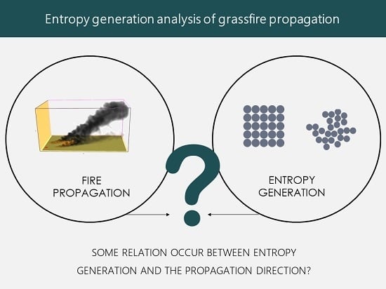
:Entropy generation is commonly applied to describe the evolution of irreversible processes, such as heat transfer and turbulence. These are both dominating phenomena in fire propagation. In this paper, entropy generation analysis is applied to a grassland fire event, with the aim of finding possible links between entropy generation and propagation directions. The ultimate goal of such analysis consists in helping one to overcome possible limitations of the models usually applied to the prediction of wildfire propagation. These models are based on the application of the superimposition of the effects due to wind and slope, which has proven to fail in various cases. The analysis presented here shows that entropy generation allows a detailed analysis of the landscape propagation of a fire and can be thus applied to its quantitative description.
1. Introduction
In the last decades, both entropy and entropy generation have been largely applied in engineering procedures aiming to improve the performances of manufactured devices [1,2] as well as and for modelling the behaviour of natural phenomena. When the entropy generation (i.e., the irreversibility) is minimized in properly constrained components and systems, their exergy destruction becomes minimal [3,4]. Engineering approaches based on this concept allow designing and operating devices and systems as efficiently as possible. Minimum entropy generation analysis has been applied to thermal insulation problems involving minimum heat transfer at fixed temperature difference and thermal enhancement involving minimum temperature difference to exchange a fixed heat flux [2]. In the literature, there are numerous applications of entropy generation analysis to storage systems [5,6,7], fluid flow within technical devices [8,9,10], engines [11,12], heat exchangers [13,14] and desalination plants [15].
More generally, many processes or phenomena that take place in Nature are known to occur in a way that minimizes or maximizes entropy production [2,16,17]. In [16], it is confirmed that the type of motion occurring while a fluid flows in a duct chooses is the one that assures maximum entropy generation (or minimum, depending on the constraints). Entropy is used for describing different phenomena involving both biological and inanimate systems, such as animal locomotion, vegetation, organ size, water basins and social organization [18,19]. As regards the discrepancy between the concepts of maximum and minimum entropy generation, in [20,21] it has been established that maximum entropy production principle can be considered as a direct consequence of minimum entropy generation. Among the processes obeying to the principle of maximum entropy generation there are radiation, convective heat transfer and turbulence [20]. All these phenomena are involved in grassfire evolution. The application of entropy generation analysis to fire propagation in vegetative fuels is thus expected to provide insights that can be used for predicting its evolution and eventually to fight it.
The available models for wildfire behaviour prediction can be classified in two main classes: empirical/semi-empirical models [22,23] and full physical models [24,25]. Models belonging to the first class are typically 1D models that are then extended to 2D landscape propagation through proper approaches. These models currently suffer from some limitations due to low accuracy while forecasting fire propagation [26]. In contrast, physical models are accurate, but they entail large computational costs and cannot be used as emergency management tools [27]. An analysis of possible relations between fire propagation and the entropy generation can be helpful in better understanding the physics of wildfire evolutions as well as to overcome possible limitations in empirical approaches. As an example, a vector addition approach is often used in order to obtain landscape (2D) propagations of fire front calculated through the Rothermel model (1D model). As reported in [28], such an approach is not sufficiently supported by experimental data and still requires investigation. This is especially true in case of flashover, where a sudden change in fire behaviour [29] is caused by the feedback effect due to the convective flow, which is provoked by the fire when wind or positive increasing slope act [28]. In such case, the superimposition of effects does not apply and thus conventional empirical approaches fail.
In this work, an entropy generation analysis has been performed in order to study fire propagation scenarios from a second law point of view. The main goal of the analysis is to investigate the links between entropy generation and wildfire propagation occur. In particular, the paper shows that entropy generation maximization can detect the directions of the wildfire propagation in an accurate way, without the intrinsic limitation associated to the linear combination of the different driving forces.
2. System Description
The system analysed in this work is an herbaceous field where a grass fire propagates starting from an ignition point source. This scenario is selected because it is the easiest to describe from a physical viewpoint, but the geometry and boundary conditions have been selected in order to properly highlight the features of the various models.
The considered domain is 32 m long, 16 m high and 16 m wide (see Figure 1). The ignition area is located in the south-west area, near the left bottom corner; this is a squared area with a surface of 1 m2. Initially, a heat source is imposed for about 30 s, with a Heat Release Rate (HHR) of 1 MW/m2. The domain dimensions and the ignition point location have been selected in order to efficiently catch the fire evolution in the direction where propagation is supposed to occur, due wind conditions and slope direction. The computational domain is 16 m high, to take into account the phenomena occurring in the air volume above the fire and the plume physics. The terrain slope cannot be seen in Figure 1, as it is imposed by adjusting the gravity vector components.
The terrain is covered with a homogenous herbaceous fuel with the following characteristics:
- height: 0.2 m (low/medium height)
- heat of combustion: 18,500 kJ/kg (typical value as indicated in [30])
- moisture content: 4% (very dry fuel)
- fuel load: 0.5 kg/m2 (medium/high load)
- char fraction: 10% (typical value)
- density of the vegetative fuel: 512 kg/m3 (typical value as indicated in [25])
- surface over volume ratio is 4950 m−1 (typical value for herbaceous fuel [31])
The wind spreads towards the East with an intensity of 2 m/s. The terrain is 18° slope, directed towards a direction between NE and N, so that an angle between wind and slope of 60° is obtained. As an effect, the main fire propagation will occur between E and N. Fire propagation analysis lasts 250 s, which is the time spent to reach the end of the domain.
3. Method
In order to investigate the relation between fire front propagation and entropy produced, three different approaches for fire simulation have been used, as indicated in Figure 2:
- (a)
- 3D full physical model (block 2). This plays the role of a field experiment;
- (b)
- entropy generation analysis (block 5). This is the proposed approach;
- (c)
- 1D model with a vector composition approach (block 8). This is the reference for comparing the proposed approach to, as it is a commonly adopted prediction method.
The full 3D physical model allows one to obtain a fire propagation close to the real one and it has been used for obtaining a numerical experiment with the same characteristics of a real fire experiment, but fully controlled. The model allows one capturing the temperature evolution in several points of the domain, similarly to the approach adopted in field experiments, where thermocouples are properly installed in the fuel [32]. The physical model is used in this work with two different purposes:
- collect temperature evolutions and the other data which are needed for calculating the various terms of entropy generation and setting the coefficients for the vector composition analysis (block 3);
- generate the reference terms (the fire propagation velocity) for comparing the results obtained through the compact models, i.e., the entropy generation approach and the vector composition approach (block 4).
The 1D model based on vector composition is used for comparing the entropy generation approach to a common approach for identify the fire front landscape evolution (block 10). The three models are detailed in Section 3.1, Section 3.2 and Section 3.3. Two fire front conditions are considered in the analysis:
- STATE 1: the fire front after 185 s, i.e., when the fire front is fully developed, is used for gathering data for entropy generation analysis and the vector composition analysis.
- STATE 2: the fire front after 230 s is used for comparing the results obtained through the three approaches.
3.1. Entropy Generation Analysis of a Grassland Fire Event
An unsteady process, which exchanges heat flux (Φ) and mass flow rates (G) with the surroundings, generates an entropy rate which is expressed by the second law of thermodynamics:
where ∑irr is the entropy generation, always positive [20]. The second law is applied here to a snapshot of the fire front propagation, using a lumped parameter approach. The hypothesis of homogeneity inside the control volume is assumed, therefore the mean values of the thermodynamic quantities are selected for describing each volume. For compatibility with this choice, small control volumes have been selected for the analysis. With respect to the approach usually considered in entropy generation minimization, which consists in the separate calculation of the terms associated to each physical phenomenon, indirect calculation performed through Equation (1) provides less detailed information, but requires much less data to be implemented. This feature makes the approach adopted here more suitable for application to fast predictive analysis.
The fire front at the STATE 1 has been divided into 26 equal parts, each corresponding to a control volume. Each volume presents the following characteristics:
- It is oriented with two faces parallel to the fire front.
- In each volume, a fictitious thermocouple is installed. This allows the detection of the temperature during propagation, providing information in the same way that would be available from an experimental campaign. The thermocouple sampling time, dtTH, is 0.25 s.
- The length l is selected as the space the front travels in a time equal to dtTH.
- Each control volume exchanges mass and energy with the surrounding through five control surfaces: two lateral surfaces, two frontal surfaces and the top surface. The latter is considered only for balancing the mass transport through a contribution which is always exiting the volume.
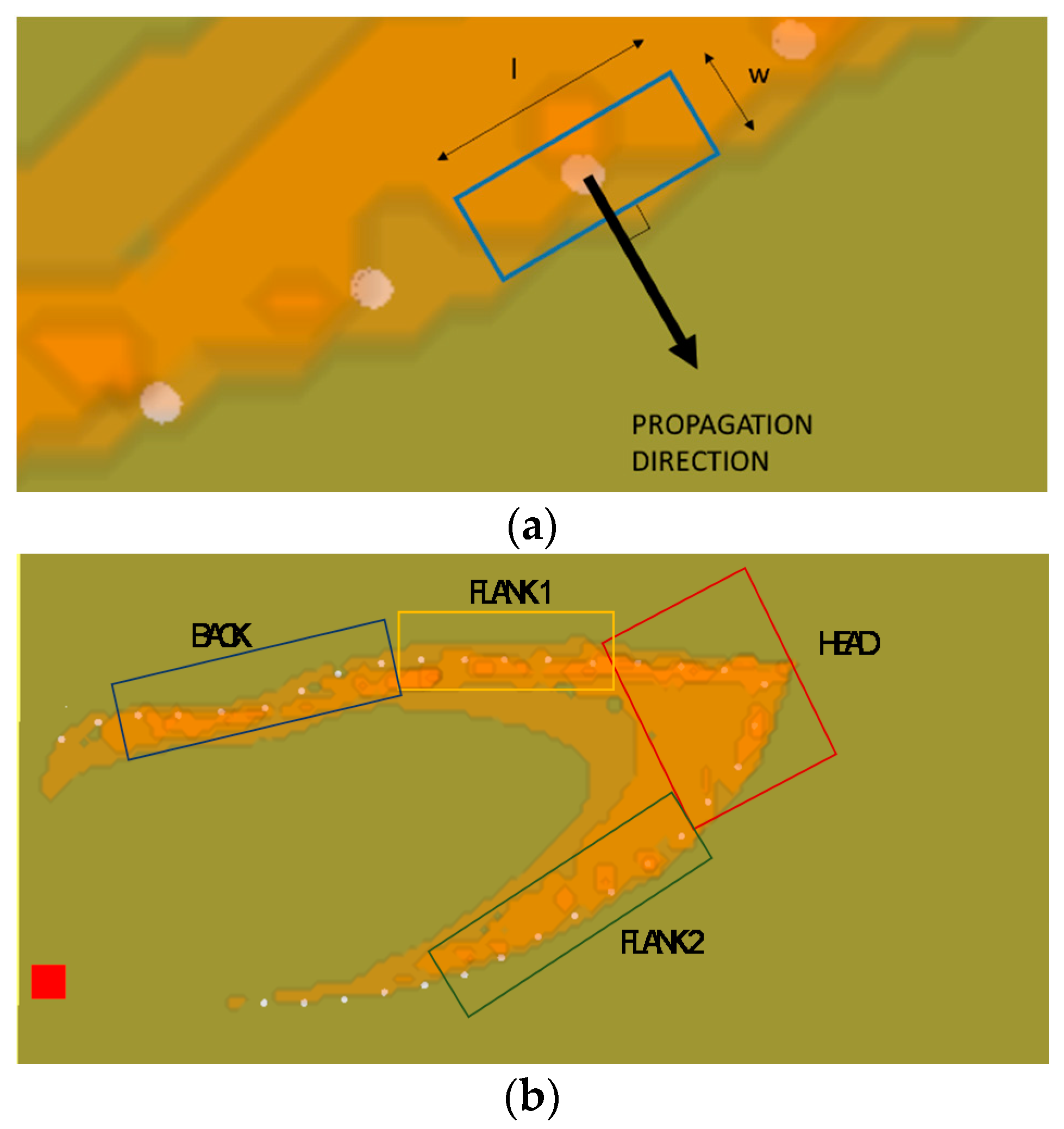
A schematic of a control volume characteristics is reported in Figure 3a.
The time considered for this analysis of a control volume is the entire period the flame takes to reach its central point. This is stopped at the time the first temperature peak occurs in the cell, i.e., when the beginning phase of combustion ends.
For a clearer explanation of the results, the fire front is divided into four main sectors, which are depicted in Figure 3b:
- Head, where wind and slope influence are high and the fire front propagates faster;
- Flanks (in particular Flank 1 and Flank 2), which are the sectors where the wind and slope contributions are smaller than at head;
- Back, which is the sector where the influence of wind and slope is negligible and the fire front proceeds slowly.
The analysis of these control volumes considers all the three terms described in Equation (1). The first term on the right-hand side of Equation (1) (TERM 1) includes the contribution of the heat flux that the control volume exchanges with the extern. Both the convective and radiative mechanisms are considered.
The radiative heat exchanged with the surroundings can be split in two main contributions. The first one occurs when the combustion region is reaching the thermocouples and the radiative flow is entering the control volume. This is physically described by Equation (2). The second contribution occurs when the fire is inside the control volume and the radiative flow exits (Equation (3)). The total radiative flux is thus obtained as the sum of the two function and (Equation (4)):
The convective heat exchange, due to the difference between the control volume temperature and the environment temperature Tenv, is evaluated as follows:
where A is the exchange surface and h is the convective heat exchange coefficient [32].
The second term on the right-hand side of Equation (1) (TERM 2), represents the entropy flux exiting (+) or entering (−) the control volume due to mass exchanges. These are due to the wind and buoyancy effects. The latter is caused by the up-slope terrain. In fire propagation, this contribution is usually treated as an equivalent wind speed [22,28]. The total convective velocity is thus the sum of the wind speed (v) and equivalent slope velocity (u) (Equation (6)):
The equivalent slope velocity is related to the slope angle β through the k slope coefficient.
An analysis for different values of wind and slope has been conducted and the corresponding ROSi has been thus collected in two different cases [33]:
- no-slope condition and wind velocity equal to
- no-wind condition and slope equal to
The kSLOPE coefficient is calculated by relating wind speed and slope angle through evaluation of the increase in the rate of spread (ROS) of the fire front that they produce, with respect to the no-wind and no-slope condition, namely:
The kSLOPE is the mean value of the various kSLOPE_i obtained for different slope angles (Equation (9)):
The mass flow rate entering and exiting the system are evaluated considering the effect of wind and slope velocity in all the faces of each control volume.
The evaluation of the specific entropy associated to the mass flow rates crossing the fire front can be performed if the temperature of air entering the system through all the five faces in each cell is known. For evaluating these values, two main assumptions are applied:
- An upwind scheme is considered. This implies that the temperature at the boundaries are assumed as the temperature in the upstream control volume.
- Travelling wave assumption for the fire front, considering that an idle condition has been reached. Such assumption is acceptable in the case of fully developed fire in a sufficiently homogeneous fuel. Temperature evolution in a cell is the same recorded at the previous cell, just shifted ahead in time of the period spent by the front to travel the distance between two points. The same assumption is made for the following cell, shifting the time back.
Temperature evolution at the forward and backward boundaries of a control volume i are evaluated by shifting of a certain amount of time the temperature collected by the ith thermocouple. The temperature evolution at the left and right boundaries are equal to the temperature evolution at the closest control volumes. In the case of the top surface, mass flow is always exiting through the plume. Its temperature is considered as that of fire.
The third term on the right-hand side of Equation (1) (TERM 3) represents the variation in entropy that occurs within the control volume during time evolution. This term can be written, neglecting pressure variations, as:
It should be recalled that the total entropy generated ∑irr is always positive, while the three terms can be either positive and negative, as calculation is performed through the second law in the form of Equation (1), instead of the direct calculation of the separate terms, which is the typical approach used in entropy generation minimization [2].
3.2. WFDS
The grassfire propagation is simulated through a 3D model, called Wildland Fire Dynamics Simulator (WFDS) [25,34]. WFDS is a 3D full physical simulator developed at the U.S. National Institute of Standards and Technology (NIST). The WFDS model is based on the governing equations for buoyant flow, heat transfer, combustion and the thermal degradation of vegetative fuels. Turbulence in the gas-phase is solved through a large eddy simulation (LES) approach). WFDS was validated for both a grassland fire evolution (the system considered in this work) in [25], and crown fires [34].
WFDS reads input parameters, domain description and computational details from a text file providing a time-dependent and three-dimensional prediction of the fire propagation. Furthermore, WFDS writes user-specified output into files; in particular, it is possible to collect temperature, velocity and other quantities in the selected points of the domain.
Wind speed is selected imposing a certain velocity to an open face while the upslope terrain is considered managing the gravity vector direction. The computational grid of the considered domain is characterized by 160 elements in the domain length, 80 elements on domain thickness and 80 elements on the domain height, all of them 0.2 m.
In order to perform the entire simulation, lasting 250 s, about 30 h are required on a single 3.3 GHz CPU. It is therefore clear that such kind of models cannot be used as operational tool for managing emergencies, because of the very high computational time required, as mentioned in [27].
Temperature evolutions are monitored through a virtual installation of sensors in the points reached by the fire front at t = t1 = 185 s (STATE 1). 26 fictitious thermocouples, corresponding to as many control volumes, have been installed along the fire front. A preliminary simulation has been performed in order to catch the grassfire front position at time t1 for selecting the control volumes and correctly locate them and the thermocouples inside each volume.
3.3. Vector Composition Propagation
A common approach to obtain landscape evolution of wildland fires consists in applying a 1D model, usually the Rothermel model, in various points of the fire front. Contributions due to wind and slope can be composed together as vector composition.
A simple physical model, based on the mass and energy equation, is here used in order to obtain the propagation velocity on a specified direction. This model is described by Equations (11)–(14). Several similar models can be found in the literature [35,36,37,38]:
Values for quantities a (mass loss coefficient), λ (equivalent thermal conductivity associated with the mixture of fuel and air) and h (heat losses coefficient) have been evaluated trough an analysis of the temperature evolution, as explained in [32].
The term w shows how wind and slope in a specific direction are summed together. The term g, accounts for the convective heat losses towards the environment, the heat gained by the fuel combustion and the radiative heat exchange with the surrounding.
The radiative term is computed as:
The coefficient r, has been evaluated with the same approach for coefficients a, λ and h.
Mass balance is based on the assumption of burning mass rate proportional to the amount of fuel (Equation (12)), as made in similar works in literature [35,36,37,38]. The mass loss parameter assumes non-zero values only if the fuel is burning, i.e., the cell temperature at the previous time step is higher than the ignition temperature.
The presence of the radiative term (3) makes the energy equation non-linear and dependent on the terrain slope. The problem is discretized through a finite difference implicit approach, and solved through a Newton-Raphson algorithm. For further details see [32].
3.4. Fire Evolution Comparison
Entropy generated during the propagation process does not provide itself a measure of the rate of spread, but it gives information of the expected shape of the fire at the following time step. Therefore, the ratio of the propagation velocity of each section respect to the others is converted into a rate of spread interpolating results on the basis of the actual rate of spread. This evaluation has been performed through a proper coefficient, the equivalent ROS factor, evaluated as follows:
where n is the total number of cells and ROSWFDS the rate of spread obtained through WFDS. The coefficient μ is used for obtaining the fire front in the STATE 2 through entropy generation, following Equation (17):
The same approach has been used in order to correct the ROS obtained through the 1D physical model, which can be affected by inaccuracy for the simpler physical problem description. The ROS obtained are applied to each point of the fire front considering, as usually done for fire propagation analysis, the punctual propagation direction as perpendicular to the fire front in that point.
4. Results
4.1. Pre-Processing Results
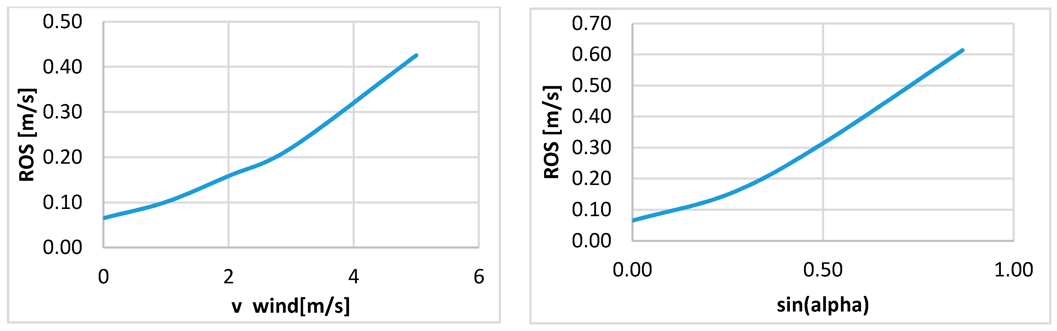
Results obtained during the preliminary WFDS simulation are used for the evaluation of the coefficient relating the terrain slope and a fictitious wind velocity (kSLOPE). Figure 4 shows the ROS obtained varying the wind speed in no-slope condition and varying the slope in no-wind condition. The relation between ROS and both the wind speed and the slope are not so far from linearity in the region of slow fire propagation. The combined analysis of these results allows finding, through the Equations (7)–(9), the kSLOPE value. A value of kSLOPE equal to 6.9 can be considered valid for the ranges: wind 0–5 m/s and slope 0–45°.
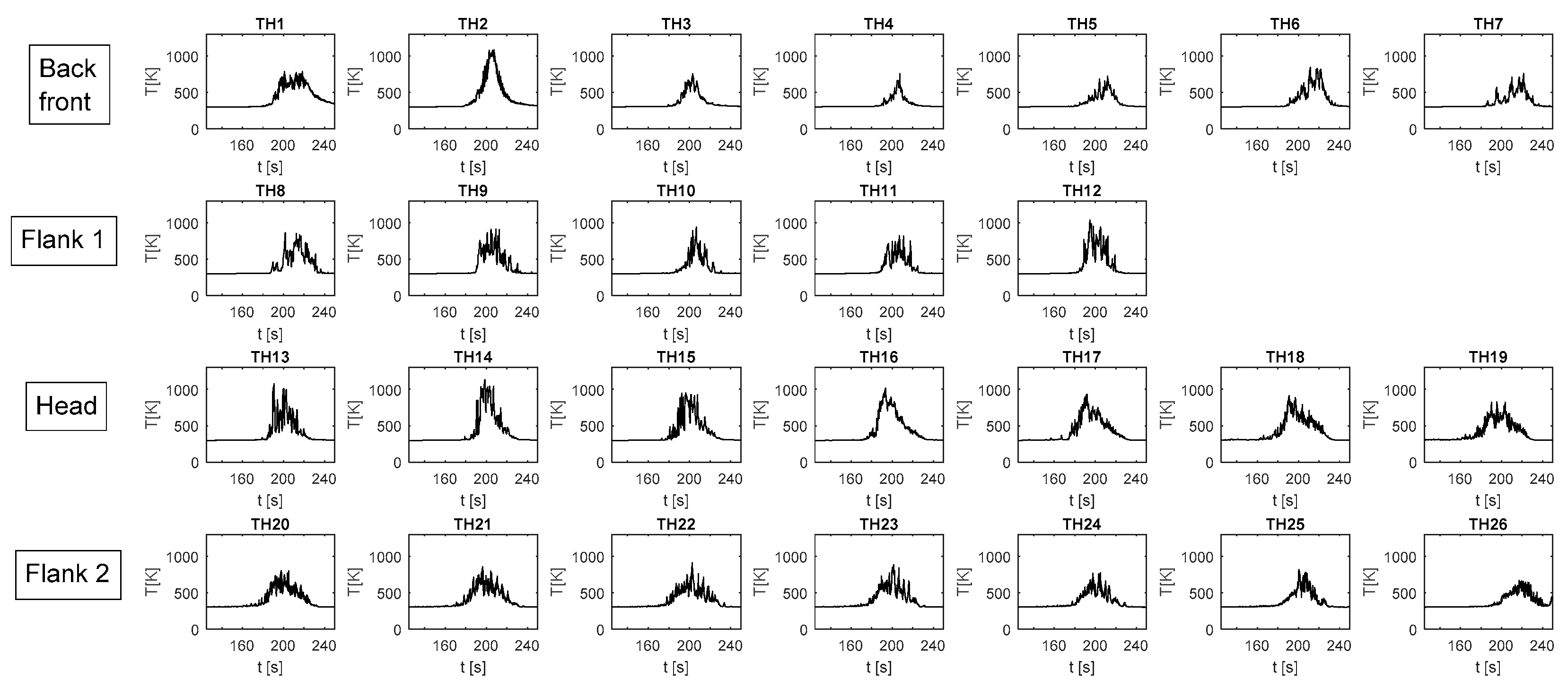
In Figure 5 it is possible to observe the 26 temperature evolutions collected by the thermocouples installed in the control volumes during the entire simulation. The combustion region reaches the cell where the thermocouples are installed after about 185 s. The temperature evolutions present some similarities and various differences. All the temperature evolutions are characterized by strong fluctuations, which are indicative of the high turbulence phenomena occurring during the fire propagation [39].
The maximum values reached during the evolution fluctuates between 700 K and 1100 K. The maximum temperature in the points at the back sector of the fire front, is, on average, lower. In the head sector the temperatures assume a fuzzy and steep increase when the front is approaching. The passage of the flame lasts about 20–40 s depending on the cells.
4.2. Main Entropy Generation Results
At first, the three terms of the entropy balance forming the total entropy generation rate have been analysed independently. Figure 6 shows the evolutions of these terms in 4 different points, one for each of the front sector reported in Figure 3b.
TERM 1 is zero when the difference between the cell temperature and the environmental temperature is zero and no flame is approaching. TERM 1 increases with increasing the control volume temperature. In the section where the temperature is higher than the environment and a certain amount of heat exits the system, the irreversibility generated by the losses follows Equation (18):
where the three constant a, b and d are defined as follows:
The main contribution on the overall entropy generated by thermal losses during propagation is due to convection. This is shown in Figure 7a, which reports the entropy generation due to convection and radiation during the process. According to the assumptions, convection mainly dominates the heat dissipation. In particular, convective losses are higher in the cells located in Flank 2, because it is near the ignition in the direction the wind spreads. This produce a slightly increase in the temperature inside the control volume and, with respect to all the other sectors, in these cells higher convective losses occur.
Going back to Figure 6, the entropy generation due to mass flow rates is zero in the case of no wind and no slope (and therefore the equivalent wind velocity is zero) and when the surrounding cells are at the same temperature of the cell. The highest values are obtained in the head front sector, where the total equivalent velocity is very high due to the cell orientation, which is strongly affected by slope and wind contributions. The curve representing the evolution of this term is very fuzzy, particularly at the head of the front. This shape is due to the significant temperature difference between the cell and the surrounding cells. Figure 7b reports the contributions of the mass flow rates crossing the control volume from the front (“l” in Figure 3a) and lateral (“w” in Figure 3a) faces of the cells. Irreversibility is higher in frontal faces, mainly due to their larger area, with respect to the front faces, which causes a higher mass flow rate. In particular, mass flow rates are higher in the cells that are mainly affected by the equivalent wind direction (roughly spreading between E and NNE). No particular trend is detected in the irreversibility produced through the lateral faces. This mainly depends on the difference between the temperature at the cell and at the neighbour cells.
Regarding TERM 3 in Figure 6, which represents the irreversibility evolution due to entropy variation within the control volume, the differences between the various sectors only depends on the temperature variation in each time-step. The maximum values reached are considerably lower than those related to TERM 1 and TERM2.
The integrals of the curve represented in Figure 6 are evaluated and results are reported in Figure 8 for all the considered values. Bars represent the total entropy generated during the entire process (until the first temperature peak).
The values of TERM 1 significantly differ in the various sectors of the front. In particular, the largest values occur in the second flanks of the fire front, because of the higher temperature gradients.
The contributions due to mass transfer (TERM 2) are larger at the head of the fire front. This is particularly relevant for the point at the tip of the front (the point characterized by a larger y coordinate). Values are negative at the end of the lower front, due to two reasons: (1) in these cells the fire front propagates in a direction that is opposite with respect to the direction where the equivalent velocity spreads and (2) the entropy flux exchanged by the lateral surfaces is lower than zero.
TERM 3 is quite similar in the various cells. Such values mainly depends on the temperature variation inside the control volume during the considered time. This varies between the environmental temperature and the first peak temperature. Consequentially the cells characterized by higher entropy generation are the ones in the central part of the fire front, where temperature rapidly increases when reached by the fire front.
It is evident that TERM 3 is negligible compared to the contribution due to mass flow rate and heat exchanged. TERM 2 in the central part of the fire front includes some values of the same magnitude as the ones of the TERM 1 and more than ten times the TERM 3. If all the control volumes are considered, the mean contribution due to mass flow rate and the one due to the losses are quite similar (about 250 J/K).
4.3. Propagation Prediction Comparison
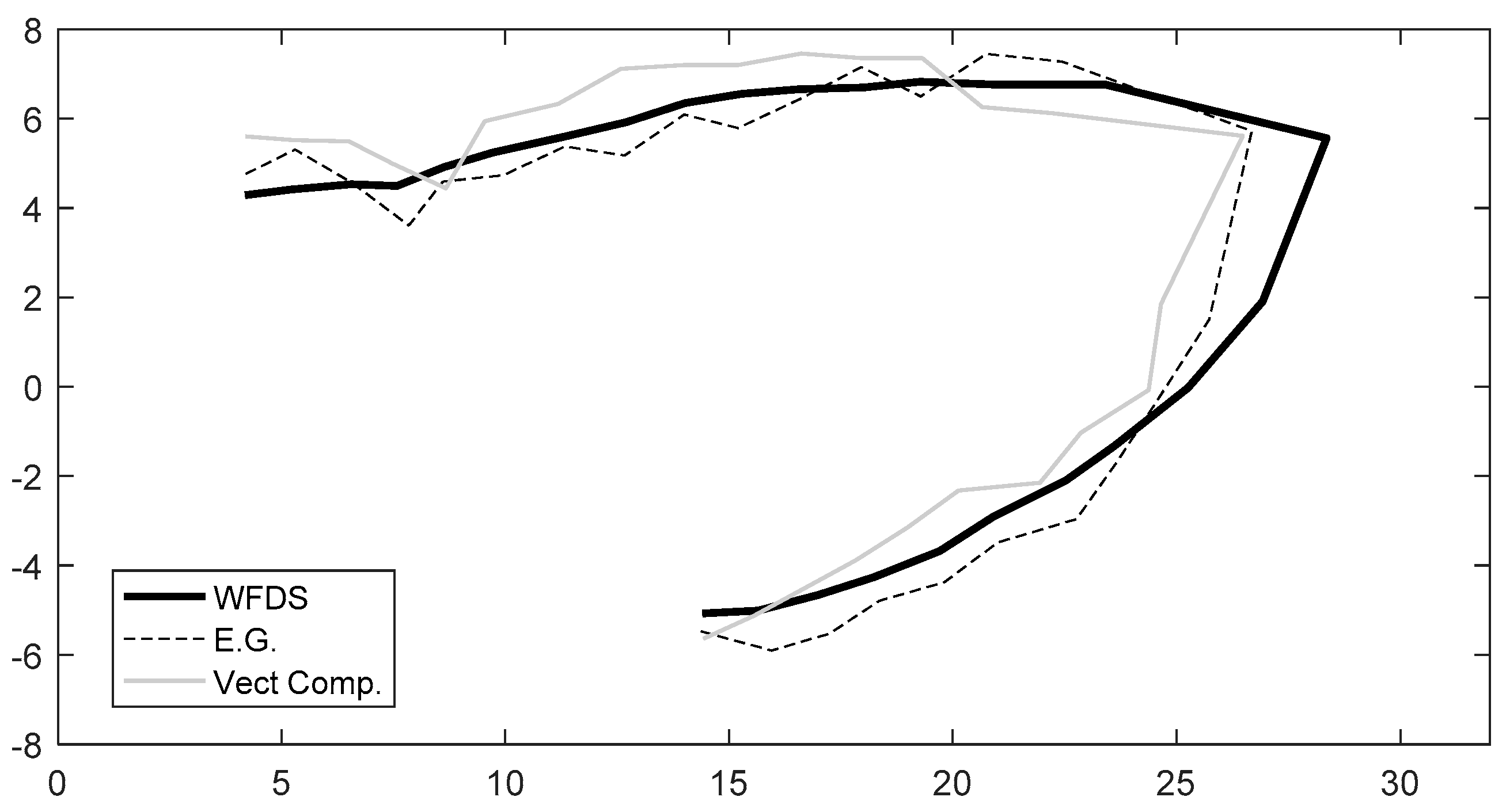
Using the methodology described in Section 2, the evolution predictions for the STATE 2 are obtained for all the discussed approaches. Results are shown in Figure 9. The capability of the compact models in predicting the fire evolution can be evaluated through comparison of the corresponding fronts (plain line for the vector composition and dashed line for the entropy generation) with the results of the full physical model (bold line).
The vector composition tends to overestimate the upper flank propagation while it underestimates the faster sectors. In particular, the error performed in terms of mean distance with respect to the “real” front is about 0.8 m.
The entropy generation approach detects the fire propagation quite accurately. This approach allows one reducing the average deviation to about 0.6 m. The main inaccuracy in the prediction through the entropy generation (and through the vector composition) is represented by the position of the tip (for tip it is intended the point with the largest x coordinate, where the propagation is maximum). This is due to the fact that, in the WFDS simulation results, propagation in that point does not proceed perfectly perpendicular to the control volume selected on the tip. The discretization performed should be finer at the head of the fire front if the goal is a precise evaluation of the tip propagation.
Uncertainties that affect the rate of spread at the head of the fire have been computed for both entropy generation and vector composition approach. The mean relative error is 17% in case of entropy generation and about 30% if vector composition is used. This result shows that entropy generation provides the fire propagation prediction with a more precise head front estimation.
4.4. Discussion
The lumped parameter approach allows one evaluating the overall amount of entropy generated with little information at disposal, which is a requirements for the possible application to real fires. This approach has been already applied to investigate the evolution of entropy generation with increasing wind speed and ground slope [33]. In that paper [33] it is shown that the total entropy generated is minimal when no wind and slope take place and increases when the slope or the wind speed raise (and therefore a faster fire propagation occurs). In this work the two driving forces have been applied together in order to investigate their combined effect, which is a criticality in the case of empirical or semi-empirical modelling. Fully physical modelling shows that heat transfer plays also an important role. This is confirmed by specific experimental works, such as [40]. In the case of the application presented in this work, the flanks present such characteristics. Here the use of equivalent velocities does not capture the fire evolution properly, resulting in an overestimation or underestimation of the propagation velocity, depending on the relative orientation of the fire line and the equivalent velocity. In contrast, the entropy generation analysis allows an evaluation of the driving forces from a thermodynamically consistent way. Heat fluxes and temperature gradients are directly considered in the model, thus permitting a better description of the physical phenomena even if in a compact form. Various assumptions are formulated in the model, in particular:
- (1)
- The fire propagation is considered as a travelling wave. This is a limitation in the case of significantly non homogenous fuels.
- (2)
- Each cell is described though the mean values of the thermodynamic quantities. This makes the results dependent on the size of the control volume. In particular, this is crucial when the tip of the fire front is examined.
Further understanding of the propagation mechanisms can be obtained through implementation of a direct calculation of the entropy generation terms. Nevertheless, this requires significant amount of information which can be obtained, for instance, from properly instrumented unmanned aerial vehicles (UAVs) in field experiments but it is nowadays difficult to obtain in real fires. As regards computational cost required, the simulation through WFDS, entropy generation and 1D model, requires respectively 30 h, 10 s and about 1 min on a single 3.3 GHz CPU. This means that the proposed approach.
5. Conclusions
In this paper, an entropy generation analysis of a grass land fire event is proposed with the aim of understanding the relation between the entropy produced during the fire propagation and the front evolution. Three different approaches have been used for simulating the fire propagation:
- (a)
- A 3D model able to accurately predict the fire evolution. This model is used to provide the necessary data for tuning the parameters of other approaches. In addition, it provides the reference fire front propagation to be used as a term of comparison for the other approaches.
- (b)
- An entropy generation approach, which provides the entropy generated in all the control volumes along the propagating fire front.
- (c)
- A 1D model using, as the convective velocity, the vector resulting from the summation of the wind and slope contributions.
All the approaches have been applied to a grassland fire evolution, in order to predict the evolution occurring during a certain time span.
The entropy generation approach and the corresponding results have been deeply detailed. The main contributions in terms of entropy generation are constituted by those associated with the mass flow rates crossing the control volumes and the heat exchanged. Mass flow rates contribution is more significant where fire propagates faster while the heat transfer more contributes in the other sections, particularly at the flanks of the front. The latter is not negligible and constitutes a major difference with respect to conventional approaches based on velocity vector compositions.
In the end, the comparison of entropy generation and vector composition approach for the grassfire evolution prediction is presented. The comparison shows that entropy generation approach allows detecting the fire front at a future time with slightly higher precision than the vector composition approach. Entropy generation shows to be a quantity deeply related to the fire propagation, more than the simple equivalent velocity. This is particularly evident in the areas of the fire front where the contributions due to heat transfer are relevant. The insights provided by this work can constitute the ground base for developing fast prediction tools to be used during operation, such as to evaluate possible risks for the operators, plan effective fire attacks, take decisions about people evacuation or implement possible protections to critical infrastructures.
Acknowledgments
Work conducted within the European Project AF3—Advanced Forest Fire Fighting. FP7 THEME [SEC-2013.4.1-6] Preparedness for and management of large scale forest fires. Grant agreement No. 607276.
Author Contributions
The work has been developed in team. Both the authors take part to the study conception and the design of the methodology used in the work. Elisa Guelpa worked on performing the analysis and she wrote the first draft version of the manuscript while Vittorio Verda critically revised the work performed in all the phases and the manuscript.
Conflicts of Interest
The authors declare no conflict of interest.
Nomenclature
| A | area (m2) |
| c | specific heat (J∙kg−1∙K−1) |
| F | view factor |
| G | mass flow rate (kg∙s−1) |
| g | heat generation contribution (W∙m−3) |
| d | fuel height (m) |
| h | convective transfer coefficient, (W∙m−2∙K−1) |
| k | equivalent slope velocity coefficient (m) |
| l | length (m) |
| m | mass (kg) |
| N | number of cells |
| R | radiative heat exchange coefficient |
| r | equivalent propagation term |
| t | time (s) |
| T | temperature (°C) |
| s | specific entropy (J∙kg−1∙K−1) |
| S | entropy (W∙K−1) |
| u | equivalent slope velocity (m) |
| v | wind velocity (m∙s−1) |
| V | total velocity (m) |
| w | width (m) |
| Greek letters | |
| β | slope angle |
| γ | convective coefficient |
| ε | emissivity |
| λ | equivalent thermal conductivity |
| 𝜇 | equivalent ROS factor |
| ρ | density |
| σ | Stefan-Boltzmann (W∙m−2∙K−4) |
| ∑ | entropy flux (W∙K−1) |
| Φ | heat exchanged (W) |
| ω | convective wind speed |
| Subscripts | |
| max | maximum |
| env | environmental |
| 1 | related to the first fire front |
| 2 | related to the second fire front |
| rad | radiative |
| conv | convective |
References
- Sciacovelli, A.; Verda, V.; Sciubba, E. Entropy generation analysis as a design tool—A review. Renew. Sustain. Energy Rev. 2015, 43, 1167–1181. [Google Scholar] [CrossRef]
- Bejan, A. Entropy Generation Minimization: The Method of Thermodynamic Optimization of Finite-Size Systems and Finite-Time Processes; CRC Press: Boca Raton, FL, USA, 1995. [Google Scholar]
- Gouy, G. Sur l’énergie utilizable (on usable energy). J. Phys. 1889, 11, 501–518. [Google Scholar]
- Stodola, A. Die Kreisprozesse der Gasmaschine. Z. VDI 1898, 506, 1086–1091. [Google Scholar]
- Guelpa, E.; Sciacovelli, A.; Verda, V. Entropy generation analysis for the design improvement of a latent heat storage system. Energy 2013, 53, 128–138. [Google Scholar] [CrossRef]
- Sciacovelli, A.; Guelpa, E.; Verda, V. Second law optimization of a PCM based latent heat thermal energy storage system with tree shaped fins. Int. J. Thermodyn. 2014, 17, 145–154. [Google Scholar] [CrossRef]
- Jegadheeswaran, S.; Pohekar, S.D.; Kousksou, T. Exergy based performance evaluation of latent heat thermal storage system: A review. Renew. Sustain. Energy Rev. 2010, 14, 2580–2595. [Google Scholar] [CrossRef]
- Sahin, A.Z.; Ben-Mansour, R. Entropy generation in laminar fluid flow through a circular pipe. Entropy 2003, 5, 404–416. [Google Scholar] [CrossRef]
- Schmandt, B.; Herwig, H. Diffuser and nozzle design optimization by entropy generation minimization. Entropy 2011, 13, 1380–1402. [Google Scholar] [CrossRef]
- Yapici, H.; Kayatas, N.; Kahraman, N.; Bastürk, G. Numerical study on local entropy generation in compressible flow through a suddenly expanding pipe. Entropy 2005, 7, 38–67. [Google Scholar] [CrossRef]
- Nakonieczny, K. Entropy generation in a diesel engine turbocharging system. Energy 2002, 27, 1027–1056. [Google Scholar] [CrossRef]
- Rakopoulos, C.D.; Kyritsis, D.C. Comparative second-law analysis of internal combustion engine operation for methane, methanol, and dodecane fuels. Energy 2001, 26, 705–722. [Google Scholar] [CrossRef]
- Giangaspero, G.; Sciubba, E. Application of the entropy generation minimization method to a solar heat exchanger: A pseudo-optimization design process based on the analysis of the local entropy generation maps. Energy 2013, 58, 52–65. [Google Scholar] [CrossRef]
- Shiba, T.; Bejan, A. Thermodynamic optimization of geometric structure in the counterflow heat exchanger for an environmental control system. Energy 2001, 26, 493–512. [Google Scholar] [CrossRef]
- Mistry, K.H.; McGovern, R.K.; Thiel, G.P.; Summers, E.K.; Zubair, S.M.; Lienhard, J.H. Entropy generation analysis of desalination technologies. Entropy 2011, 13, 1829–1864. [Google Scholar] [CrossRef] [Green Version]
- Paulus, D.M.; Gaggioli, R.A. Some observations of entropy extrema in fluid flow. Energy 2004, 29, 2487–2500. [Google Scholar] [CrossRef]
- Baldwin, R.A. Use of maximum entropy modeling in wildlife research. Entropy 2009, 11, 854–866. [Google Scholar] [CrossRef]
- Bejan, A.; Lorente, S. The constructal law of design and evolution in nature. Philos. Trans. R. Soc. B Biol. Sci. 2010, 365, 1335–1347. [Google Scholar] [CrossRef] [PubMed]
- Bejan, A.; Lorente, S. Constructal law of design and evolution: Physics, biology, technology, and society. J. Appl. Phys. 2013, 113, 151301. [Google Scholar] [CrossRef]
- Martyushev, L.M.; Seleznev, V.D. Maximum entropy production principle in physics, chemistry and biology. Phys. Rep. 2006, 426, 1–4. [Google Scholar] [CrossRef]
- Lucia, U. Maximum or minimum entropy generation for open systems? Phys. A Stat. Mech. Appl. 2012, 391, 3392–3398. [Google Scholar] [CrossRef]
- Rothermel, R.C. A Mathematical Model for Predicting Fire Spread in Wildland Fuels; Intermountain Forest and Range Experiment Station: Ogden, UT, USA, 1972. [Google Scholar]
- McArthur, A.G. Weather and Grassland Fire Behaviour; Forestry and Timber: Canberra, Australia, 1966; p. 23. [Google Scholar]
- Morvan, D.; Méradji, S.; Accary, G. Physical modelling of fire spread in grasslands. Fire Saf. J. 2009, 44, 50–61. [Google Scholar] [CrossRef]
- Mell, W.; Jenkins, M.A.; Gould, J.; Cheney, P. A physics based approach to modeling grassland fires. Int. J. Wildland Fire 2007, 16, 1–22. [Google Scholar] [CrossRef]
- Cruz, M.G.; Alexander, M.E. Uncertainty associated with model predictions of surface and crown fire rates of spread. Environ. Model. Softw. 2013, 47, 16–28. [Google Scholar] [CrossRef]
- Sullivan, A.L. Wildland surface fire spread modelling, 1990–2007. 1: Physical and quasi-physical models. Int. J. Wildland Fire 2009, 18, 349–368. [Google Scholar] [CrossRef]
- Viegas, D.X. Slope and wind effects on fire propagation. Int. J. Wildland Fire 2004, 13, 143–156. [Google Scholar] [CrossRef]
- Viegas, D.X.; Simeoni, A. Eruptive behaviour of forest fires. Fire Technol. 2011, 47, 303–320. [Google Scholar] [CrossRef] [Green Version]
- Albini, F.A. Estimating Wildfire Behavior and Effects; U.S. Department of Agriculture, Forest Service, Intermountain Forest and Range Experiment Station: Ogden, UT, USA, 1976.
- Scott, J.H.; Burgan, R.E. Standard Fire Behavior Fuel Models: A Comprehensive Set for Use with Rothermel’s Surface Fire Spread Model; U.S. Department of Agriculture, Forest Service, Rocky Mountain Research Station: Fort Collins, CO, USA, 2005.
- Guelpa, E.; Sciacovelli, A.; Verda, V.; Ascoli, D. Faster prediction of wildfire behaviour by physical models through application of proper orthogonal decomposition. Int. J. Wildland Fire 2016, 25, 1181–1192. [Google Scholar] [CrossRef]
- Guelpa, E.; Verda, V. Second law analysis of wind and slope contributions in grassfires. In Proceedings of the 9th International Exergy, Energy and Environment Symposium, Split, Croatia, 14–17 May 2017. [Google Scholar]
- Mell, W.; Maranghides, A.; McDermott, R.; Manzello, S.L. Numerical simulation and experiments of burning douglas fir trees. Combust. Flame 2009, 156, 2023–2041. [Google Scholar] [CrossRef]
- Simeoni, A.; Santoni, P.A.; Larini, M.; Balbi, J.H. On the wind advection influence on the fire spread across a fuel bed: Modelling by a semi-physical approach and testing with experiments. Fire Saf. J. 2001, 36, 491–513. [Google Scholar] [CrossRef]
- Balbi, J.H.; Santoni, P.A.; Dupuy, J.L. Dynamic modelling of fire spread across a fuel bed. Int. J. Wildland Fire 2000, 9, 275–284. [Google Scholar] [CrossRef]
- Santoni, P.A.; Balbi, J.H.; Dupuy, J.L. Dynamic modelling of upslope fire growth. Int. J. Wildland Fire 2000, 9, 285–292. [Google Scholar] [CrossRef]
- Guelpa, E.; Sciacovelli, A.; Verda, V.; Ascoli, D. Model reduction approach for wildfire multi-scenario analysis. In Proceedings of the VII International Conference on Forest Fire Research, Coimbra, Portugal, Peninsula, 14–21 November 2014. [Google Scholar]
- Silvani, X.; Morandini, F. Fire spread experiments in the field: Temperature and heat fluxes measurements. Fire Saf. J. 2009, 44, 279–285. [Google Scholar] [CrossRef]
- Raposo, J.; Viegas, D.X.; Xie, X.; Almeida, M.; Naian, L. Analysis of the Jump Fire Produced by the Interaction of Two Oblique Fire Fronts: Comparison between Laboratory and Field Cases. 2014. Available online: http://hdl.handle.net/10316.2/34013 (accessed on 21 August 2017).
Figure 1.
System illustration.
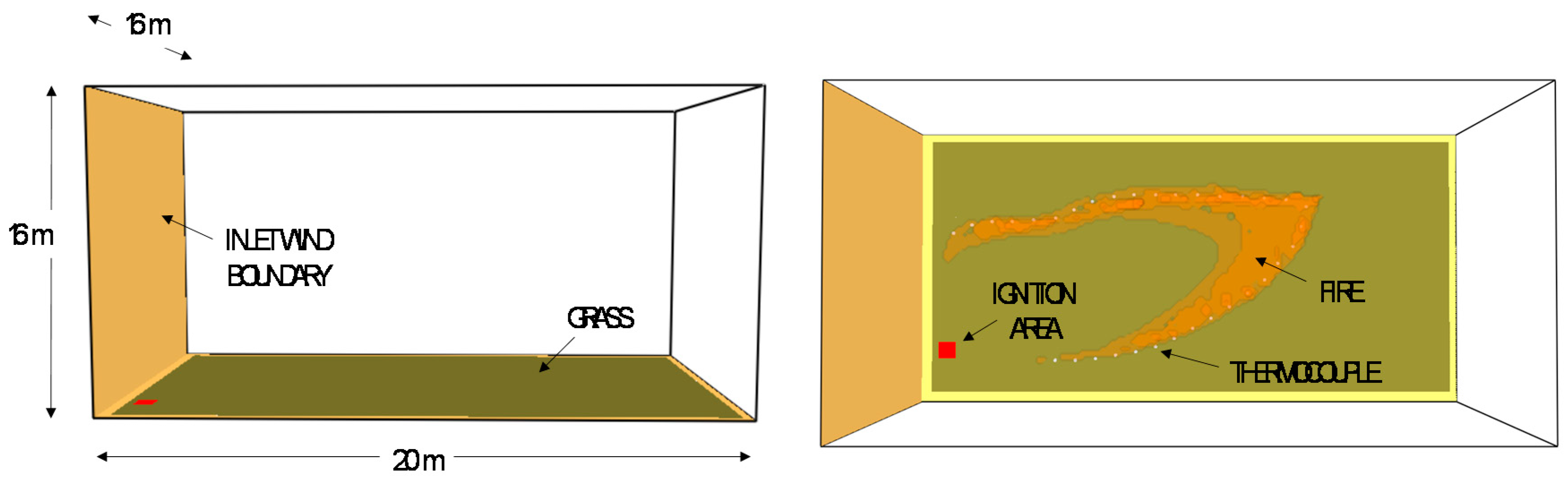
Figure 2.
Comparison between landscape propagation models.
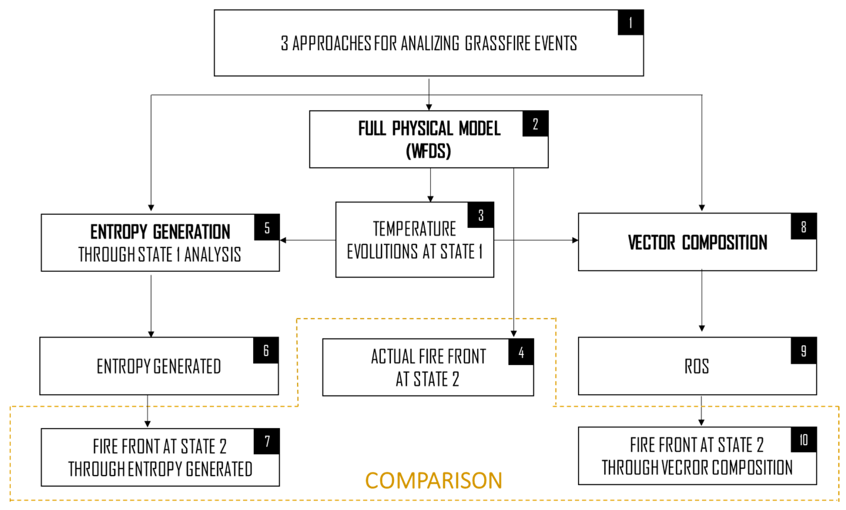
Figure 3.
(a) Control volume example; (b) Main fire front sectors.

Figure 4.
WFDS simulation results for different slope and wind speed.

Figure 5.
WFDS simulation results. Temperature evolution at the 26 thermocouple at STATE 1.

Figure 6.
Entropy flux generated evolution: three contributions.

Figure 7.
(a) Entropy generated through convection and radiation; (b) Entropy generated through the frontal and the lateral faces.
Figure 7.
(a) Entropy generated through convection and radiation; (b) Entropy generated through the frontal and the lateral faces.
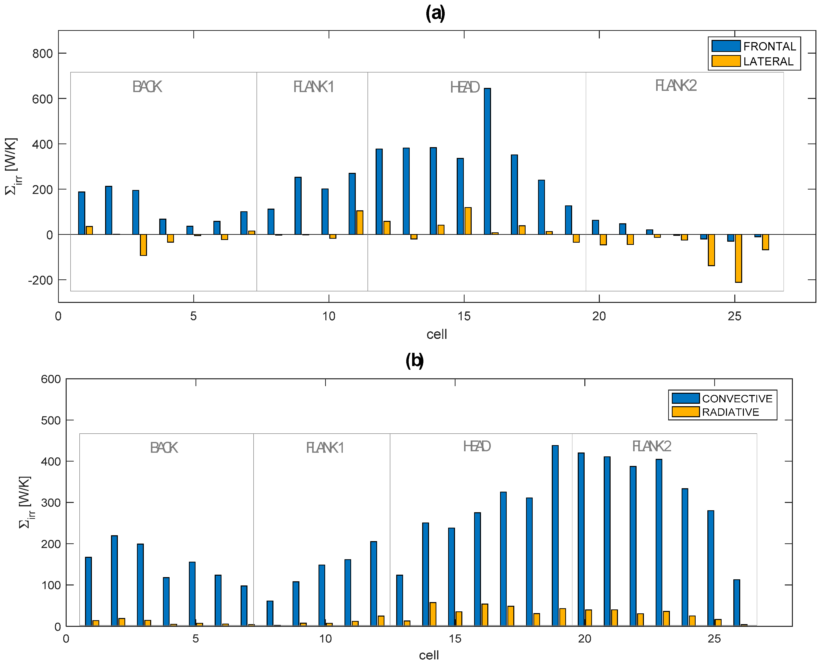
Figure 8.
Entropy generated: three contributions.
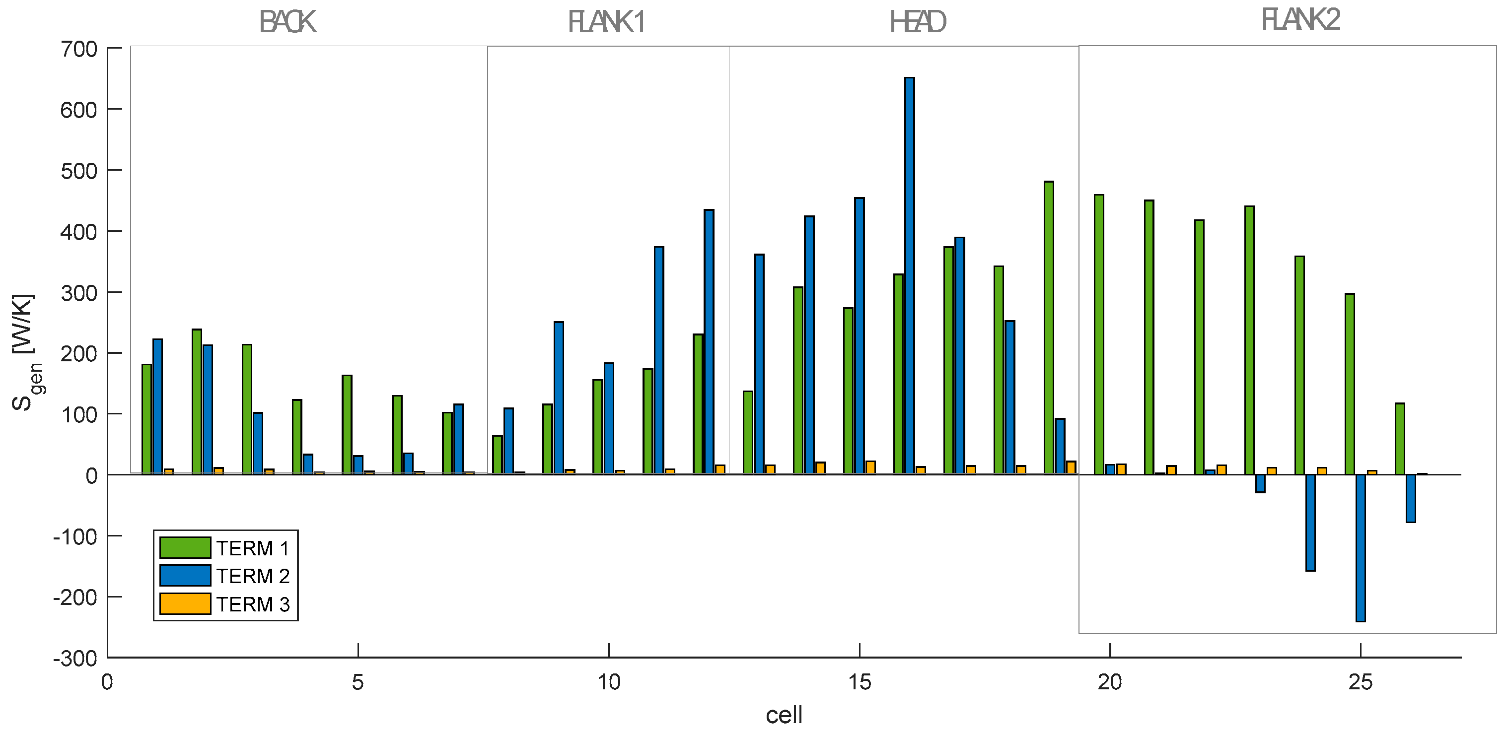
Figure 9.
Fire front prediction for STATE 2 through the different analyzed approaches. bold line = fire front; dashed line = entropy generation; grey line = vector composition.
Figure 9.
Fire front prediction for STATE 2 through the different analyzed approaches. bold line = fire front; dashed line = entropy generation; grey line = vector composition.

© 2017 by the authors. Licensee MDPI, Basel, Switzerland. This article is an open access article distributed under the terms and conditions of the Creative Commons Attribution (CC BY) license (http://creativecommons.org/licenses/by/4.0/).
Share and Cite
MDPI and ACS Style
Guelpa, E.; Verda, V. Entropy Generation Analysis of Wildfire Propagation. Entropy 2017, 19, 433. https://doi.org/10.3390/e19080433
AMA Style
Guelpa E, Verda V. Entropy Generation Analysis of Wildfire Propagation. Entropy. 2017; 19(8):433. https://doi.org/10.3390/e19080433
Chicago/Turabian StyleGuelpa, Elisa, and Vittorio Verda. 2017. "Entropy Generation Analysis of Wildfire Propagation" Entropy 19, no. 8: 433. https://doi.org/10.3390/e19080433
Note that from the first issue of 2016, this journal uses article numbers instead of page numbers. See further details here.