Robust Automatic Modulation Classification Technique for Fading Channels via Deep Neural Network

Abstract

In this paper, we propose a deep neural network (DNN)-based automatic modulation classification (AMC) for digital communications. While conventional AMC techniques perform well for additive white Gaussian noise (AWGN) channels, classification accuracy degrades for fading channels where the amplitude and phase of channel gain change in time. The key contributions of this paper are in two phases. First, we analyze the effectiveness of a variety of statistical features for AMC task in fading channels. We reveal that the features that are shown to be effective for fading channels are different from those known to be good for AWGN channels. Second, we introduce a new enhanced AMC technique based on DNN method. We use the extensive and diverse set of statistical features found in our study for the DNN-based classifier. The fully connected feedforward network with four hidden layers are trained to classify the modulation class for several fading scenarios. Numerical evaluation shows that the proposed technique offers significant performance gain over the existing AMC methods in fading channels.

1. Introduction

In digital communications, a task of classifying a modulation class from the received signal is referred to as automatic modulation classification (AMC) [1,2,3,4]. While conventional communication systems use training signal or control channels to provide the information on the modulation type to the receiver, there are some scenarios where such information is not available and thus the modulation type should be blindly estimated from the received data. Such scenarios often occur in signal intelligence in military applications, signal sensing for cognitive radio systems, and inter-cell interference cancellation for cellular communications. Since the receiver does not have the knowledge on which data symbols have been sent from the transmitter, it is challenging to classify the modulation type solely based on the received data samples.

The previous AMC techniques can be roughly divided into two categories. The first approach is to build a probabilistic model for the received signal and classify a modulation class based on some optimality criterion such as maximum likelihood function. Though these methods offer optimal detection performance for the given model, its classification accuracy degrades in the presence of model mismatch. In addition, the model-based approach needs the knowledge on various model parameters, which requires substantial computational complexity. The alternative approach is the machine learning-based approach, where the machine is trained to classify the modulation type based on the training data in off-line and then the trained machine is deployed to apply to the real data. Assuming that the test data is sampled from the same distribution as that of the training data, the machine learning-based methods yield satisfactory classification performance without the exact knowledge of the system model. Since machine learning-based method is simple to design and robust to model mismatch, we are mainly concerned with this approach in this paper.

In general, two key steps should be performed for the machine learning-based AMC: (1) feature extraction step and (2) classification step. Widely used features for AMC include the variance of signal magnitude, frequency, and phase, wavelet coefficients and high order statistics such as cumulants [5,6,7,8]. After extracting the features, the classifier is applied to decide which class they belong to. So far, various kinds of classifiers have been used, including decision tree [5,7,9], support vector machine (SVM) [8,10,11], and artificial neural network (ANN) [12,13]. While these works have mostly focused on AMC task under additive white Gaussian noise (AWGN) channels, there exist only a few works presenting the AMC system designed for fading channels [14].

In this paper, we introduce an enhanced AMC technique based on deep neural network (DNN). First, we analyze the effectiveness of the extensive list of the statistical features for fading channels according to information theoretic criterion. We reveal that the features found to be powerful for fading channels can be quite different from those widely used for AWGN channels. We provide the extensive and diverse set of the features found by the forward greedy feature search based on mutual information. Second, the statistical features found by our analysis are used to classify the modulation type via DNN method. Recently, DNN has shown excellent performance in various classification tasks including image classification, speech recognition, natural language processing, and so on [15]. The deep architecture used in DNN provides great capacity to learn the complex structure of data from high dimensional input data. It has been shown that (1) a deep model requires a smaller number of parameters (or hidden units) to approximate the target function and (2) it can learn hierarchical features from low to high level through layers [15]. Such benefits from the deep model allow the DNN to learn complex function efficiently. In our work, the modulation classification task under fading channels is quite complex and the dimension of feature space is relatively high. In order to achieve good classification performance under adverse fading channel environment, our AMC method leverages the capability of DNN. The feedforward neural network with four hidden layers is trained to classify the modulation type for various fading scenarios. The extensive numerical evaluation show that the proposed scheme offers significantly better classification performance than the existing AMC methods in fading channels.

The rest of this paper is organized as follows. In Section 2, we describe the system model for the proposed AMC system. In Section 3, we present our analysis on the statistical features that are used for the proposed method. In Section 4, we present the detailed design of the proposed DNN-based AMC system. In Section 5, the simulation results are provided and in Section 6, the paper is concluded.

2. System Model

In this section, we describe the system model for the proposed AMC method. The transmitter converts the binary information (or coded) bits $\left\{b_k\right\}$ into the modulated symbols $\left\{a_k\right\}$ and transmits them through the transmit antenna over a carrier frequency $f_{cr}$. The receiver acquires the transmitted signal using the receive antenna and converts it to the baseband samples. The AMC system processes the baseband samples to find the modulation format used in the transmitter. In digital communication systems, the baseband signal $x\left(t\right)$ at the transmitter at time t can be expressed

$$\begin{array}{c}\hfill x\left(t\right)=\sum _{k=-\infty }^{\infty }{a}_{k}s(t-k{T}_s),\end{array}$$

(1)

where $T_s$ is the symbol period, $a_k$ is the modulated symbol, and $s\left(t\right)$ is the waveform for the transmit pulse shaping filter. According to the modulation class used, $a_k$ takes a value from different set of symbol values. For example, for quadrature phase shift keying (QPSK) modulation, $a_k$ takes a value from $\left\{\frac{1}{\sqrt{2}}+j\frac{1}{\sqrt{2}},\frac{1}{\sqrt{2}}-j\frac{1}{\sqrt{2}},-\frac{1}{\sqrt{2}}+j\frac{1}{\sqrt{2}},-\frac{1}{\sqrt{2}}-j\frac{1}{\sqrt{2}}\right\}$ [16]. Such baseband signal is converted to radio frequency (RF) band signal and transmitted through the time-varying channel whose impulse response is given by $h(t,\tau )$, where t and $\tau$ are time and delay variables, respectively. At the receiver, the received signal is converted back to the baseband signal $r\left(t\right)$. The baseband signal $r\left(t\right)$ is written by

$$\begin{array}{cc}\hfill r(t)& =\int h(t,\tau )x(\tau )d\tau +w(t)\hfill \end{array}$$

(2)

where the additive noise $w\left(t\right)$ is modeled by white Gaussian process with zero mean [17]. From (1) and (2), we have

$$\begin{array}{cc}\hfill r\left(t\right)& =\sum _{k=-\infty }^{\infty }{a}_k\int s(\tau -kTs)h(t,\tau )d\tau +w\left(t\right)\hfill \end{array}$$

(3)

$$\begin{array}{c}=\sum _{k=-\infty }^{\infty }{a}_{k}g(t,k{T}_s)d\tau +w\left(t\right),\hfill \end{array}$$

(4)

where $g(t,\tau )=\int s(u-\tau )h(t,u)du$. The received signal $r\left(t\right)$ sampled at the symbol rate $T_s$ is given by

$$\begin{array}{cc}\hfill r\left(n{T}_s\right)& =\sum _{k=-\infty }^{\infty }{a}_{k}g(n{T}_s,k{T}_s)+w\left(n{T}_s\right)\hfill \end{array}$$

(5)

$$\begin{array}{c}=a_{n}g(n{T}_s,n{T}_s)+\sum _{k\ne n}{a}_{k}g(n{T}_s,k{T}_s)+w\left(n{T}_s\right).\hfill \end{array}$$

(6)

Assuming that the delay spread of channel is much less than the symbol period $T_s$, the second term in (6) can be negligibly small compared to the first term. In rich scattering environments where a number of multi-path channel components exist, the received sample sees the superposition of multiple copies of the transmitted signal, each traversing a different path. This causes constructive or destructive combining of the copies, consequently leading to fluctuation of the signal amplitude $g(n{T}_s,n{T}_s)$ in time. This type of channel is often called flat fading channel [17]. The received signal sample $r\left[n\right](=r\left(n{T}_s\right))$ under flat fading channel can be simplified to

$$\begin{array}{c}\hfill r\left[n\right]=g\left[n\right]a_n+w\left[n\right],\end{array}$$

(7)

where $g\left[n\right]=g(n{T}_s,n{T}_s)$ and $w\left[n\right]=w\left(n{T}_s\right)$. Various models can be used to describe the statistical characteristics of the channel gain $g\left[n\right]$. For rich scattering environment, Rayleigh fading channel model is widely adopted where the channel gain $g\left[n\right]$ is assumed to be a zero-mean complex Gaussian and the temporal correlation of the channel gain $g\left[n\right]$ is given by

$$\begin{array}{c}\hfill E\left[g_n{g}_{n+k}^{*}\right]=J_0\left(2\pi f_d{T}_{s}k\right)\end{array}$$

(8)

where $J_0(.)$ is the zeroth-order Bessel function of the first kind, i.e., $J_0\left(x\right)=\frac{1}{\pi }{\int }_0^{\pi }{e}^{xjcos\theta }d\theta$. When a strong ling of sight (LOS) component exists, Rician channel model is often used [17]. In order to perform AMC using the received data samples, we typically use the sampling rate $1/T$ higher than the symbol rate $1/T_s$. From now on, we assume that $r\left[n\right]$ is sampled by the rate $1/T$, i.e., $r\left[n\right]=r\left(nT\right)$ and we call $O_f=T_s/T$ the oversampling factor.

3. Feature Extraction for AMC

In the feature extraction step for AMC, we convert the raw received data samples into the simpler form that can capture the distinctive pattern of the modulation classes. Suppose that we have a sequence of N samples of the received data $r\left[1\right],\dots ,r\left[N\right]$. We convert them into the set of the K features $f_1,\dots ,f_K$. These features form a feature vector $\overline{f}={[f_1,\dots ,f_K]}^T$ in K dimensional vector space. In order to extract good features, the feature vectors belonging to different classes should be maximally separated from each other in feature space. In fading channels, the channel state fluctuates over time so that it is a common practice to use the statistics obtained from the sample average over long duration as features. Using such statistical features, we can have additional benefit of reducing the effect of background noise due to sample averaging. In our work, we provide the extensive set of statistical features that can provide rich and diverse information on the modulation class. They include the features that have been used for the existing AMC methods but some of them have not been used before.

Table 1. List of statistical features used for the proposed automatic modulation classification (AMC) method.

${\mathit{f}}_1$	$C_{20}$	${\mathit{f}}_2$	$C_{21}$	${\mathit{f}}_3$	$C_{40}$
${\mathit{f}}_{\mathbf{4}}$	$C_{41}$	${\mathit{f}}_{\mathbf{5}}$	$C_{42}$	${\mathit{f}}_{\mathbf{6}}$	$C_{60}$
${\mathit{f}}_{\mathbf{7}}$	$C_{61}$	${\mathit{f}}_{\mathbf{8}}$	$C_{62}$	${\mathit{f}}_{\mathbf{9}}$	$C_{63}$
${\mathit{f}}_{\mathbf{10}}$	$C_{80}$	${\mathit{f}}_{\mathbf{11}}$	${\sigma }_{ap}$	${\mathit{f}}_{\mathbf{12}}$	${\sigma }_{aa}$
${\mathit{f}}_{\mathbf{13}}$	${\sigma }_{dp}$	${\mathit{f}}_{\mathbf{14}}$	${\sigma }_{af}$	${\mathit{f}}_{\mathbf{15}}$	$v_{20}=\frac{M_{4,2}}{M_{2,1}^2}=\frac{{\sum }_{i=1}^N{\left|r\left[i\right]\right|}^4}{{\sum }_{i=1}^N{\left|r\left[i\right]\right|}^2}$
${\mathit{f}}_{\mathbf{16}}$	$\beta =\frac{{\sum }_{i=1}^N{r}_Q^2\left[i\right]}{{\sum }_{i=1}^N{r}_I^2\left[i\right]}$	${\mathit{f}}_{\mathbf{17}}$	${\sigma }_v$	${\mathit{f}}_{\mathbf{18}}$	$C_{81}$
${\mathit{f}}_{\mathbf{19}}$	$C_{82}$	${\mathit{f}}_{\mathbf{20}}$	$C_{83}$	${\mathit{f}}_{\mathbf{21}}$	$C_{84}$
${\mathit{f}}_{\mathbf{22}}$	$C_{10,0}$	${\mathit{f}}_{\mathbf{23}}$	$C_{10,1}$	${\mathit{f}}_{\mathbf{24}}$	$C_{10,2}$
${\mathit{f}}_{\mathbf{25}}$	$K=\left|\frac{{\sum }_{i=1}^N{\left(\left|r\left[i\right]\right|-m_a\right)}^4}{{\sum }_{i=1}^N{\left({\left(\left|r\left[i\right]\right|-m_a\right)}^2\right)}^2}\right|$ (Kurtosis)	${\mathit{f}}_{\mathbf{26}}$	$S=\left|\frac{{\sum }_{i=1}^N{\left(\left|r\left[i\right]\right|-m_a\right)}^3}{{\sum }_{i=1}^N{\left({\left(\left|r\left[i\right]\right|-m_a\right)}^2\right)}^{\frac{3}{2}}}\right|$ (Skewness)	${\mathit{f}}_{\mathbf{27}}$	$PA=\frac{max\left(\left|r\left(:\right)\right|\right)}{\frac{1}{N}{\sum }_{i=1}^N\left|r\left[i\right]\right|}$ (Peak to average ratio)
${\mathit{f}}_{\mathbf{28}}$	$PR=\frac{max\left({\left|r\left(:\right)\right|}^2\right)}{\frac{1}{N}{\sum }_{i=1}^N{\left|r\left[i\right]\right|}^2}$ (Peak to RMS ratio)

lists 28 statistical features including cumulant, kurtosis, skewness, and peak to average ratio.

Some of variables used in the table are defined as

• $r\left[i\right]=r_I\left[i\right]+j{r}_Q\left[i\right]$
• $\psi \left[i\right]=\mathrm{phase}\left(r\left[i\right]\right)$ and $f\left[i\right]=\mathrm{frequency}\left(r\right[i\left]\right)$
• $m_a=\frac{1}{N}{\sum }_{i=1}^N\left|r\left[i\right]\right|$
• ${\sigma }_{dp}=\sqrt{\frac{1}{c}\left({\sum }_{r_n\left|i\right|>r_t}{\psi }_{NL}^2\left[i\right]\right)-{\left(\frac{1}{c}{\sum }_{r\left|i\right|>r_t}{\psi }_{NL}\left[i\right]\right)}^2}$
• ${\sigma }_{ap}=\sqrt{\frac{1}{c}\left({\sum }_{r_n\left|i\right|>r_t}{\psi }_{NL}^2\left[i\right]\right)-{\left(\frac{1}{c}{\sum }_{r\left|i\right|>r_t}\left|{\psi }_{NL}\left[i\right]\right|\right)}^2}$
• ${\sigma }_{aa}=\sqrt{\frac{1}{N}\left({\sum }_{i=1}^N{r}_{cn}^2\left[i\right]\right)-{\left(\frac{1}{N}{\sum }_{i=1}^N\left|r_{cn}\left[i\right]\right|\right)}^2}$
• ${\sigma }_v=\sqrt{\frac{1}{N}\left({\sum }_{i=1}^N{r}_v{\left[i\right]}^2\right)-{\left(\frac{1}{N}{\sum }_{i=1}^N\left|r_v\left[i\right]\right|\right)}^2}$
• ${\sigma }_{af}=\sqrt{\frac{1}{N}\left({\sum }_{i=1}^N{f}_N^2\left(i\right)\right)-{\left(\frac{1}{N}{\sum }_{i=1}^N\left|f_N\left(i\right)\right|\right)}^2}$
• $r_{cn}\left[i\right]=\frac{\left|r\left[i\right]\right|}{m_a}-1,$
• $r_v\left[i\right]=\sqrt{\frac{\left|r\left[i\right]\right|}{{\sigma }_r^2}}-1,\mathrm{where}{\sigma }_r^2=\frac{1}{N}{\sum }_{i=1}^N{\left(\left|r\left[i\right]\right|-m_a\right)}^2$
• ${\psi }_{NL}\left[i\right]=\psi \left[i\right]-\frac{1}{N}{\sum }_{i=1}^N\psi \left[i\right]$
• $f_N\left[i\right]=\left(f\left[i\right]-\frac{1}{N}{\sum }_{i=1}^{N}f\left[i\right]\right)T_s$
• $cum\left(x_1,\dots ,x_n\right)={\sum }_{\pi }\left(\left|\pi \right|-1\right)!{\left(-1\right)}^{\left|\pi \right|-1}{\prod }_{B\in \pi }E\left({\prod }_{i\in \pi }{x}_i\right)$
• $M_{p+q,p}=E\left[{\left(r\left[i\right]\right)}^p{\left(r{\left[i\right]}^{*}\right)}^q\right]$

Joint cumulant of n variables $x_1,\dots ,x_n$ is defined as $cum\left(x_1,\dots ,x_n\right)={\sum }_{\pi }\left(\left|\pi \right|-1\right)!$${\left(-1\right)}^{\left|\pi \right|-1}{\prod }_{B\in \pi }E\left({\prod }_{i\in \pi }{x}_i\right)$, where $\pi$ runs through the list of all partitions of $1,\dots ,n$ and B runs through the list of all blocks of the partition $\pi$. Thus, $C_{nm}$ is defined as $C_{nm}=cum\left(x,\dots ,x,x^{*},\dots ,x^{*}\right)$, where x is used $n-m$ times and the conjugated variable $x^{*}$ is used m times. For example, the fourth-order cumulant is given by $C_{42}=cum(x,x,x^{*},x^{*})$ and the sixth-order cumulant is given by $C_{62}=cum(x,x,x,x,x^{*},x^{*})$ [18].

Now, we analyze the effectiveness of the statistical features listed in Table 1 in fading channels. In order to evaluate the quality of features, we use the information theoretic criterion called mutual information. Let the modulation class be represented by a discrete random variable c. Then, the mutual information between the ith feature $f_i$ and the modulation class c is expressed as

$$\begin{array}{c}\hfill I(f_i,c)=\int \int P(f_i,c)log\frac{p(f_i,c)}{P\left(f_i\right)P\left(c\right)}d{f}_{i}dc,\end{array}$$

(9)

where $P(f_i,c)$ is the joint probability density for $f_i$ and c. Higher mutual information implies that the feature $f_i$ contains more information relevant to the modulation class. Since it is difficult to have accurate knowledge on the joint distribution $P(f_i,c)$, we calculate (9) numerically using the Parzen window method. Specifically, we generate the received data samples using the model described in Section 2, create a number of K-dimensional feature vectors, and calculate (9) for each element of the feature vector.

Table 2. List of features sorted in the order of the relevance to the modulation class.

Scenario	Features
1	$f_{25}$, $f_{12}$, $f_{15}$, $f_7$, $f_5$, $f_3$, $f_{17}$, $f_{14}$, $f_{13}$, $f_9$, $f_{11}$, $f_{27}$, $f_{16}$, $f_{10}$, $f_{19}$, $f_{28}$, $f_{21}$, $f_2$, $f_{26}$, $f_6$, $f_{23}$, $f_{18}$, $f_{20}$, $f_8$, $f_1$, $f_{24}$, $f_4$, $f_{22}$
2	$f_{15}$, $f_{25}$, $f_1$, $f_{16}$, $f_{12}$, $f_3$, $f_{27}$, $f_{11}$, $f_4$, $f_{28}$, $f_8$, $f_{24}$, $f_7$, $f_{14}$, $f_{20}$, $f_{18}$, $f_6$, $f_{19}$, $f_5$, $f_9$, $f_{22}$, $f_{13}$, $f_{17}$, $f_{26}$, $f_{23}$, $f_{10}$, $f_{21}$, $f_2$
3	$f_{15}$, $f_{12}$, $f_5$, $f_{25}$, $f_1$, $f_{27}$, $f_{16}$, $f_{28}$, $f_3$, $f_{24}$, $f_{11}$, $f_4$, $f_8$, $f_7$, $f_{20}$, $f_{14}$, $f_{19}$, $f_{18}$, $f_6$, $f_{22}$, $f_9$, $f_{17}$, $f_{21}$, $f_{10}$, $f_{23}$, $f_{26}$, $f_{13}$, $f_2$
4	$f_{15}$, $f_{25}$, $f_{12}$, $f_1$, $f_{16}$, $f_{27}$, $f_{28}$, $f_3$, $f_4$, $f_5$, $f_8$, $f_{11}$, $f_{24}$, $f_7$, $f_{14}$, $f_6$, $f_{18}$, $f_{20}$, $f_{19}$, $f_9$, $f_{22}$, $f_{17}$, $f_{21}$, $f_{13}$, $f_{26}$, $f_{10}$, $f_{23}$, $f_2$

provides the features sorted in descending order of mutual information.

We consider five modulation classes including binary phase shift keying (BPSK), QPSK, 8 phase shift keying (PSK), 16 quadrature amplitude modulation (QAM), 64 QAM. The random variable c is uniformly distributed between 1 and 5. We use 20,000 received data samples to obtain the feature vector and generate 1000 feature vectors to calculate the mutual information. To evaluate mutual information for different channel conditions, we consider the following three scenarios;

• Scenario 1. AWGN channel, signal to noise power ratio SNR = 5 dB
• Scenario 2. Rayleigh flat fading channelm SNR = 5 dB, Doppler frequency = 50 Hz
• Scenario 3. Rayleigh flat fading channel, SNR = 5 dB, Doppler frequency = 100 Hz
• Scenario 4. Rayleigh flat fading channel, both SNR and Doppler frequency are unknown. SNR is uniformly distributed between [$-5$, 15] dB and the Doppler frequency lies between [50, 100] Hz.

Note that in Scenario 4, the SNR and Doppler frequency are assumed to be uncertain so that channel parameters, SNR and Doppler frequency are randomly chosen within their given range when we generate the feature vectors. In Table 2, we observe that the result of ranking is quite different for four scenarios. For example, $f_7$ and $f_{17}$ (i.e., $C_{61}$ and ${\sigma }_v$) are fairly good features for AWGN channels (in Scenario 1) but not for fading channels (in Scenarios 2–4). This implies that the features effective for AWGN channels can lose relevance to the modulation class for the fading channels.

Next, we consider a problem of selecting the best $L(<K)$ features according to information theoretic criterion. In order to find the best group of the features, we can evaluate the mutual information between the set of the features $S_L$ and the modulation class c

$$\begin{array}{cc}\hfill I(S_L;c)& =\int \dots \int P(S_L,c)log\frac{P(S_L,c)}{P\left(S_L\right)P\left(c\right)}d{S}_{L}dc\hfill \end{array}$$

(10)

Unfortunately, feature selection based on (10) requires evaluation of mutual information for all $\left(\genfrac{}{}{0pt}{}{K}{L}\right)$ possible sets of L features. Furthermore, multi-dimensional integration in (10) needs high computational complexity. In order to alleviate this issue, we adopt a sub-optimal greedy feature search which selects locally best individual feature one by one. More specifically, we start with empty set ($S_0=\varnothing$) and add the strongest feature into the set at each iteration until L features are found. Since the set of features selected grow at every iteration, this is called forward search strategy. There exist more sophisticated feature selection strategies such as forward-backward search [19] but exploration of them is not in the scope of this paper. The criterion for the greedy feature selection is given by [20]

$$\begin{array}{c}\hfill L_m\left(f_j\right)=I\left(f_j;c\right)-\frac{1}{m-1}\sum _{f_i\in S_{m-1}}I\left(f_j;f_i\right),\end{array}$$

(11)

where m is the iteration index and $S_m$ is the set of features collected at the mth iteration. At each iteration, the metric in (11) is evaluated for the features not selected yet and the strongest feature is added to the set $S_m$. While the first term in the right hand side of (11) indicates the relevance of each feature to the modulation class, the second term penalizes the features with high dependency with the features previously found. Note that the second term is introduced to avoid selecting redundant features.

Table 3. The list of features sorted in the order of that they are selected based on the forward greedy search.

Scenario	Features
1	$f_{25}$, $f_7$, $f_{12}$, $f_{14}$, $f_{15}$, $f_5$, $f_{13}$, $f_{17}$, $f_3$, $f_{11}$, $f_9$, $f_{10}$, $f_{15}$, $f_{19}$, $f_{16}$, $f_{21}$, $f_{28}$, $f_{26}$, $f_6$, $f_{18}$, $f_{23}$, $f_{20}$, $f_8$, $f_1$, $f_4$, $f_{24}$, $f_{22}$, $f_2$
2	$f_{15}$, $f_{25}$, $f_1$, $f_{11}$, $f_4$, $f_3$, $f_{16}$, $f_{24}$, $f_{27}$, $f_{14}$, $f_8$, $f_{12}$, $f_7$, $f_6$, $f_9$, $f_{22}$, $f_{20}$, $f_{13}$, $f_{26}$, $f_{18}$, $f_5$, $f_{28}$, $f_{19}$, $f_{23}$, $f_{17}$, $f_{21}$, $f_{10}$, $f_2$
3	$f_{15}$, $f_1$, $f_{25}$, $f_4$, $f_{11}$, $f_5$, $f_{24}$, $f_{12}$, $f_3$, $f_{14}$, $f_{16}$, $f_{27}$, $f_8$, $f_7$, $f_9$, $f_{20}$, $f_6$, $f_{19}$, $f_{18}$, $f_{26}$, $f_{28}$, $f_{22}$, $f_{13}$, $f_{28}$, $f_{21}$, $f_{10}$, $f_{23}$, $f_2$
4	$f_{15}$, $f_{16}$, $f_{25}$, $f_1$, $f_5$, $f_4$, $f_{11}$, $f_{28}$, $f_3$, $f_{14}$, $f_9$, $f_7$, $f_{26}$, $f_{12}$, $f_{13}$, $f_{24}$, $f_8$, $f_{27}$, $f_6$, $f_{21}$, $f_{19}$, $f_{22}$, $f_{17}$, $f_{20}$, $f_{18}$, $f_{23}$, $f_{10}$, $f_2$

provides the list of features in the order of how the features are picked. If we desire to select the best L features, we only have to take the first L features from the list. While at the first iteration, the selected feature is equal to the top ranked feature obtained according to the metric (9), the features selected afterwards are different due to the term accounting for the redundancy between the features. We observe from Table 3 that the forward greedy search results in different set of features for the AWGN and fading channels. The last remaining step is to determine the number of the features L. Actually, it depends on which classifier we use and one appropriate way to choose L that leads to the smallest validation error.

4. DNN-Based AMC Method

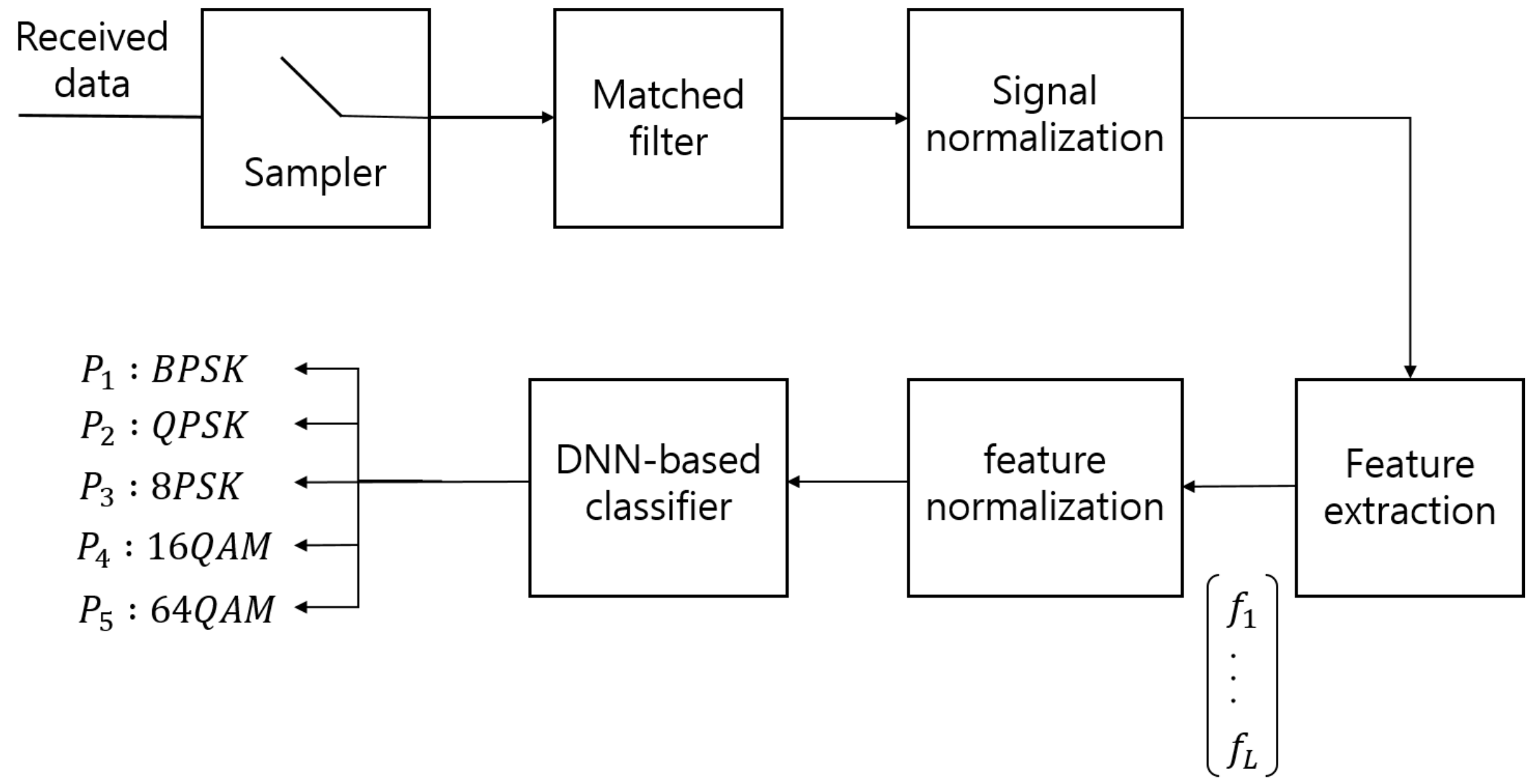
Figure 1 depicts the structure of the proposed DNN-AMC method (DNN-AMC). The received base-band signal samples are obtained by the matched filter followed by the $1/T$ rate-sampler. Then, the feature extractor is applied to convert the base-band signal samples into the L-dimensional feature vector $\overline{f}={[f_1,\dots ,f_L]}^T$. After normalization of the feature vector, the DNN is applied to produce the final classification result in the form of probability that the given modulation class is used. The proposed system goes through two steps: (1) training stage and (2) test stage. In training stage, we generate the M feature vectors ${\overline{f}}^{\left(1\right)},\dots ,{\overline{f}}^{\left(M\right)}$ from the received data samples and optimize the weights of the DNN using them. In test stage, the trained DNN system is applied to the received data samples collected independently from the training data set for evaluation.

4.1. DNN Structure

First, we scale the received signal samples such that they have zero mean and unit variance and calculate the feature vector ${[f_1,\dots ,f_L]}^T$ from them. Then, we normalize the feature vector as

$$\begin{array}{c}\hfill f_i^{\prime }=\frac{(f_i-{\mu }_i)}{{\sigma }_i}.\end{array}$$

(12)

Note that ${\mu }_i$ and ${\sigma }_i$ are obtained from

$$\begin{array}{cc}\hfill {\mu }_i& =\frac{1}{M}\sum _{k=1}^M{f}_i^{\left(k\right)}\hfill \end{array}$$

(13)

$$\begin{array}{cc}\hfill {\sigma }_i& =\sqrt{\frac{1}{M}\sum _{k=1}^M{|f_i^{\left(k\right)}-{\mu }_i|}^2}\hfill \end{array}$$

(14)

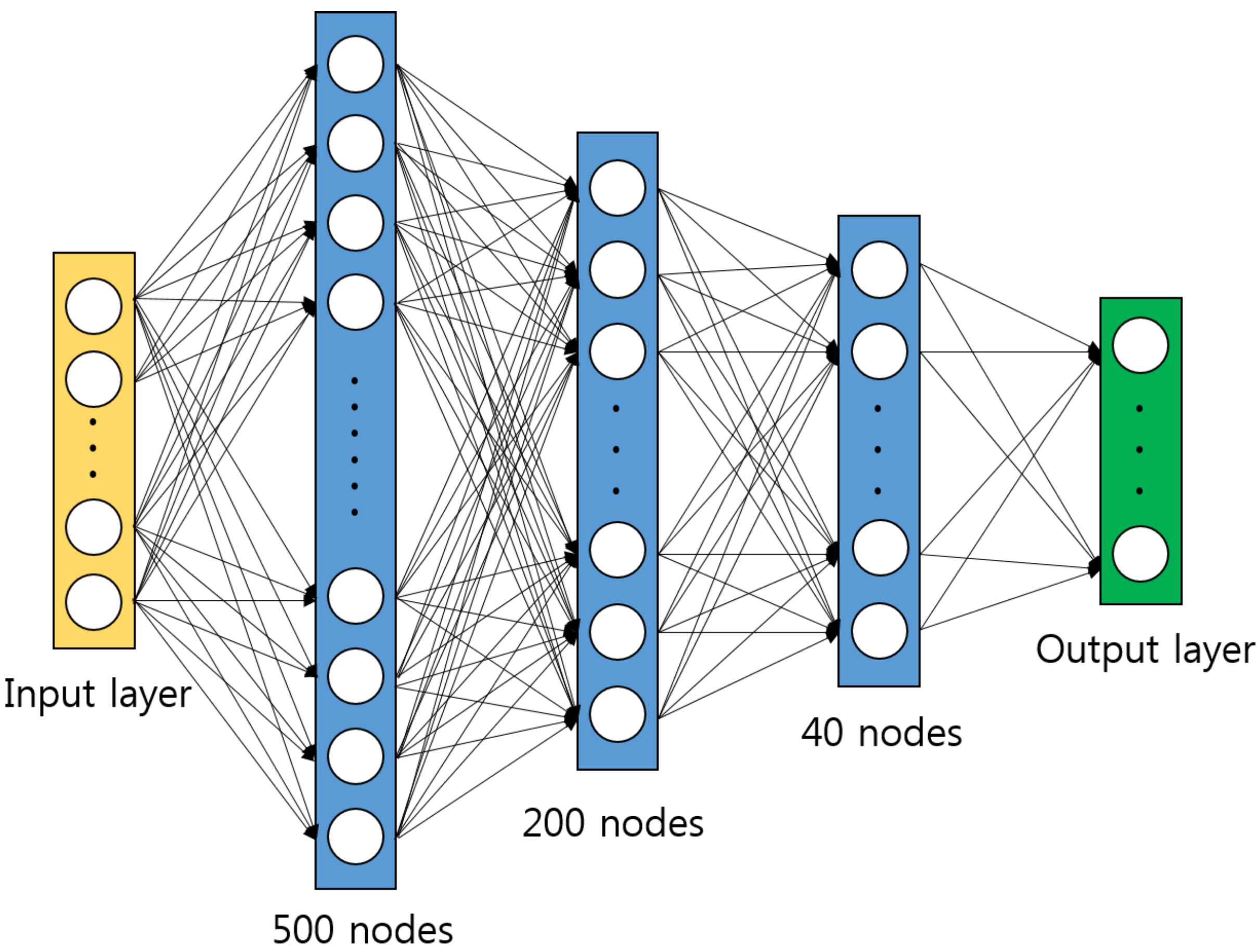
where $f_i^{\left(1\right)},\dots ,f_i^{\left(M\right)}$ are the ith element of the M feature vectors in the training set. Note that in the test phase, we use the fixed value of ${\mu }_i$ and ${\sigma }_i$ that have computed in the training step. The normalization step is nothing but a linear transformation of the features, which makes the feature extraction invariant to any scaling of signal samples. Thus, this normalization step makes the system more robust in real scenarios. The normalized feature vector $[f_1^{\prime },\dots ,f_L^{\prime }]$ is fed into the DNN which consists of the fully connected feedforward network with $Q=4$ hidden layers. Figure 2 depicts the structure of DNN. The rectified linear unit (ReLU) function is used as a nonlinear function [15]. The number of hidden nodes is set to 500, 200, 40, 5 from the input to the output layer, which is determined based on intensive empirical simulations. At the output layer, softmax function is used to produce the probability score associated with each modulation class. That is, the probability score $y_k$ associated with the kth modulation class is given by [21]

$$\begin{array}{c}\hfill y_k=\frac{exp\left(a_k\right)}{{\sum }_{j}exp\left(a_j\right)},\end{array}$$

(15)

where $a_j$ is the activation corresponding to the jth output node. The final classification result is given by choosing the modulation class with the highest probability score.

4.2. Training

As mentioned above, the goal of the training step is to optimize the weights of the DNN using the training data. In the training data set, each feature vector is associated with the class label, which is represented by one hot encoding [21]. We use an appropriate loss function to optimize the weights of the DNN for the given task. For multi-class classification task, negative log-likelihood function is widely used [21]

$$\begin{array}{c}\hfill L=-\sum _{i=1}^{M}log\left(P\left(c^{\left(i\right)}|{[f_1^{\left(i\right)},\dots ,f_L^{\left(i\right)}]}^T,W,b\right)\right)\end{array}$$

(16)

where W and b are the weight matrix and bias vector and $c^{\left(i\right)}$ and ${[f_1^{\left(i\right)},\dots ,f_L^{\left(i\right)}]}^T$ are the class label and the feature vector for the ith training example, respectively. The stochastic gradient descent method with the mini-batch size B is used to minimize the loss function with respect to the weights of DNN. Standard back propagation algorithm is used to obtain the gradient of loss function with respect to the weights at each layer [21]. Note that 20% of training data is not used for the training but for validation. We start with the initial learning rate $ϵ=0.001$, reduce the learning rate by half when the validation error stops to improve, and then, terminate training if validation error converges to fixed value. Note that the training procedure mentioned above is conducted for four scenarios mentioned in Section 3. Note that we generate the training set for Scenario 4 using the randomly sampled channel parameters in order to consider the scenario where the channel parameters are not known.

Table 4. Training parameters.

The Number of Data Samples Converted to a Feature Vector $\left(\mathit{P}\right)$	20,000
The Number of Feature Vectors in Training Set $\left(\mathit{M}\right)$	30,000
The Number of Feature Vectors in Validation Set $\left(\mathit{M}\right)$	6000
Initial Learning Rate $\mathit{ϵ}$	$0.001$
Mini-Batch Size $\left(\mathit{B}\right)$	50

summarizes the training setup used in our experiments.

4.3. Test

Once the weights and biases of the DNN are determined in the training step, we apply the trained DNN-AMC to the test data and evaluate the accuracy of the proposed method. We generate 10,000 test feature vectors and count the number of classification errors for performance evaluation.

5. Experiments

In this section, we evaluate the performance of the proposed algorithm through computer simulations.

5.1. Simulation Setup

In simulations, we consider the classification task that selects one of the five modulation classes, BPSK, QPSK, 8PSK, 16QAM, and 64QAM. We use a raised cosine filter with the roll-off factor 0.2. The symbol rate is set to 10,000 sym/s, and the oversampling rate is set to 10. A feature vector is obtained by processing 20,000 samples (corresponding to 2000 symbols over 0.2 s). M = 24,000 feature vectors are used to train the DNN and 6000 feature vectors are used for validation. We use 10,000 test examples (2000 examples per class) to evaluate the classification accuracy. The classification accuracy for the modulation class c is defined by how many feature vectors are correctly classified among all feature vectors labeled by c.

5.2. Simulation Results

We propose two versions of the proposed DNN-AMC method. The first version called DNN-AMC1 uses all 28 features for classification while the second version, DNN-AMC2 $\left(L\right)$ uses the L features selected based on the list in Table 3. We compare the proposed algorithm with the following existing state of the art AMC methods;

• Artificial neural network algorithm 1 (ANN1) [12]: 10 features ($C_{20}$, $C_{21}$, $C_{40}$, $C_{41}$, $C_{42}$, $C_{60}$, $C_{61}$, $C_{62}$, $C_{63}$, $C_{80}$) are used with the feedforward neural network with single hidden layer.
• Artificial neural network algorithm 2 (ANN2) [13]: 6 features ($\beta$, $v_{20}$, ${\sigma }_{aa}$, ${\sigma }_{ap}$, ${\sigma }_{dp}$, the mean of signal magnitude) are used with the feedforward neural network with single hidden layer.
• Support vector machine algorithm (SVM) [10]: 4 feature vectors ($C_{40}$, $C_{41}$, $C_{42}$, $C_{63}$) are used with SVM.
• Hierarchical classification scheme (HCS) [9]: 3 feature vectors ($C_{20}$, $C_{40}$, $C_{42}$) are used with decision tree classifier.

Note that ANN1, ANN2, SVM, and HCS are trained with the same training data set used for the proposed method. The threshold for the HCS scheme is empirically found for fading channels.

We evaluate the performance of the proposed method. For Scenario 1, all AMC schemes considered achieve 100% classification accuracy for Gaussian channel.

Table 5. Classification accuracy of several AMC schemes for Scenario 2.

	BPSK	QPSK	8PSK	16QAM	64QAM
DNN-AMC1	99.98	93.75	97.58	72.16	74.64
DNN-AMC2 (14)	99.98	90.17	95.22	63.61	69.29
ANN1	97.88	86.16	91.75	57.59	61.93
ANN2	99.69	96.14	40.00	57.34	66.09
SVM	81.9	62.70	74.20	25.40	28.60
HCS	19.22	40.10	65.07	31.38	28.27

and

Table 6. Classification accuracy of several AMC schemes for Scenario 3.

	BPSK	QPSK	8PSK	16QAM	64QAM
DNN-AMC1	99.97	90.37	95.66	69.23	70.85
DNN-AMC2 (14)	99.98	86.79	92.22	67.14	67.7
ANN1	96.65	84.10	90.55	56.32	61.71
ANN2	99.90	63.62	33.27	56.1	69.14
SVM	76.3	65.9	74.4	26.4	39.1
HCS	23.37	41.00	77.71	25.55	49.6

show the classification accuracy for Scenarios 2 and 3, respectively. For both scenarios, the proposed methods, DNN-AMC1 and DNN-AMC2 achieve the significant performance gain over the other AMC methods. We observe that in fading channels, the performance of the proposed AMC method is slightly degraded for higher doppler frequency but significant performance gain of the proposed method is retained. We also observe that the DNN-AMC2 achieves the performance comparable to the DNN-AMC1 which uses the whole set of features considered. This shows that the DNN appropriately controls the contribution from the features depending on their reliability.

Table 7. Classification accuracy of several AMC schemes for Scenario 4.

	BPSK	QPSK	8PSK	16QAM	64QAM
DNN-AMC1	96.61	78.62	85.42	60.22	66.35
DNN-AMC2 (14)	95.58	76.87	83.94	52.96	64.83
ANN1	92.39	72.24	84.40	42.97	58.82
ANN2	84.62	44.02	50.81	45.57	65.90
SVM	67.26	53.7	58.26	26.86	33.92
HCS	18.04	41.28	50.81	35.09	29.24

shows the classification accuracy when the SNR and doppler frequency are randomly distributed. Due to the uncertainty of channel parameters, the classification accuracy of the AMC algorithms is worse in Scenario 4 as compared to other scenarios. Nevertheless, our method outperforms the other AMC schemes significantly as shown in the Table 7.

6. Conclusions

In this paper, we proposed the DNN-based AMC method which can achieve robust classification performance for fading channels. First, we analyzed a variety of statistical features used to perform AMC based on the information theoretic criterion. From this study, we find the key features that are strong for fading channels. The DNN is applied to classify the modulation class based on the statistical features found in our study. Using the feed-forward neural network with four hidden layers, the proposed method achieved good classification performance even when a number of statistical features are used.

References

- Zhu, Z.; Nandi, A.K. Automatic Modulation Classification: Principles, Algorithms and Applications; John Wiley & Sons: River Street Hoboken, NJ, USA, 2014. [Google Scholar]
- Dobre, O.A.; Abdi, A.; Bar-Ness, Y.; Su, W. Blind modulation classification: A concept whose time has come. In Proceedings of the IEEE/Sarnoff Symposium on Advances in Wired and Wireless Communication, Princeton, NJ, USA, 18–19 April 2005; pp. 223–228. [Google Scholar]
- Hazza, A.M.; Alshebeili, S.; Fahad, A. An overview of feature-based methods for digital modulation classification. In Proceedings of the 1st International Conference on Communications, Signal Processing, and Their Applications, Sharjah, UAE, 12–14 February 2013; pp. 1–6. [Google Scholar]
- Azzouz, E.; Nandi, A.K. Automatic Modulation Recognition of Communication Signals; Springer Science & Business Media: New York, NJ, USA, 2013. [Google Scholar]
- Dobre, O.A.; Abdi, A.; Bar-Ness, Y.; Su, W. The classification of joint analog and digital modulations. In Proceedings of the IEEE Military Communications Conference, Atlantic City, NJ, USA, 17–21 October 2005; pp. 3010–3015. [Google Scholar]
- An, N.; Li, B.; Huang, M. Modulation classification of higher order MQAM signals using mixed-order moments and Fisher criterion. In Proceedings of the 2nd International Conference on Computer and Automation Engineering, Singapore, 26–28 February 2010; pp. 150–153. [Google Scholar]
- Huang, F.; Zhong, Z.; Xu, Y.; Ren, G. Modulation recognition of symbol shaped digital signals. In Proceedings of the International Conference on Communications, Circuits and Systems, Xiamen, China, 25–27 May 2008; pp. 328–332. [Google Scholar]
- Xin, Z.; Ying, W.; Bin, Y. Signal classification method based on support vector machine and high-order cumulants. Wirel. Sens. Netw. 2010, 2, 48. [Google Scholar]
- Swami, A.; Sadler, B.M. Hierarchical digital modulation classification using cumulants. IEEE Trans. Commun. 2000, 48, 416–429. [Google Scholar] [CrossRef]
- Li, P.; Zhang, Z.; Wang, X.; Xu, N.; Xu, Y. Modulation recognition of communication signals based on high order cumulants and support vector machine. J. China Univ. Posts Telecommun. 2012, 19, 61–65. [Google Scholar] [CrossRef]
- Han, G.; Li, J.; Lu, D. Study of modulation recognition based on HOCs and SVM. In Proceedings of the IEEE 59th Vehicular Technology Conference, Milan, Italy, 17–19 May 2004; pp. 898–902. [Google Scholar]
- Popoola, J.J.; van Olst, R. Automatic recognition of analog modulated signals using artificial neural networks. Comput. Technol. Appl. 2013, 2, 29–35. [Google Scholar]
- Popoola, J.J.; van Olst, R. Effect of training algorithms on performance of a developed automatic modulation classification using artificial neural network. In Proceedings of the IEEE AFRICON, Pointe-Aux-Piments, Mauritius, 9–12 September 2013; pp. 1–6. [Google Scholar]
- Xi, S.; Wu, H.C. Robust automatic modulation classification using cumulant features in the presence of fading channels. In Proceedings of the IEEE Wireless Communications and Network Conference, Las Vegas, NV, USA, 3–6 April 2006; pp. 2094–2099. [Google Scholar]
- LeCun, Y.; Bengio, Y.; Hinton, G. Deep learning. Nature 2015, 521, 436–444. [Google Scholar] [CrossRef] [PubMed]
- Goldsmith, A. Wireless Communications; Cambridge University Press: Cambridge, UK, 2005. [Google Scholar]
- Tse, D.; Viswanath, P. Fundamentals of Wireless Communications; Cambridge University Press: Cambridge, UK, 2005. [Google Scholar]
- Orlic, V.D.; Dukic, M.L. Automatic modulation classification: Sixth-order cumulant features as a solution for real-world challenges. In Proceedings of the 20th Telecommunications Forum, Belgrade, Serbia, 20–22 November 2012; pp. 392–399. [Google Scholar]
- Guyon, I.; Elisseeff, A. An introduction to variable and feature selection. J. Mach. Learn. Res. 2003, 3, 1157–1182. [Google Scholar]
- Peng, H.; Long, F.; Ding, C. Feature selection based on mutual information criteria of max-dependency, max-relevance, and min-redundancy. IEEE Trans. Pattern Anal. Mach. Intell. 2005, 27, 1226–1238. [Google Scholar] [CrossRef] [PubMed]
- Bishop, C.M. Pattern Recognition and Machine Learning; Springer: New York, NY, USA, 2009. [Google Scholar]
Figure 1.
The structure of the proposed AMC system.
Figure 2.
The structure of deep neural network (DNN) architecture.