Physical Universality, State-Dependent Dynamical Laws and Open-Ended Novelty


1
Beyond Center for Fundamental Concepts in Science, Arizona State University, Tempe, AZ 85287, USA
2
Department of Physics, Arizona State University, Tempe, AZ 85287, USA
3
Algorithmic Nature Group, Laboratoire de Recherche Scientifique (LABORES) for the Natural and Digital Sciences, 75006 Paris, France
4
School of Earth and Space Exploration, Arizona State University, Tempe, AZ 85287, USA
5
ASU-SFI Center for Biosocial Complex Systems, Arizona State University, Tempe, AZ 85287, USA
6
Blue Marble Space Institute of Science, Seattle, WA 98154, USA
*
Author to whom correspondence should be addressed.
Entropy 2017, 19(9), 461; https://doi.org/10.3390/e19090461
Submission received: 27 July 2017
/
Revised: 22 August 2017
/
Accepted: 23 August 2017
/
Published: 1 September 2017
(This article belongs to the Special Issue Entropy, Time and Evolution)
Abstract
:A major conceptual step forward in understanding the logical architecture of living systems was advanced by von Neumann with his universal constructor, a physical device capable of self-reproduction. A necessary condition for a universal constructor to exist is that the laws of physics permit physical universality, such that any transformation (consistent with the laws of physics and availability of resources) can be caused to occur. While physical universality has been demonstrated in simple cellular automata models, so far these have not displayed a requisite feature of life—namely open-ended evolution—the explanation of which was also a prime motivator in von Neumann’s formulation of a universal constructor. Current examples of physical universality rely on reversible dynamical laws, whereas it is well-known that living processes are dissipative. Here we show that physical universality and open-ended dynamics should both be possible in irreversible dynamical systems if one entertains the possibility of state-dependent laws. We demonstrate with simple toy models how the accessibility of state space can yield open-ended trajectories, defined as trajectories that do not repeat within the expected Poincaré recurrence time and are not reproducible by an isolated system. We discuss implications for physical universality, or an approximation to it, as a foundational framework for developing a physics for life.
1. Introduction
Schrödinger’s seminal 1943 lectures titled “What is life?” [1] laid out a compelling challenge for physicists to explain the properties of living matter from what we know of physics. Based on logic and consideration of constraints imposed by physical laws (e.g., the second law of thermodynamics) Schrödinger was able to accurately predict that the genetic material should be “an aperiodic crystal” i.e., a stable molecule with a non-repeating pattern, which was only later discovered to be DNA. He conceded towards the end of his book that “living matter while not eluding the ‘laws of physics’ as established up to date, is likely to involve ‘other laws of physics’ hitherto unknown” (arriving at this conclusion was in fact a motivator for Schrödinger to write the book in the first place). The challenge, as Schrödinger saw it, was to understand the function of the genetic material in purely physical terms: that is, how matter can both direct the transformations necessary for development of an organism and
also how it can reliably transmit the capacity to perform those same transformations to future states of an organism (exhibiting stability) and its progeny (through self-reproduction).
Around the same time, von Neumann set out to determine the architecture of natural and artificial self-reproducing automata based again on logic combined with consideration of simple physical constraints (such as the finiteness of available resources and available time) [2]. He showed that self-reproduction is logically possible for a constructor, which he defined as a machine capable of being programed to perform physical transformations, including transforming available resources to produce a copy of itself. To guarantee that self-reproduction is possible, von Neumann hypothesized the existence of a universal constructor: a physical system capable of being programmed to perform any possible physical transformation. If universal construction is possible under a given set of dynamical laws, self-reproduction must necessarily also be possible (being just one class of physical transformations). One motivation for taking this conceptual leap is to explain how biological processes could be open-ended: life on Earth is characterized by continual adaptation and innovation, giving rise to an apparent open-ended increase in the complexity of the biosphere over its several billion year history. In addition to the more obvious universal limitations including the finiteness of resources and constraints imposed by the laws of physics, a self-reproducing constructor is limited in its ability to reproduce by two additional constraints: the physical transformations it can perform and the number of programs containing its specification. This includes specifications of constructors close enough to the original to permit semantic closure under mutation, see e.g., [3] for discussion. For a universal constructor only the latter is a limiting factor, since it can perform any physical transformation (viz reading any possible program). Therefore, at least in principle, a universal constructor should have the maximal capacity of any physical device for open-ended evolution, with important implications for understanding biological evolution [4]. By focusing on the logical structure of a such a system, von Neumann was able to solve part of the problem posed by Schrödinger. However, he stopped short of solving the harder problem of how such a device could follow from physical principles (this harder problem was recently advanced byMarletto in [5] within the formalism of Constructor theory).
We do not know whether a universal constructor is itself physically possible in our universe [6], or if such an entity is necessary for open-ended evolution in a dynamical system (only that it is sufficient). One necessary condition for a universal constructor to be possible is physical universality, defined as the property that any possible physical transformation can be performed on a given system, provided sufficient resources are available to do so and subject to the requirement the transformation(s) do(es) not violate any laws of physics (e.g., one could not build a perpetual motion machine even with a universal constructor). The key distinction between physical universality and the related, more widely discussed concept of computational universality, is that for the former computation (more aptly construction) is performed directly on the physical system, such that transformations are on states rather than on emergent patterns. If physical universality can be cast as a principle of nature it could provide a promising candidate framework for arriving at the “other laws” Schrödinger hoped might one day be uncovered. It would also likely provide new insights into the structure of physical reality, e.g., as is being pursued in Constructor theory, which takes as its foundation describing what transformations are possible and why [7]. A formal definition of physical universality was proposed by Janzig, where a dynamical system (as described by a Hamiltonian or cellular automaton) is physically universal if any transformation whatsoever can be implemented on any finite region [8], given sufficient resources to do so. So far, three examples of physical universality have been proven in cellular automata (CA), which satisfy Janzing’s definition: two classical [9,10] and one quantum [11]. However, the proof of physically universality in each of these cases involves evolving the system to an inactive state, implying that the dynamics cannot be open-ended. Whether or not physical universality permits open-ended dynamics (such that a universal constructor, if instantiated, could exhibit open-ended evolution) remains an important open problem.
In this paper, we focus on the more fundamental concept of physical universality, as a necessary prerequisite condition on the physics underlying von Neumann’s universal constructor architecture (UCA). We address whether a notion of physical universality exists that is compatible with open-ended evolution, and under what circumstances a system could be both physically universal and open-ended. Although our work is motivated by evolution in the biological sense, the term “evolution” intended here is broader and refers to the capacity for dynamical systems to change in time: it therefore applies both to prebiotic systems and the subsequent architectures of physical systems that have supported various stages of biological evolution. That is, we aim to address the physical principles that permit open-ended novelty to be possible in the first place. To do so, we investigate a new variant of cellular automata, introduced by us in [12,13] in which the dynamics are permitted to be state-dependent. We show how state-dependent dynamics can enable both physical universality and open-ended evolution at the same time, by increasing the number of transformations possible in a deterministic system. In what follows, we first review the relevant properties of known physically universal CA, and explain the key differences in the model proposed herein. We then implement simple examples with state-dependent architecture to demonstrate properties of the underlying state-transition diagram which could enable physical universality and open-ended evolution. A limitation of Janzig’s definition as applied to biosystems is that it necessitates dynamical laws that are reversible (such that it is possible to run them backwards in time), otherwise information in the initial state would be lost and could not be recovered by running the dynamics in reverse (that is, not every state would be accessible to the dynamics). We introduce a relaxed definition of physical universality, local physical universality, that applies to subsets of transformations, rather than all possible transformations. We show reversibility is necessary for physical universality (or its approximation) only if the dynamical laws do not evolve in time, permitting the possibility of physical universality in irreversible dynamical systems. Since dissipation is ubiquitous in biology, and effective descriptions of living systems are in-general state-dependent, our model provides a more appropriate starting point for understanding physical universality as it might underlie living processes, as we discuss in the conclusion.
2. Physical Universality and Local Physical Universality
CA are widely studied due to their simplicity and their ability to capture two key features of many real physical systems: they evolve according to a local, uniform deterministic rule, and can exhibit rich emergent behavior even from very simple rules (see e.g., [14,15,16,17,18,19,20,21]). The physical laws governing our universe may not be completely deterministic (for example, under collapse interpretations of quantum theory) nor is reality necessarily discrete. However, by demonstrating a proof-of-principle for the more conservative and conceptually easier case of discrete deterministic systems it can be expected that at least some aspects will be sufficiently general to apply to physical laws as they might describe our real universe, under relaxed assumptions. For example, several CA are known to include patterns supporting computational universality (e.g., are Turing machines). Two well-known examples are Conway’s Game of Life [22] and Elementary Cellular Automata (ECA) rule 110 [23]. In these examples, an input tape (the CA’s initial state) must be formatted and typically consists of emergent spatiotemporal patterns such as gliders, particles, spaceships etc. A limitation of this kind of universality is that it requires a programmer, or agent, to decide what patterns are doing the computation and how they will do it. Janzing’s introduction of physical universality removes the agency in specifying computational degrees of freedom by introducing a concept of computation that can be performed arbitrarily on all patterns and not just the carefully constructed ones. A CA is physically universal if it can implement any transformation whatsoever on any finite region of the CA’s state in finite time. Of note, von Neumann’s original CA model of a universal constructor was not physically universal by Janzig’s definition, but instead operated on patterns as in models of computational universality (first implemented by Nobili and Pesavento [24]).
Janzing’s interest in developing a framework for physical universality was to provide the foundations for a physical model of control where the boundary between a controller and the physical system it controls can be shifted, and there is no difference in the physics of the controlling and controlled systems. His definition specifies two regions of the CA: a finite region (the controlled system) and the complement of the region (the surrounding cells, forming a “controller”, which is a potentially infinite resource). With this setup, physical universality is possible when any transformation of the controlled region can be implemented through the autonomous evolution of the system after the surrounding controller has been initialized in an appropriate way. (Roughly, the controlled and controller regions could be considered as data and program, respectively). More formally (adopting the slightly modified but equivalent definition of Schaeffer [9], and following his notation), we can define a CA where each cell has a state in the finite set , with cells positioned at integer points in d dimensions (in this work we focus on explicit examples of Elementary Cellular Automata with , but consider the most general definition here). Defining as the set of all cells, for a set the compliment of X in is (the set of cells that do not belong to X in ). A configuration of a subset of cells is a map assigning each cell in X a state in , such that denotes the set of all possible configurations of X. The transformation of a configuration into another configuration after one time-step is denoted . With this notation, physical universality is defined as:
Definition 1. Physical universality.
Let be finite sets. Let f be an arbitrary function that maps , then a configuration implements the transformation f in time T if for any configuration there exists a configuration such that , where ⊕ is the direct sum.
A cellular automaton is physically universal if for any finite input region , output region , and transformation f, there exists a configuration ϕ of such that ϕ implements f in finite time.
In other words, if a configuration of the compliment region (the controller) can implement any transformation f on an input x in the region of interest, evolving it in a finite number T of steps to a configuration , then the CA is physically universal.
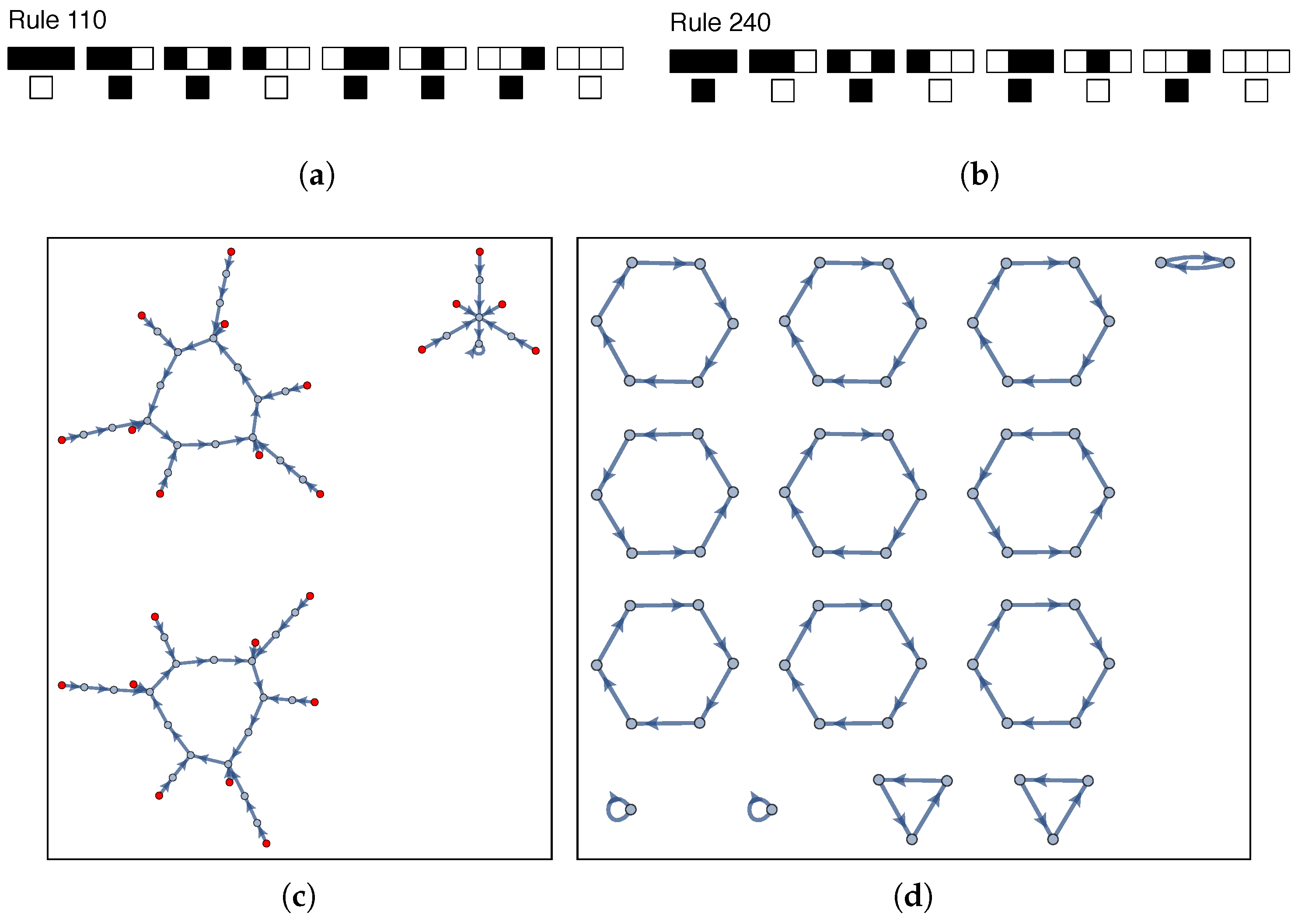
Physical universality as defined by Janzing places strict constraints on the properties of CA (or the laws of physics in the real universe). One troublesome aspect is the controller, which cannot be an emergent property of the dynamics in Janzig’s formulation. Instead the controller is merely defined away as ‘the rest of the universe’ and can, in essence, be reduce to the laws of physics operating on an appropriate initial state, which is not explanatory of life (see e.g., [25] for related discussion). Assuming fixed dynamical laws, one necessary (but not sufficient) condition for physical universality is reversible laws. In CA reversibility corresponds to rules that yield bijective state-transition maps from : every state maps to exactly one other state, such that there are no “Garden of Eden” states (states that can only be an initial state). If this were not so, the CA could evolve to a configuration where no output is possible (halting the computation). Below we focus on Elementary Cellular Automata (ECA, described in Section 5) as the rule space for our state-dependent CA. Two examples of the state-transition diagrams for an irreversible and a reversible ECA rule for rules 110 and 240 (using Wolfram’s numbering scheme [20]), respectively, are shown in Figure 1 for six-bit CA () with periodic boundaries (It should be noted that for arbitrary CA specified on a Moore neighborhood, where each cell is updated based on its current state and the state of its nearest neighbors, it is in general undecidable whether a CA is reversible [26]). Computationally universal CA, such as rule 110, are often not reversible (an exception is Margolus’s CA model of the billiard ball model of computation from Fredkin and Toffoli [21]). Thus, even though a computationally universal CA may be able to compute any possible computable function (is computationally universal) it may not be capable of producing any possible output of cells (required for physical universality). Universal computation and universal construction are discussed by Deutsch as two separate possible principles of nature (the computability and constructibility of nature, respectively), both of which remain to be proven, see [6].
Since the laws of physics are normally microscopically reversible, physical universality is at first pass compatible with known physics. However, in our universe there are cases where reversibility does not precisely hold, for example in charge, parity symmetry (CP) violation in weak interactions. More relevant to life is the fact that, in microscopic and macroscopic physical systems, the effective laws of physics are very often irreversible, on account of the fact that they are dissipative. Irreversibility is likely essential to emergent properties in biological systems, for example, it is a requirement of formal definitions of causal emergence [27]. Since the emergence of an arrow of time is essential to life, the question arises: can a principle of physical universality be made compatible with a universe where irreversibility exists (if not microscopically at least as an emergent property)?
The requirement of physical universality that every transformation be possible in a finite region is too stringent for us to make progress. However, we can consider a weaker situation in which there exist subset(s) of configurations with the property of inter-accessibility (that any transformation is possible within a given subset). We introduce the concept of local physical universality for this weaker case, using a definition, which follows from the definition of physical universality:
Definition 2. DLocal Physical Universality.
Let be finite sets. Let g be an arbitrary function that maps , where and . Then, a configuration implements the transformation g in time T if for any configuration there exists a configuration such that .
A cellular automaton is locally physically universal if for any finite input region , output region and transformation g, there exists a configuration of ϕ on such that ϕ implements g in finite time.
That is, a system is locally physically universal if for any finite region all transformations are possible within a given subset of configurations . Locality here is meant to indicate the connectivity of the underlying state-transition map: in a locally physically universal cellular automata the state-transition map will contain connected components where there exists a directed path between all ordered pairs of states, defining a local neighborhood in configuration space where one can traverse a path from any state to any other state. In this sense the closed loops in the state-transition diagram of rule 240 in Figure 1 are locally physically universal. All reversible fixed dynamical laws exhibit local physical universality. In the limit , local physical universality is trivial (arbitrarily small subsets of states can be locally physically universal). In the limit local physical universality converges to a principle of physical universality that holds over all transformations among all configurations. The utility of this definition is that it permits discussion of varying degrees of physical universality, and therefore the possibility for the universality of a system to change in time (e.g., as has been the case in the transition from prebiotic to biological evolution).
Schaeffer was the first to introduce an example of a physically universal CA satisfying Definition 1. Schaeffer’s CA has a local update rule that operates on a 2-by-2 block (Margolus neighborhood) in . The CA behaves like a diffusive gas: time evolution of a bounded region results in particles diffusing outside of that region, such that a finite region will converge to an inactive state for long times. The advantage of this is that it permits all information about what happens within a box to be intercepted as particles diffuse outside it, allowing reconstruction of what happens inside the box. Schaeffer leveraged this property to prove any possible transformation of particles inside a box can be programed (physical universality is possible) by suitably preparing the state of the system outside the box. Subsequently, Schaeffer demonstrated a quantum version [9] and Salo and Törma [10] demonstrated a one-dimensional version. Proof of physical universality for these examples follows similar logic (see [11] for discussion) and relies on tracking states backwards in time from dynamics that converge to an inactive state. Since the physically universal region in these CA terminates in a quiescent state, the physically universal region cannot exhibit another key property of life: open-ended dynamics.
3. State-Dependent Dynamical Systems
We aim to show that physical universality is possible in state-dependent CA, and that for these systems open-ended evolution is also possible. State-dependent dynamical systems are ones where update rules are not fixed as a function of time, but rather change as a function of the current state of the system (for example, in biological systems when the level of gene expression in turn dictates the turning on and off of genes), such that laws and states co-evolve [13,28,29]. State-dependent dynamics are frequently discussed as a hallmark feature of life [30,31], and provide one possible conceptual framework for understanding emergent properties in living systems in terms of physical principles [32]. In a state-dependent dynamical system, information encoded in the states determines what transformations can occur [33]. State-dependent dynamical systems therefore provide an intriguing framework for understanding physical universality in the case where some transformations are enabled by the particular information-processing architecture of physical systems.
In Adams et al. we showed that the co-evolution of laws and states permits greater range in the dynamical trajectories accessible to a system than what is possible with a fixed dynamical rule [12]. The number of paths through configuration space accessible to a system increases, since information encoded in the states enables transitions between different trajectories allowed by fixed dynamic laws (e.g., between the disconnected components in Figure 1) [13]. The minimal requirement for physical universality is that all states are a possible output of the dynamics, that is that the number of possible outputs is equivalent to the number of possible inputs of the dynamics, yielding the requirement of a bijective map for fixed rules. Because many different rules can govern transitions in a state-dependent system, the requirement is relaxed to dynamics that are surjective. This relaxed condition makes it possible, at least in principle, for a system with state-dependent rules to exhibit physical universality, even if its dynamics are irreversible (a surjective map is in general not reversible since it can be many-to-one or many-to-many or one-to-many).
We postulate physical universality is possible with state-dependent rules and that it can occur even in cases with irreversibility, so long as the state-transition diagram is surjective. To explore this we adapt a state-dependent cellular automaton introduced by us in [12] and show examples of systems that are locally physically universal, excluding states that contain no information (all-“0” and all-“1” states). Our original model included two interacting CA: an “organism CA” and “environment CA”. To bring this abstract model in closer contact with the structure of a physical device necessary to implement such dynamics, we here recast the organism CA and environment CA as the system to be controlled and a resource (program), respectively. Our formulation does not map directly to the universal constructor architecture (UCA) proposed by von Neumann, as we are focused on the related but distinct problem of physical universality and, as noted in the introduction, do not address the problem of biological evolution in our model (instead focusing on the prerequisite conditions for physical universality).
In von Neumann’s formulation, self-reproduction of a constructor requires a physical device to store a program, which specifies the instructions for the assembly of a new copy of the constructor. Since no physical device can store the infinite amount of information necessary to specify a constructor’s progeny, and all its subsequent descendants ad infinitum (pending available resources) a self-reproducing constructor must necessarily carry a control system—termed a supervisory unit—telling the constructor when to produce a copy of its program (or more precisely, when to assemble a duplicate of the physical system storing the program) versus when to read it. That is, the supervisory unit must decide when the instruction set is to be treated as software to be read and when it is merely hardware to be blindly copied. Drawing an analogy with this architecture, the controller (analogous to the rule of the supervisory unit) in our model is the function that specifies the interaction between the system and resource, the system plays the role of the constructor and the resource plays the role of the program or tape.
A schematic of our system is shown in Figure 2a and a CA implementation in Figure 2b. Both the system and resource implement ECA rules and may therefore be considered to implement the same “physics”, e.g., the same set of local rules. The distinction between the two emerges due to their interaction: the system’s update rule is state-dependent and changes in time as a function of the system’s state and the state of the resource CA (under direction of the meta-rule). As a concrete example of when such a setup might occur, one can consider a chemical reaction where it is desired for a particular chemical species to be transformed into another. The controller in this case could be catalyst (an example of a constructor discussed in [7]) and the resource is other substrates necessary for the reaction. Different transformations can be performed on the same substrate, if in contact with different catalysts and/or different resources. We additionally note the architecture we impose is consistent with other physical models of information dynamics: for example, modern incarnations of Maxwell’s demon are structured such that a device is coupled to an external tape or program (see e.g., [34]). In these models, the tape and device are not in general constrained to obey the same dynamical laws, but the thermodynamics are well defined within the context of the model (see [35] for example where demon and system obey the same dynamics). Here we do not address the thermodynamics of our devices, but within the rule structure of CA we do enforce that system and resource obey the same set of physical laws.
Janzing required that the controller and controlled system have the same physics, and that the boundary between the two systems be arbitrary. Physical universality can be demonstrated for a finite region (the controlled system) by suitably programming the initial state of its complement. The structure of our CA is different in two key aspects. The first is that the role of the controller is played by a “metarule” that dictates the interaction between the two interacting subsystem CAs (Note that this metarule should be constrained to obey the same laws of physics as the CA, to conform to Janzing’s definition of physical universality). We additionally define hard boundaries around the system and the resource, noting that boundaries are often discussed a fundamental to life (see e.g., [36]). Boundaries are implemented by isolating the states of each CA with periodic boundary conditions. However, as in Janzing’s case the size of the region to be programmed (the system) can be specified arbitrarily, and the only requirement is that the region be specified prior to determining if it is physically universal. Our motivation for implementing the hard boundary is to focus on the role of state-dependent rules in enabling physical universality and open-ended evolution: we construct our system such that the only external interaction is through the controller’s regulation of the update rule. The controller does not control the boundary of the states in our case. Because our system has closed boundary conditions, configurations containing no information—the all-“0” or all-“1” states—are cut-off from the rest of configuration space: once a system lands in one of these states it cannot escape as there is no ECA rule that can transform states outside the set of two homogeneous states. Therefore it is not possible for our system to display true physical universality; nonetheless we do show that local physical universality is possible among all other states. We expect that in cases where our devices are permitted to have boundaries that interact with other systems, physical universality will be readily possible, as in other examples of physical universality where open boundaries are necessary (such that information can flow through the boundary).
4. Open-Ended Evolution
In [12] we proposed formal definitions of unbounded evolution and innovation applicable to any instance of a dynamical system U that can be decomposed into two interacting subsystems and (such that ). These definitions are constructed to satisfy two of the four criterion for a system capable of open-ended innovation as presented by [37], including: (1) on-going innovation and generation of novelty; (2) unbounded evolution; (3) on-going production of complexity; (4) a defining feature of life. Based criteria (1) and (2) we defined a minimal criterion for open-ended evolution: a region is open-ended if it satisfies the requirements for unbounded evolution and innovation [12], defined below. As we showed in [12] the other two criteria emerge naturally as a consequence of the state-dependent framework.
Unbounded evolution (UE) can be formalized by comparing the dynamics of a system to the expected Poincaré recurrence time . For any finite, deterministic dynamical system, the Poincaré recurrence time provides a natural bound on its dynamics and is defined as the timescale at which the system’s dynamics should repeat if it were isolated. Unbounded evolution is therefore minimally defined as occurring only in cases where the recurrence time locally exceeds this bound.
Definition 3.
Unbounded evolution (UE): A system U composed of at least two interacting subsystems interacting according to an arbitrary function , exhibits unbounded evolution if there exists a recurrence time such that the state trajectory for is non-repeating for and is the Poincaré recurrence time of a finite region , where is an isolated equivalent of without the interaction with under .
That is, a system exhibits UE if its recurrence time is greater than the Poincaré recurrence time expected for an equivalent isolated system, denoted . By this definition, a system can exhibit UE if and only if it is interacting with an external system. In [12] we included rule trajectories non-repeating in in our definition of UE. For simplicity, since we only consider state-trajectories in the present work we do not include rule trajectories in the definition here. Implementing this definition necessarily depends on knowledge of counterfactual histories of isolated systems (e.g., for systems implementing ECA rules, these counterfactual histories are of ECA executed with no external interaction, see [12]). We additionally define innovation relative to counterfactual histories of isolated systems as:
Definition 4.
Innovation (INN): A system U composed of at least two interacting subsystems interacting according to an arbitrary function , exhibits innovation if there exists a recurrence time such that the state trajectory for is not contained in the set of all possible state-trajectories for a finite region in isolation.
That is, a subsystem exhibits innovation if and only if its dynamics are not contained within the set of all possible trajectories of equivalent isolated systems. For the case of CA, this implies that a finite region is innovative if its state trajectory cannot be reproduced by any static-rule CA with the same width w under the same rule space (here constrained to the set of ECA rules). We note that the Poincaré recurrence time for most real physical systems (including life) is much longer than the age of the universe: the utility of our definition is that it is precise and permits asking quantifiable questions about the kinds of dynamical systems that could, at least in principle, exceed this bound.
A motivation for including both Definitions 3 and 4 is that they encompass intuitive notions of “on-going production of novelty” (INN) and “unbounded evolution” (UE), both of which are considered important hallmarks of open-ended evolution (OEE) as outlined in [37]. The combination of both definitions excludes cases that continually produce complexity but are intuitively not open-ended, such as trajectories produced by ECA Rule 30, which is known to generate complex dynamics that continually create novel patterns under open-boundary conditions [20]. In this case, it is the open boundaries which generate the continual novelty rather than an internal mechanism of Rule 30. Since we aim to understand the intrinsic mechanisms that might drive OEE in real, finite dynamical systems, we require that both definitions are satisfied for a dynamical system to qualify as being capable of non-trivial OEE.
Our goal here is to determine if a subsystem S can be open-ended and physically universal, or minimally at least open-ended and locally physically universal. We next introduce a more detailed description of our setup and toy model implementation and show how the capacity of state-dependent CA to satisfy the formal requirements for OEE depends on the topology of their underlying state transition diagram, focusing on whether there are regions of configuration space that are locally physically universal.
5. Methodology
Following our setup in [12], we study a CA composed of two coupled subsystems, each using local update rules drawn from the set of Elementary Cellular Automata (ECA). ECA have , with nearest neighbor update rules that operate on the alphabet [20]. They are popular models for studying the behavioral complexity of discrete dynamical systems. A schematic of our setup is shown in Figure 2a and a CA implementation in Figure 2b. The model includes the following parts:
Resource: The resource is a CA of finite width w evolving according to constant function , where and is a subset of ECA rules (e.g., is an ECA, sets used in this study are described below).
System: The system is a CA of finite width w evolving according a state-dependent map , where and and are the configuration of and at time t, respectively, and is the rule implemented by the system at time t. As with the resource and is a subset of ECA rules (here the system implements an update rule drawn from the same set of rules governing the resource to ensure both obey the same “laws”).
Controller: In the definition of the system, the controller is an arbitrary function mapping the rule of the system at time t to that at , such that the rules of evolve in time in addition to the configurations. We regard the ‘metarule’ as the controller for the interaction between and . For the results presented here is defined as follows:
where the Round function chooses the nearest upper rule r in the set of , w is the width of each CA, and and are the configuration of and as before, respectively (these are converted from binary representation to decimal). If the expression evaluates to a value >255 (outside the index range of ECA rules), then the evaluated value is depreciated by 255.
We studied this setup using a variety of interaction rules , with similar qualitative results achieved in each case. The only critical constraint on is that it is be a function of , and , such that the update rule of depends on the previous state of the system and resource. In this way, our setup is somewhat akin to the structure of a Turing machine (or von Neumann’s UCA) where the each step in a computation depends both on the internal state of the machine and the state of the tape (program) being read [38] (that is, our system is self-referential). Because we are interested in the possibility of physical universality and open-ended dynamics in we do not explicitly implement a CA instantiation of here. However, we note to study physical universality (and open-endedness) as an emergent property of the dynamics one would need to explicitly implement with the same sets of laws as and . The emergence of feedback control is one of the most challenging open problems in the origins of life [33,39], the exploration of which in state-dependent CA we leave as a subject of future work.
For the results presented here, both the resource and the system are implemented with periodic boundary conditions and a stationary size w (the width of the CA). As stated above, because we impose periodic boundary conditions, the examples presented cannot represent true physical universality—once an empty configuration (all 0’s or all 1’s) is achieved the system has no ability to generate new behavior and becomes inactive. This is also a constraint on reversible CA in the standard approaches to physical universality, including the examples of Schaeffer and Salo and Törmä [9,10]. It is resolved by assuming the compliment region can be made arbitrarily large, potentially requiring infinite resources. In our setup a similar solution of coupling to an arbitrarily large resource could be implemented, by permitting our system to have open boundaries (rather than periodic) in direct contact with the resource, which could be made arbitrarily large. Since our primary motivation is to isolate how state-dependent rule evolution might enable physical universality and open-ended evolution, we do not include the additional complexity of coupling the state of our system directly to the state of the resource (through a shared boundary), which will be a subject of future work. Exclusive of this constraint we do observe systems able to explore the majority of their state space, providing insights into how adopting a state-dependent framework (where new rules emerge at different scales) might open new paths to understanding the ability of biological systems to explore their configuration space, in turn providing new frameworks for explaining physical universality.
5.1. Classifying ECA Rules by Reversibility
In [12] we considered a scenario where the coupled system had access to any ECA rule for the update function of S. Here, we classify ECA rules by the fraction of all possible inputs they can produce as an output—which may roughly be considered as their irreversibility—and implement state-dependent CA with access to rules that share similar irreversibility. This amounts to merging the state-transition diagrams of CA with similar irreversibility to generate variants of our setup in Figure 2b with different topologies for the underlying state-transition diagram of . This permits constructing state-dependent systems with varying capacity to support the possibility of local physical universality and varying ability to support open-ended evolution. Define and as the set of all possible output and input states, respectively. Then, we define the “degree of irreversibility” of an ECA rule r for a given CA width w as the ratio of the number of unique outputs that rule can produce (given all possible inputs ) to all possible inputs , for a single time step t:
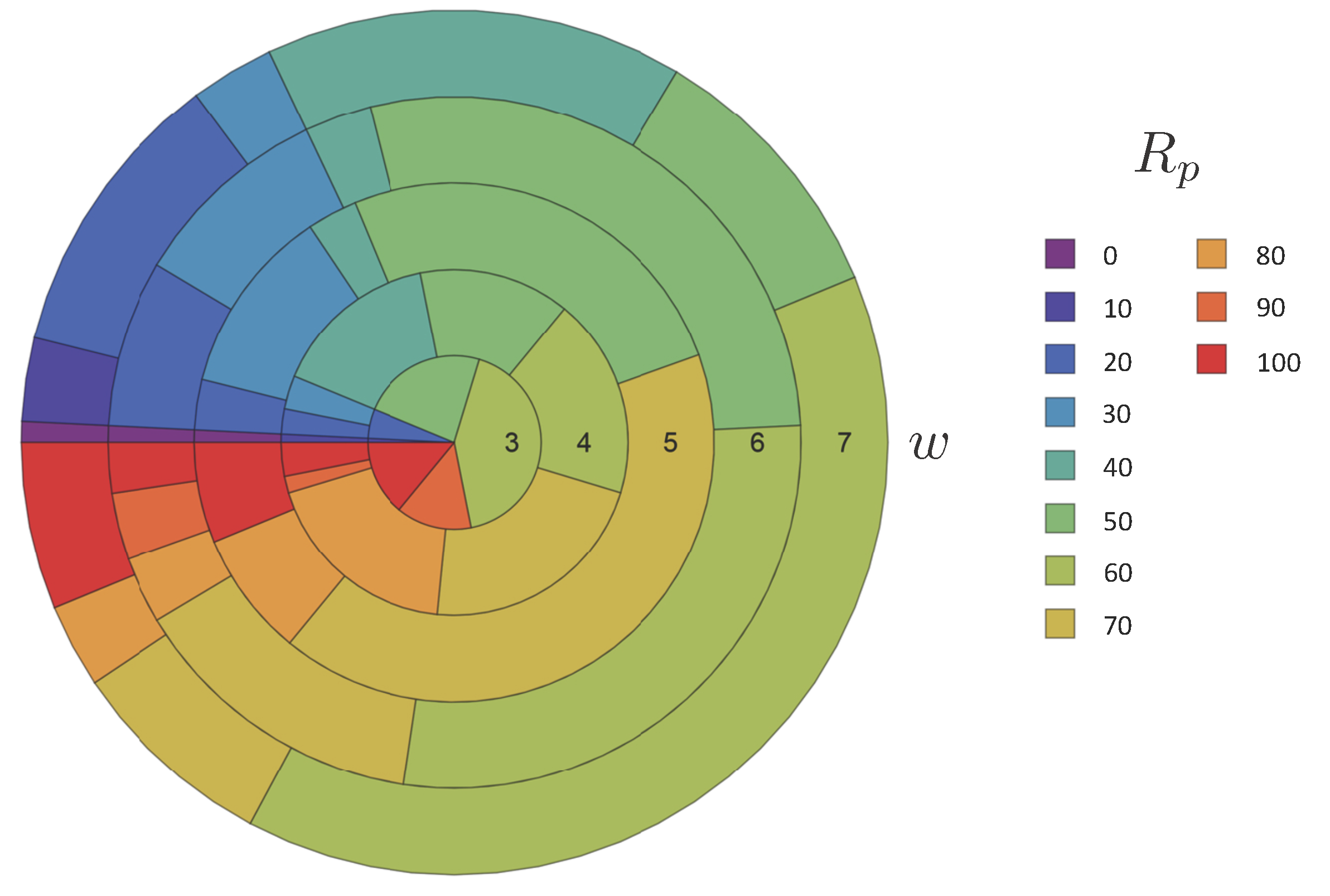
For , a rule is fully reversible, preserving information about its past state(s). For all other values the rule is irreversible, quantified on a sliding scale by how much information the rule destroys about past states. For the system is completely irreversible and looses maximal information (e.g., ECA rules 0 and 255 which map all states to the all-“0” or all-“1” state, respectively). We calculated R for all ECA rules and partitioned the rules by rounding to the nearest , thereby identifying 11 sets for each width. The relative size of each set is plotted in Figure 3 as a function of w.
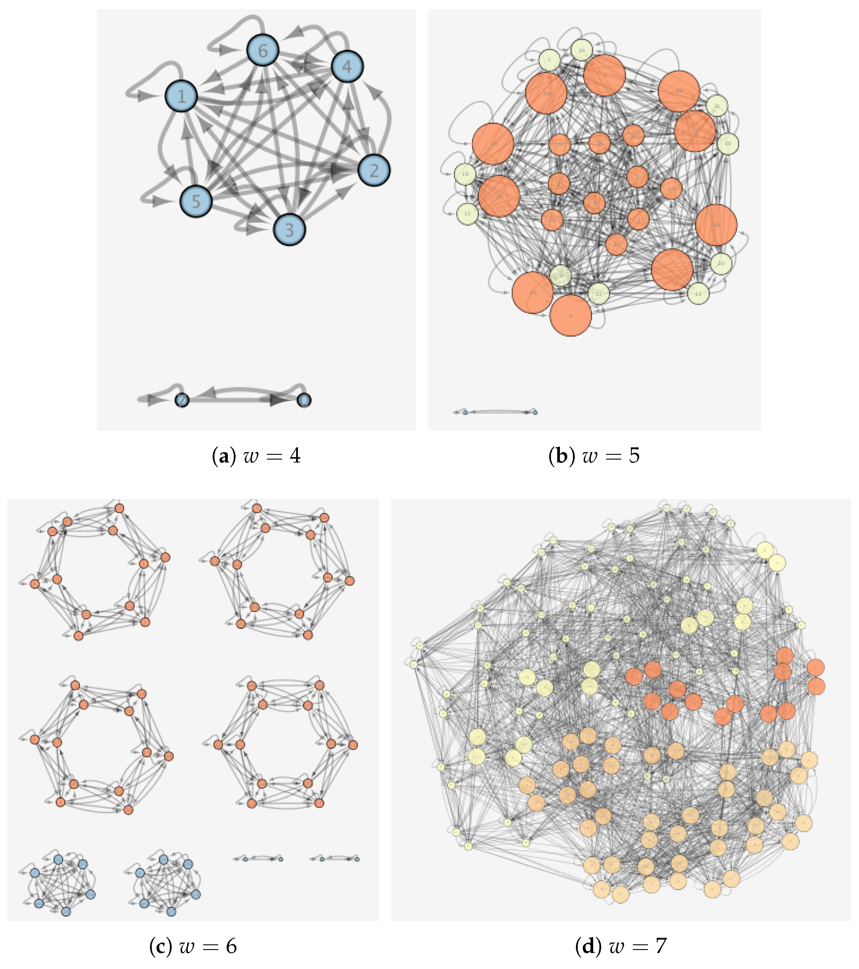
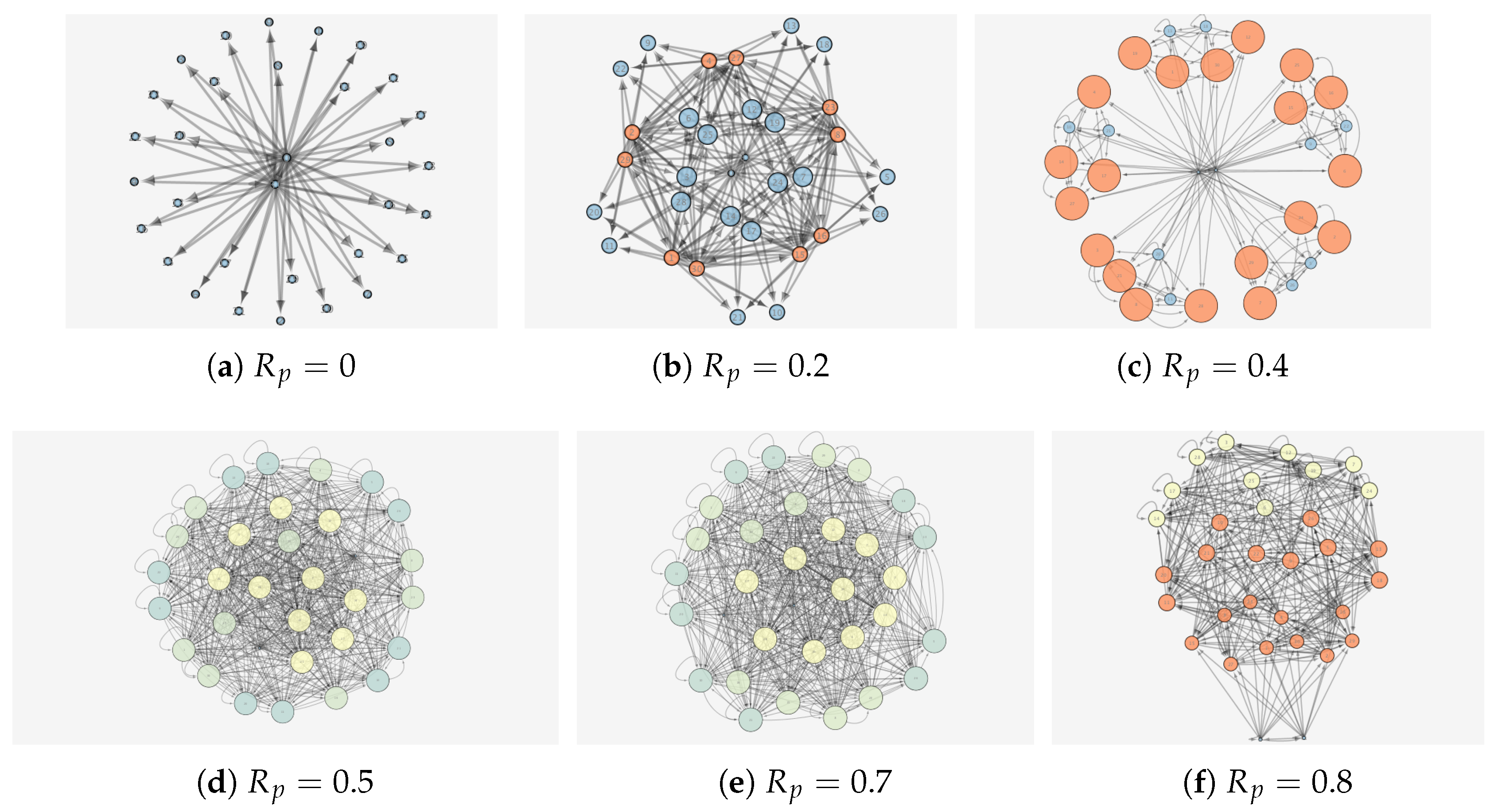
By merging rules within a given reversibility class, we construct state-dependent state-transition diagrams where we can control the accessibility of states. We constructed the composition of all state-transition graphs for a given , which we label as for a given width w. Examples are shown in Figure 4 and Figure 5. In these diagrams, nodes represent CA states and directed edges represents a rule that allows a transition between the connected states. The interaction function and the state of the program (resource) CA together determine the realized trajectories through the state-transition diagram (and are external to this graph). For state-transition diagrams generated from all rules, we know all states are accessible a priori. is therefore a good candidate for studying how (local) physical universality could enable open-ended dynamics. Conversely, for we know almost no states are accessible to the dynamics (and therefore OEE and physical universality are impossible). We expect the likelihood of open-endedness will depend in part on the topology of the state transition diagram (There is also a resource dependence, where the recurrence time of the system in general scales linearly with that of the resource, see [12]). We analyzed the structure of the state-transition diagrams using several common topological measures, including: mean in-degree, the average number of inputs for each state; mean out-degree, the average number of outputs from each state; average shortest path, the average smallest number of transformations (steps) to move between any directed pair of states; and betweeness centrality, the number of shortest paths passing through a given state (shown in Figure 4 and Figure 5). We also determined the number of connected components and the size of the largest connected component, where a connected component is a region of the state-transition diagram where any two states are connected to each other by some (undirected) set of transformations, and which is connected to no additional states in the state-transition diagram. We equate the accessibility of state-space with physical universality if all states in a graph can be reached from any other state, the system is physically universal. If this is only true for a subset of configurations (a connected component) that set is locally physically universal. We next study the dynamics and likelihoods of generating OEE for state-transition diagrams constructed for each class of a given width to determine how accessibility of the state space (topology) constrains or enables open-ended evolution.
6. Results
6.1. Likelihood of Open-Ended Evolution
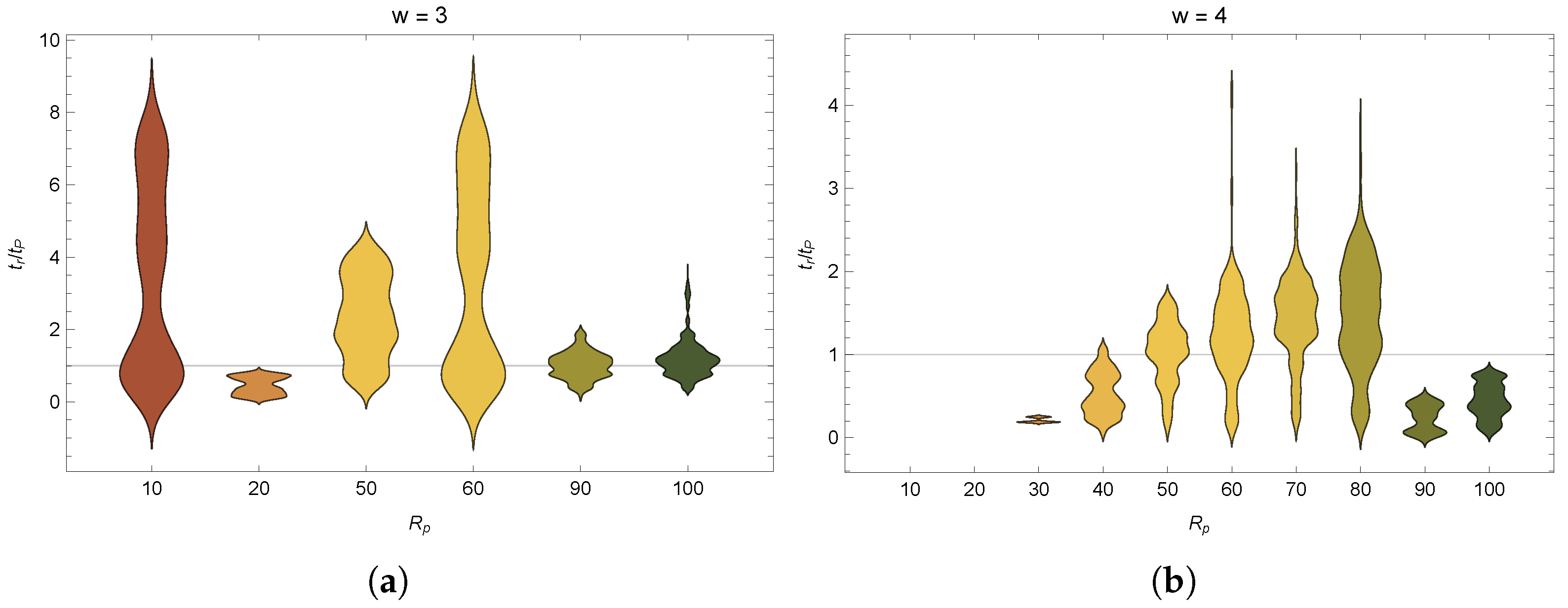
Figure 6 shows the distributions of measured recurrence times for trajectories sampled from state-dependent CA evolved with sets of rules from each classes described in Section 5.1, for widths for and with . All trajectories included in Figure 6 are innovative, and cannot be reproduced by a static ECA rule. Trajectories above the line in each panel are open-ended by Definitions 3 and 4. As expected, no systems with exhibit OEE (since all information is erased and the system immediately converges to a homogeneous state). In some cases generates the largest fraction of open-ended cases, such as for and . However, in other cases it is the state-transition diagrams generated from merging rules with intermediate irreversibility which exhibit the greatest capacity for producing open-ended trajectories.
6.2. Topology of the State-Transition Diagram
To better understand the patterns observed in the dynamics of state-dependent systems across different classes shown in Figure 6, we analyzed the topology of the underlying state-transition diagram for each . Analyses are shown in Table 1, including: , the number of rules in the class (shown in Figure 3); the number of edges in the state-transition graph; , the number of connected components; the size of the largest connected component (LCC); , the mean in-degree of states (same as , the mean out-degree); , the average shortest path length between ordered pairs of states in the LCC; whether or not OEE cases were found (Y or N, respectively), and whether or not the largest connected component is locally physically universal (Y or N, respectively). Cases of interest are highlighted in red and blue, where blue denotes cases that exhibit local physical universality for the largest connected component and red denotes cases that exhibit OEE but are not locally physically universal.
If there is one component and it is locally physically universal the CA is physically universal, and any transformation is possible by suitably preparing the resource and the controller. We do not observe any such cases here for reasons stated above (states containing no information are sinks for the dynamics). However, we do see many cases of local physical universality for large connected components, which dominate the configuration space. For all graphs are locally universal (for all fixed rules r and all w if the graph is locally physically universal, so merging graphs always will yield composite graphs that are also locally universal). In some cases, as with merging individual rule graphs with yields graphs with a single large connected component (excluding only the two homogeneous states), whereas in other cases the merged graph remains fragmented with many disconnected regions, e.g., for . OEE occurs for the former case but not the later, indicating that the larger the locally universal region in configuration space, the higher the propensity for exhibiting OEE. Here, whether a merged graph composed of reversible rules is connected or not is determined by whether the CA is odd or even width, respectively, due to the structure of ECA rules under periodic boundary conditions and is directly related to the number of rules in the set of reversible ones. For other CA, predicting whether the CA will support OEE or not will in general not be so straight forward. For other , the graphs in general have a single connected component that includes all possible states, but these are not locally universal (in all cases this is in part because the all- 0’s and all-1’s states are included in the graph, which are sinks for the dynamics). Nonetheless OEE is still observed in these systems. In general, more edges in the graph (more rules in the state-dependent algorithm)—corresponding to a higher mean degree and lower shortest path—are required to yield OEE for graphs that are not locally universal. That is, if the rules are not reversible, a controller must in general have a greater repertoire of rules to generate OEE than if it uses exclusively reversible rules. For two cases we see local physical universality as an emergent property of the merged graphs (, and , ), but these examples do not exhibit OEE. In both cases the graphs contain a large connected component, meaning that connectivity and the size of the connected region in configuration space together are not sufficient for OEE. None of our topological analyses identify distinctive features of these graphs. Presumably the lack of OEE in these two cases arises due to external constraints: for example resources that terminate in fixed point attractors and thus cannot drive longer recurrence times for .
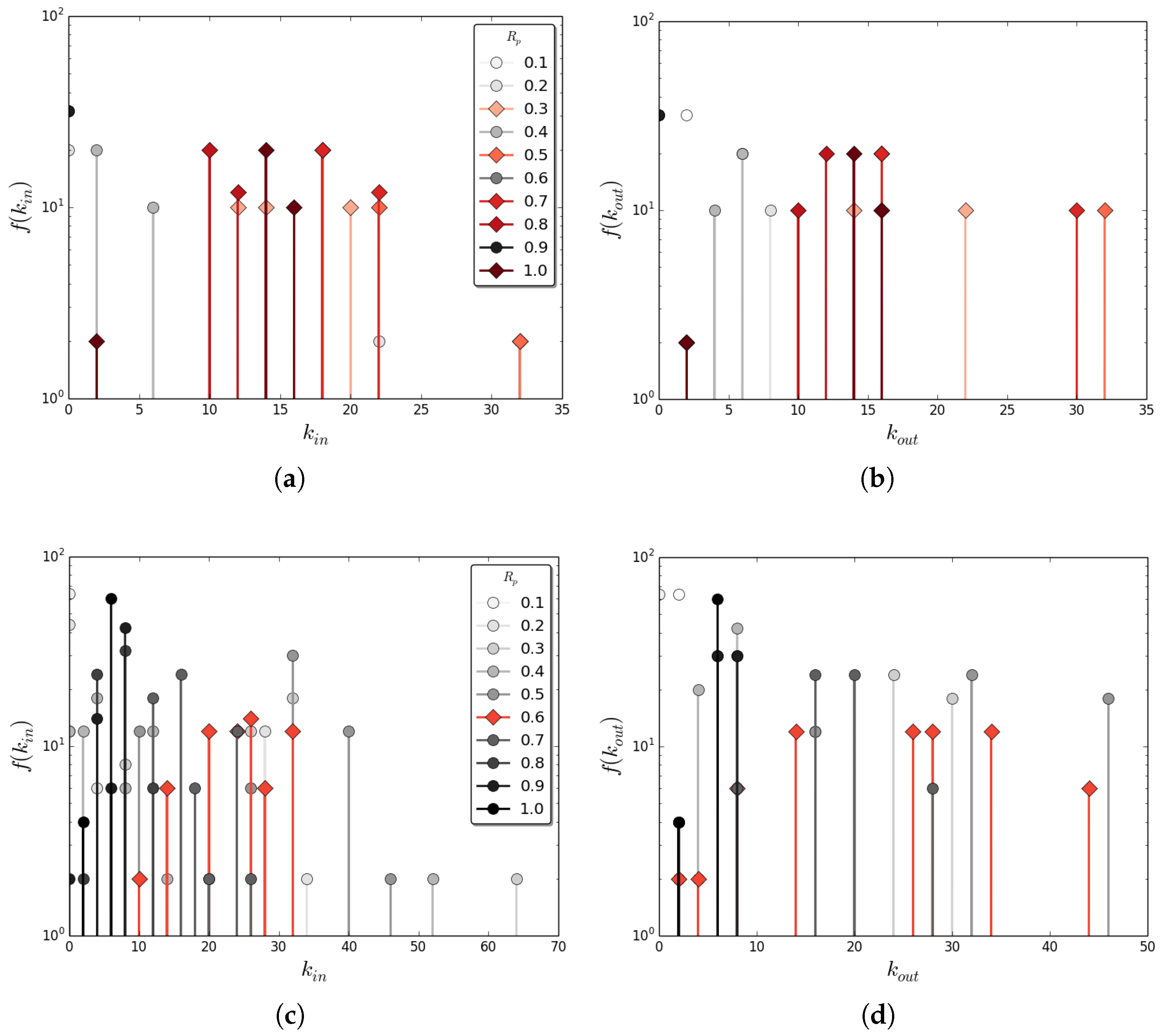
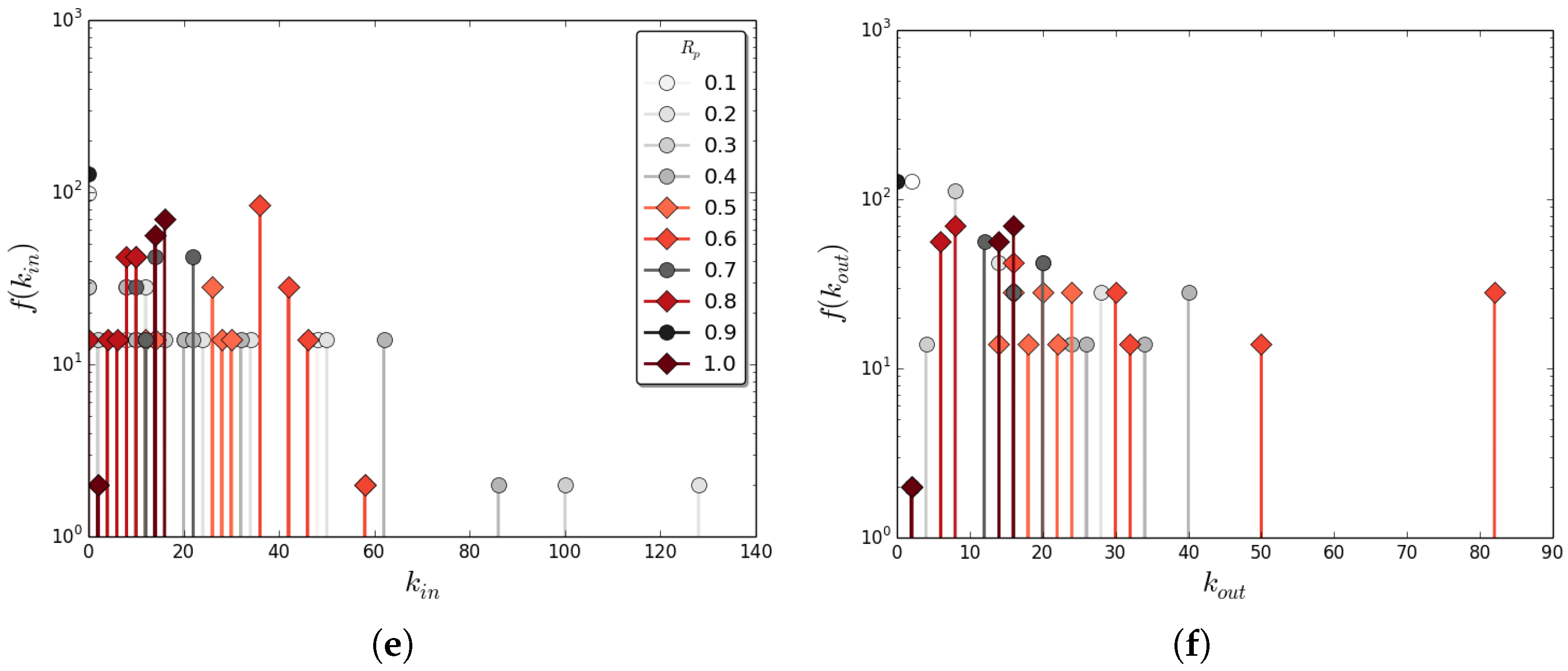
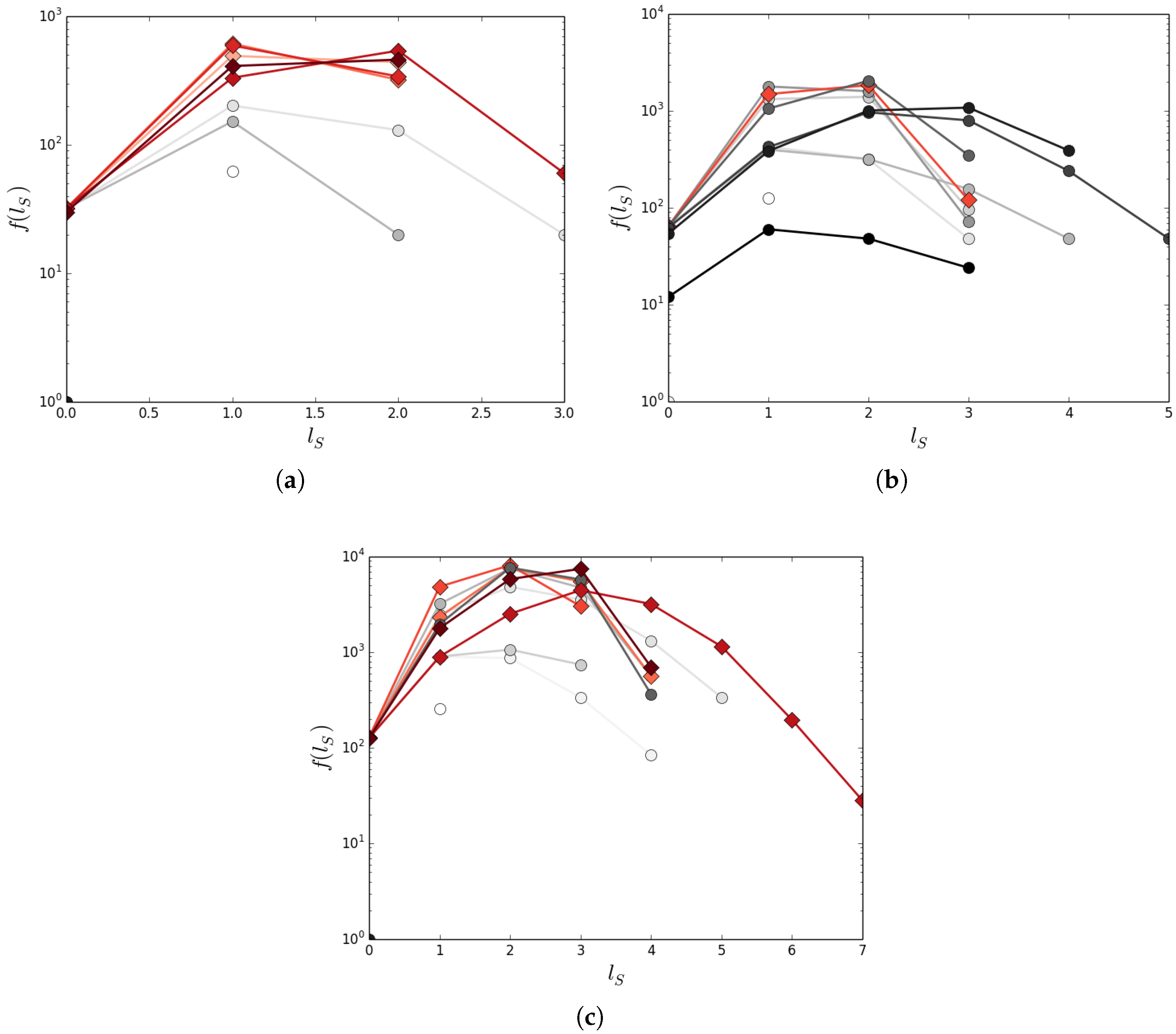
To further explore the relationship between topology, local universality and OEE, we also calculated the distributions of in-degree () and out-degree () for all states, where the in-degree and out-degree quantify how many transformations converge on a state or emanate from it, respectively. We also computed the shortest path between all ordered pairs of states in the largest connected component, to determine the number of transformations necessary to move between any two states (for those with a path between them). Results are shown for state-transition diagrams for , and systems in Figure 7 and Figure 8. In general, we observe that topologies supporting open-ended evolution exhibit a long tail in the out-degree distribution, whereas those where no open-ended cases are observed exhibit a long tail in the in-degree distribution. It is difficult to be conclusive given the small networks implemented in our study, but the general trends suggest that nodes with a high in-degree act as dynamic “sinks” and those with high out-degree as “sources”. In these networks high is associated with high betweenness centrality (see e.g., Figure 4 and Figure 5, statistics not shown), which measures how many shortest paths pass through a given state. The correlation of betweeness centrality with out-degree supports the hypothesis that high-out degree states are sources for the dynamics, enabling more “short-cuts” for transformations between states. State-transition diagrams with many sources can be described as information-generating: due to their interaction with the resource more future paths are possible. By contrast sinks loose information. Physical universality requires a dynamical system where it is possible to move from any state to any other state. Our results show that a few nodes with high out-degree provide short-cuts in the dynamics and therefore may play an important role in enabling physical universality and open-ended evolution. Future work will determine if such networks display small world properties, as is characteristic of many real-world systems [40].
7. Conclusions
It is unknown whether physical universality is a property of our universe. Here we demonstrated a weaker form of physical universality, which we call local physical universality, to provide a framework for understanding cases where true physical universality is not possible or only approximately holds. This may be the case, for example, if the state space cannot be predefined, as proposed by Kauffman [41]. In a system that is locally physically universal, there exists a subset of configurations among which all transformations in the set are possible. Cellular life is often described as an example of a universal constructor (see e.g., [42,43]). This kind of universality is most appropriately cast as a local one. The “universal constructor” (often approximated as the ribosome (see [33] for discussion) operates on a finite set of materials—including amino and nucleic acids among others. An example of a set of configurations which is approximately locally physically universal because of the information-processing architecture of life is the set of proteins composed of the 20 (or so) genetically encoded amino acids: in principle, given sufficient resources a biological system should be able to construct any such protein (or to convert resources from one to another). This example highlights how, when it comes to real physical systems, such as life, approximations to the principle of physical universality (or its local version) may be what is physically relevant.
Our model demonstrates that state-dependent CA can exhibit local physical universality and that these systems can meet the minimal requirements of a formal definition of open-ended evolution. Local physical universality emerges as a result of the connectivity of the underlying state space. Our analysis shows for ECA rule networks, this property is associated with heterogeneity in the in-degree and out-degree of states. It is interesting to speculate how this property relates to real living systems, which are known to exhibit highly heterogenous degree distributions across a variety of systems and scales. One pertinent example is biochemical reaction networks, which exhibit heavy tail degree distributions, with a few hubs dominating network structure [44]. A hub in a biochemical network, such as HO, is hub because it can undergo many chemical transformations. It is possible heterogenous networks emerge not only because of their robustness properties as frequently hypothesized, but also due to their ability to access many configurations. This second hypothesis is consistent with evidence of an increased propensity to innovate due to the structure of gene networks and their ability to quickly traverse phenotype space with relatively few mutations (defined in terms of what reactions are possible) [45,46].
Local physical universality is always a property of reversible rules. However the size of the subset of configuration space that has this property may be small or large depending on the particular dynamical laws (the particular CA rule). In our model, connectivity enabling large regions of configuration space to be locally physically universal can be an emergent property of the state-dependent system (as occurs for irreversible rules), which arises because of the multiplicity of the rules it can access (e.g., the transformations it is programmable to perform). In particular, we equate this property with the particular informational structure of living systems. The advantage of defining local physical universality is that it permits studying systems of varying degrees of universality, and in particular to discuss cases where the ability of systems to increase their repertoire of possible transformations might change in time, as through biological evolution. One could speculate that the biosphere as a whole has trended toward increased connectivity among the possible configurations of material that make up the Earth-system [25], corresponding to better and better approximations to local physical universality. This occurs through evolutionary processes that enable an increasing number of transformations to be mediated by life and its artifacts (such as technology): although the raw materials have always existed on Earth to construct satellites, it is only recently that information processing systems have evolved the capacity to transform those materials into machines and to launch them into space. The framework presented here attempts to explain some of these properties starting from the assumption that the effective laws of physics governing life are state-dependent.
Acknowledgments
This publication was made possible through support of a grant from Templeton World Charity Foundation and the support of the Arizona State University NASA Space Grant. The model and all associated code and data is saved and publicly accessible through GitHub (github.com/alyssa-adams/Reversible_Laws).
Author Contributions
S.I.W., A.M.A. and A.B. conceived and designed the experiments; A.B. performed the experiments; A.M.A., A.B. and S.I.W. analyzed the data; S.I.W., A.M.A, P.C.W.D., and A.B. wrote the paper. All authors have read and approved the final manuscript.
Conflicts of Interest
The authors declare no conflict of interest.
References
- Schrödinger, E. What Is Life? Cambridge University Press: Cambridge, MA, USA, 1944. [Google Scholar]
- Von Neumann, J. Theory of Self-Reproducing Automata; University of Illinois Press: Urbana, IL, USA, 1966. [Google Scholar]
- Clark, E.B.; Hickinbotham, S.J.; Stepney, S. Semantic Closure Demonstrated by the Evolution of a Universal Constructor Architecture in an Artificial Chemistry. J. R. Soc. Interface 2017, 14, 130. [Google Scholar] [CrossRef] [PubMed]
- Ruiz-Mirazo, K.; Peretó, J.; Moreno, A. A universal definition of life: Autonomy and open-ended evolution. Orig. Life Evol. Biosph. 2004, 34, 323–346. [Google Scholar] [CrossRef] [PubMed]
- Marletto, C. Constructor Theory of Life. J. R. Soc. Interface 2015, 12, 20141226. [Google Scholar] [CrossRef] [PubMed]
- Deutsch, D. The Beginning of Infinitiy: Explanations that Transform the World; Penguin: London, UK, 2011. [Google Scholar]
- Deutsch, D. Constructor Theory. Synthese 2013, 190, 4331–4359. [Google Scholar] [CrossRef]
- Janzing, D. Is There a Physically Universal Cellular Automaton or Hamiltonian? arXiv 2010, arXiv:1009.1720. [Google Scholar]
- Schaeffer, L. A Physically Universal Celllular Automaton. In Proceedings of the 2015 Conferences on Innovations in Theoretical Computer Science, Rehovot, Israel, 11–13 January2015. [Google Scholar]
- Salo, V.; Törmä, I. A One-Dimensional Physically Universal Cellular Automaton. In Proceedings of the Conference on Computability in Europe, Turku, Finland, 12–16 June 2017. [Google Scholar]
- Schaeffer, L. A Physically Universal Cellular Automaton. In Proceedings of the International Workshop on Cellular Automata and Discrete Complex Systems, Turku, Finland, 8–10 June 2015. [Google Scholar]
- Adams, A.; Zenil, H.; Davies, P.C.W.; Walker, S.I. Formal Definitions of Unbounded Evolution and Innovation Reveal Universal Mechanisms for Open-Ended Evolution in Dynamical Systems. Sci. Rep. 2017, 7, 997. [Google Scholar] [CrossRef] [PubMed]
- Pavlic, T.P.; Adams, A.M.; Walker, S.I. Self-referencing Cellular Automata: A Model of the Evolution of Information Control in Biological Systems. In Proceedings of the Fourteenth International Conference on the Synthesis and Simulation of Living Systems, New York, NY, USA, 30 July–2 August 2014; pp. 522–529. [Google Scholar]
- Israeli, N.; Goldenfeld, N. Coarse-graining of cellular automata, emergence, and the predictability of complex systems. Phys. Rev. E 2006, 73, 026203. [Google Scholar] [CrossRef] [PubMed]
- Hooft, G. The Cellular Automaton Interpretation of Quantum Mechanics. arXiv 2014, arXiv:1405.1548. [Google Scholar]
- Toffoli, T. Cellular automata as an alternative to (rather than an approximation of) differential equations in modeling physics. Phys. D Nonlinear Phenom. 1984, 10, 117–127. [Google Scholar] [CrossRef]
- Langton, C.G. Computation at the edge of chaos: Phase transitions and emergent computation. Phys. D Nonlinear Phenom. 1990, 42, 12–37. [Google Scholar] [CrossRef]
- Crutchfield, J.P. The calculi of emergence: Computation, dynamics and induction. Phys. D Nonlinear Phenom. 1994, 75, 11–54. [Google Scholar] [CrossRef]
- Borriello, E.; Walker, S.I. An Information-Theoretic Classification of Complex Systems. arXiv 2016, arXiv:1609.07554. [Google Scholar]
- Wolfram, S. A New Kind of Science; Wolfram Media: Champaign, IL, USA, 2002. [Google Scholar]
- Margolus, N. Physics-Like Models of Computation. Phys. D Nonlinear Phenom. 1984, 10, 81–95. [Google Scholar] [CrossRef]
- Conway, J. The Game of Life. Sci. Am. 1970, 223, 4. [Google Scholar]
- Cook, M. Universality in Elementary Cellular Automata. Complex Syst. 2004, 15, 1–40. [Google Scholar]
- Nobili, R.; Pesavento, U. John von Neumann’s automata revisited. In Artificial Worlds and Urban Studies; Istituto Universitario di Architettura: Venezia, Italy, 1994. [Google Scholar]
- Walker, S.I. The Descent of Math. In Trick or Truth? Springer International Publishing: Heidelberg, Germany, 2016; pp. 183–192. [Google Scholar]
- Myhill, J. The Converse of Moore’s Garden-of-Eden Theorem. Proc. Am. Math. Soc. 1963, 14, 685–686. [Google Scholar] [CrossRef]
- Hoel, E.P. When the map is better than the territory. Entropy 2017, 19, 188. [Google Scholar] [CrossRef]
- Kataoka, N.; Kunihiko, K. Functional Dynamics: I: Articulation Process. Phys. D Nonlinear Phenom. 2000, 138, 225–250. [Google Scholar] [CrossRef]
- Kataoka, N.; Kunihiko, K. Functional Dynamics: II: Syntactic Structure. Phys. D Nonlinear Phenom. 2001, 149, 174–196. [Google Scholar] [CrossRef]
- Hofsadter, D. Godel, Escher, Bach: An Eternal Golden Braid; Basic Books: New York, NY, USA, 1979. [Google Scholar]
- Davies, P.C.W.; Walker, S.I. The Hidden Simplicity of Biology: A Key Issues Review. Rep. Prog. Phys. 2016, 79, 102601. [Google Scholar] [CrossRef] [PubMed]
- Goldenfeld, N.; Woese, C. Life Is Physics: Evolution as a Collective Phenomenon Far from Equilibrium. Annu. Rev. Condens. Matter Phys. 2011, 2, 375–399. [Google Scholar] [CrossRef]
- Walker, S.I.; Davies, P.C.W. The Algorithmic Origins of Life. J. R. Soc. Interface 2013, 6, 20120869. [Google Scholar] [CrossRef] [PubMed]
- Mandal, D.; Jarzynski, C. Work and information processing in a solvable model of Maxwell’s demon. Proc. Natl. Acad. Sci. USA 2012, 109, 11641–11645. [Google Scholar] [CrossRef] [PubMed]
- Boyd, A.B.; Crutchfield, J.P. Maxwell demon dynamics: Deterministic chaos, the Szilard map, and the intelligence of thermodynamic systems. Phys. Rev. Lett. 2016, 116, 190601. [Google Scholar] [CrossRef] [PubMed]
- Friston, K. Life as We Know It; Royal Society Publishing: London, UK, 2013; Volume 10, p. 20130475. [Google Scholar]
- Banzhaf, W.; Baumgaertner, B.; Beslon, G.; Doursat, R.; Foster, J.A.; McMullin, B.; Veloso de Melo, V.; Miconi, T.; Spector, L.; Stepney, S.; et al. Defining and simulating open-ended novelty: Requirements, guidelines, and challenges. Theory Biosci. 2016, 135, 131–161. [Google Scholar] [CrossRef] [PubMed]
- Turing, A.M. On computable numbers, with an application to the Entscheidungsproblem. Proc. Lond. Math. Soc. 1937, 2, 230–265. [Google Scholar] [CrossRef]
- Nghe, P.; Hordijk, W.; Kauffman, S.A.; Walker, S.I.; Schmidt, F.J.; Kemble, H.; Yeates, J.M.; Lehman, N. Prebiotic network evolution: Six key parameters. Mol. BioSyst. 2015, 11, 3206–3217. [Google Scholar] [CrossRef] [PubMed]
- Watts, D.J.; Strogatz, S.H. Collective dynamics of ‘small-world’ networks. Nature 1998, 393, 440. [Google Scholar] [CrossRef] [PubMed]
- Kauffman, S.A. Investigations; Oxford University Press: Oxford, UK, 2000. [Google Scholar]
- Danchin, A. Bacteria as computers making computers. FEMS Microbiol. Rev. 2009, 33, 3–26. [Google Scholar] [CrossRef] [PubMed]
- Hickinbotham, S.J.; Stepney, S. Bio-Reflective Architectures for Evolutionary Innovation. In Proceedings of the Artificial Life Conference; MIT Press: Cambridge, MA, USA, 2016; pp. 192–199. [Google Scholar]
- Jeong, H.; Tombor, B.; Albert, A.; Oltvai, Z.N.; Barabási, A.L. The large-scale organization of metabolic networks. Nature 2000, 407, 651–654. [Google Scholar] [PubMed]
- Ciliberti, S.; Olivier, C.M.; Wagner, A. Innovation and robustness in complex regulatory gene networks. Proc. Natl. Acad. Sci. USA 2007, 104, 13591–13596. [Google Scholar] [CrossRef] [PubMed]
- Wagner, A. Arrival of the Fittest: Solving Evolution’s Greatest Puzzle; Penguin: New York, NY, USA, 2014. [Google Scholar]
Figure 1.
Examples of state-transition diagrams for Elementary Cellular Automata (ECA) with periodic boundary conditions. Shown are the rule table and state-transition diagram for ECA rules 110 (a,c), respectively, and 240 (b,d), respectively. Garden of eden states are highlighted in red. Rule 240 has no garden of eden states and is logically reversible. Each loop in the state transition diagram of rule 240 represents a set of configurations that is locally physically universal (see text), whereas this property does not hold for rule 110.

Figure 2.
A state-dependent cellular automaton composed of two spatially segregated interacting parts as shown in (b): a system () is coupled to a resource (program) () through a “metarule” that controls the interaction, illustrated abstractly in (a). The metarule is a function that maps the states of the systems S and P to a new update rule for S.
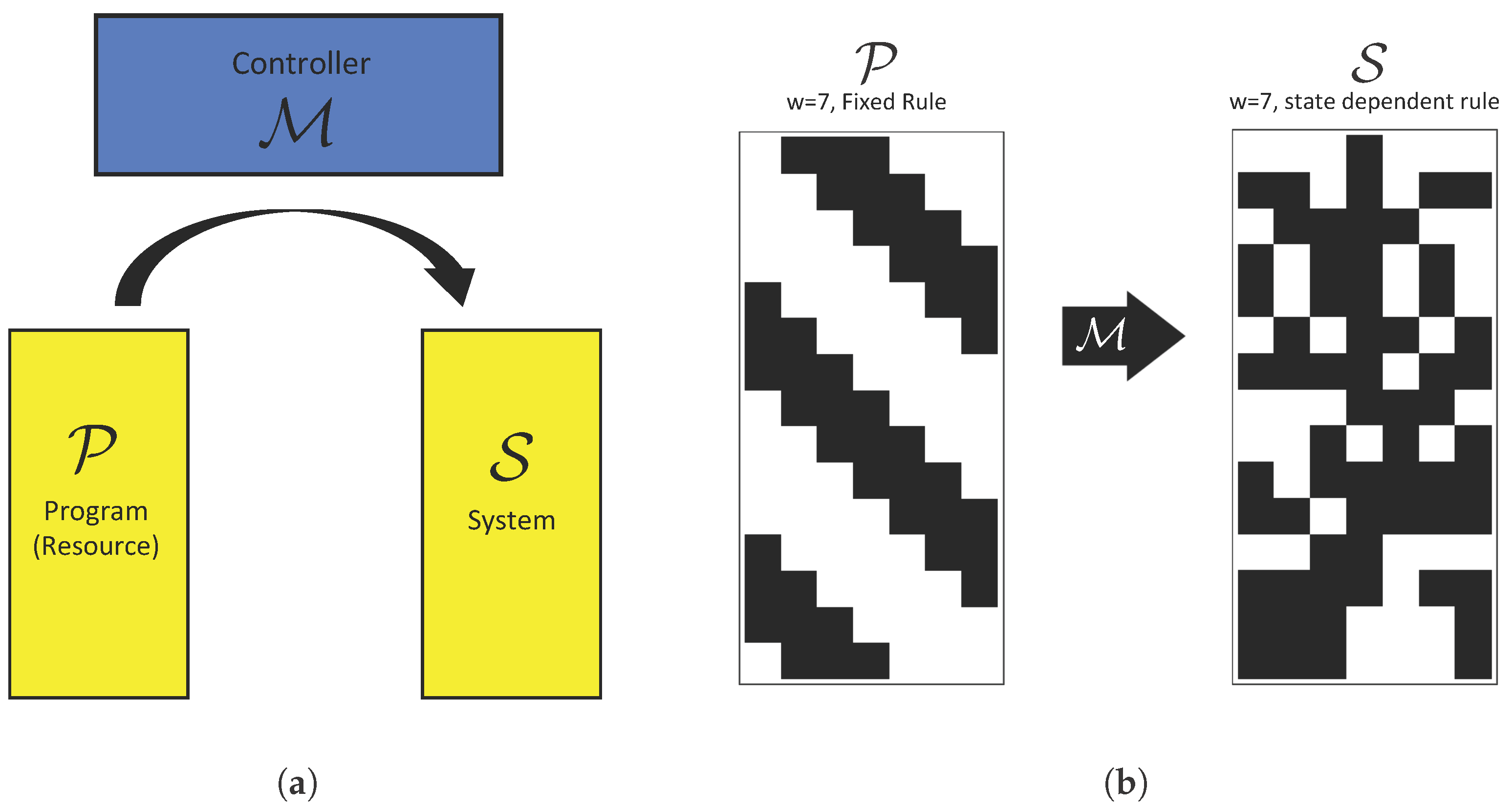
Figure 3.
The relative size of all sets (as percentages here) for ECA widths . Different w are denoted by concentric circles, where colors indicate separate sets.
Figure 3.
The relative size of all sets (as percentages here) for ECA widths . Different w are denoted by concentric circles, where colors indicate separate sets.

Figure 4.
State transition diagrams for for varying w. Node size is weighted by out-degree and colors indicate betweenness centrality (high values are warm, low values cool tones). Each connected component is locally physically universal.
Figure 4.
State transition diagrams for for varying w. Node size is weighted by out-degree and colors indicate betweenness centrality (high values are warm, low values cool tones). Each connected component is locally physically universal.

Figure 5.
State transition diagrams for with with varying . Node size is weighted by out-degree and colors indicate betweenness centrality (high values are warm, low values cool tones).
Figure 5.
State transition diagrams for with with varying . Node size is weighted by out-degree and colors indicate betweenness centrality (high values are warm, low values cool tones).

Figure 6.
Distributions of recurrence times (relative to the Poincaré recurrence time , y-axis) of sampled systems with state trajectories that are innovative, meaning they are not reproducible by any static-rule ECA according to Definition 4. Trivial state-trajectories consisting of all 1’s or 0’s were removed. Distributions are shown for all sets (x-axis) of a given CA widths w (panels a–e). The horizontal line represents where . State-trajectories above this line are classified as open-ended according to Definition 3.

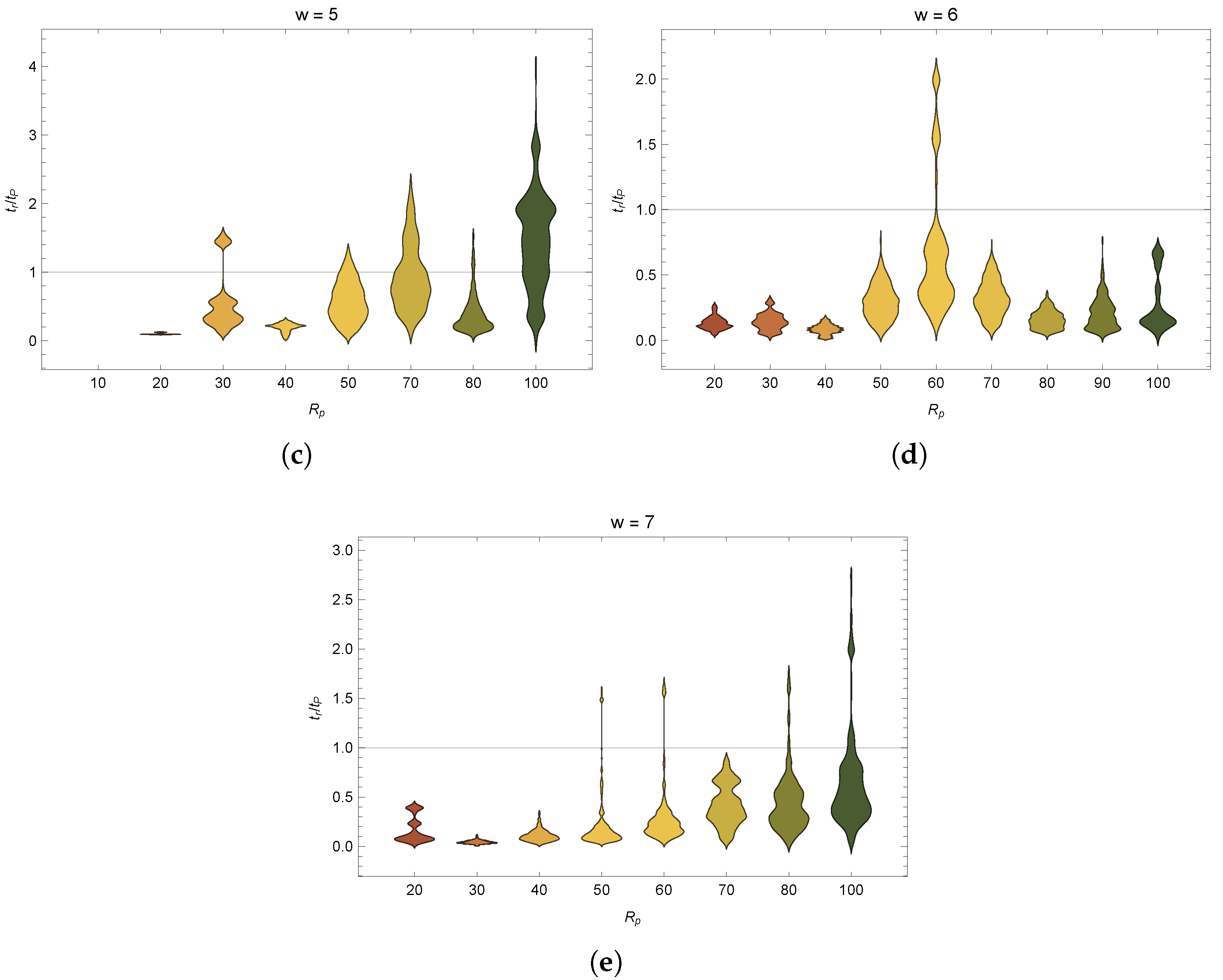
Figure 7.
Frequency distribution of the in-degree (, (a,c,e)) and out-degree (, (b,d,f)) for state-transition diagrams for varying for widths (a,b), (c,d) and (e,f). State-transition diagrams with sampled trajectories exhibiting open-ended dynamics are shown in red, while those where no open-ended cases were confirmed are shown on a gray scale.


Figure 8.
Shortest path () for state-transition diagrams for varying for widths (a), (b) and (c). State-transition diagrams with sampled trajectories exhibiting open-ended dynamics are shown in red, while those where no open-ended cases were confirmed are shown on a grey scale.
Figure 8.
Shortest path () for state-transition diagrams for varying for widths (a), (b) and (c). State-transition diagrams with sampled trajectories exhibiting open-ended dynamics are shown in red, while those where no open-ended cases were confirmed are shown on a grey scale.


Table 1.
Statistics of the topology for state-transition diagrams for of widths . Bold highlighting indicates state-transition graphs that permit OEE or are that have a largest connected component that is locally universal. Included are: , the number of rules in the class ; the number of edges in the state-transition graph; , the number of connected components of the graph; the size of the largest connected component (LCC); , the mean in-degree of states (same as ); , the average shortest path length between directed pairs of states in the LCC; whether or not OEE cases were found (Y or N, respectively), and whether or not the largest connected component is locally physically universal (Y or N, respectively).
| , w | OEE | |||||||
|---|---|---|---|---|---|---|---|---|
| , | 2 | 64 | 1 | 100% | 13 | 0.65 | N | N |
| , | 8 | 204 | 1 | 100% | 41 | 1.35 | N | N |
| , | 30 | 524 | 1 | 100% | 105 | 1.42 | Y | N |
| , | 8 | 164 | 1 | 100% | 33 | 0.94 | N | N |
| , | 66 | 644 | 1 | 100% | 129 | 1.3 | Y | N |
| , | 106 | 624 | 1 | 100% | 125 | 1.32 | Y | N |
| , | 20 | 344 | 1 | 100% | 69 | 1.65 | Y | N |
| , | 16 | 444 | 2 | 94% | 89 | 1.48 | Y | Y |
| , | 2 | 128 | 1 | 100% | 21 | 0.66 | N | N |
| , | 8 | 428 | 1 | 100% | 71 | 1.41 | N | N |
| , | 36 | 1368 | 1 | 100% | 228 | 1.52 | N | N |
| , | 8 | 420 | 1 | 100% | 70 | 1.72 | N | N |
| , | 72 | 1848 | 1 | 100% | 308 | 1.48 | N | N |
| , | 72 | 1548 | 1 | 100% | 258 | 1.57 | Y | N |
| , | 36 | 1088 | 1 | 100% | 181 | 1.76 | N | N |
| , | 8 | 428 | 2 | 97% | 71 | 2.34 | N | N |
| , | 8 | 428 | 3 | 84% | 71 | 2.46 | N | Y |
| , | 6 | 368 | 8 | 18% | 61 | 1.58 | N | Y |
| , | 2 | 256 | 1 | 100% | 36 | 0.66 | N | N |
| , | 8 | 900 | 1 | 100% | 129 | 1.72 | N | N |
| , | 28 | 2524 | 1 | 100% | 361 | 2.35 | N | N |
| , | 8 | 956 | 1 | 100% | 137 | 1.85 | N | N |
| , | 40 | 3280 | 1 | 100% | 469 | 2.14 | N | N |
| , | 26 | 2440 | 1 | 100% | 349 | 2.25 | Y | N |
| , | 100 | 4960 | 1 | 100% | 709 | 1.87 | Y | N |
| , | 20 | 1964 | 2 | 98% | 281 | 2.26 | N | Y |
| , | 8 | 900 | 2 | 98% | 129 | 3.11 | Y | N |
| , | 16 | 1908 | 2 | 98% | 273 | 2.43 | Y | Y |
© 2017 by the authors. Licensee MDPI, Basel, Switzerland. This article is an open access article distributed under the terms and conditions of the Creative Commons Attribution (CC BY) license (http://creativecommons.org/licenses/by/4.0/).
Share and Cite
MDPI and ACS Style
Adams, A.M.; Berner, A.; Davies, P.C.W.; Walker, S.I. Physical Universality, State-Dependent Dynamical Laws and Open-Ended Novelty. Entropy 2017, 19, 461. https://doi.org/10.3390/e19090461
AMA Style
Adams AM, Berner A, Davies PCW, Walker SI. Physical Universality, State-Dependent Dynamical Laws and Open-Ended Novelty. Entropy. 2017; 19(9):461. https://doi.org/10.3390/e19090461
Chicago/Turabian StyleAdams, Alyssa M., Angelica Berner, Paul C. W. Davies, and Sara I. Walker. 2017. "Physical Universality, State-Dependent Dynamical Laws and Open-Ended Novelty" Entropy 19, no. 9: 461. https://doi.org/10.3390/e19090461
Note that from the first issue of 2016, this journal uses article numbers instead of page numbers. See further details here.