Second-Law Analysis of Irreversible Losses in Gas Turbines


1
Center of Applied Space Technology and Microgravity (ZARM), the University of Bremen, 28359 Bremen, Germany
2
Institute of Engineering Thermophysics, Chinese Academy of Sciences, Beijing 100190, China
3
University of Chinese Academy of Sciences, Beijing 100049, China
*
Authors to whom correspondence should be addressed.
Entropy 2017, 19(9), 470; https://doi.org/10.3390/e19090470
Submission received: 26 July 2017
/
Revised: 29 August 2017
/
Accepted: 31 August 2017
/
Published: 4 September 2017
(This article belongs to the Special Issue Entropy in Computational Fluid Dynamics)
Abstract
:Several fundamental concepts with respect to the second-law analysis (SLA) of the turbulent flows in gas turbines are discussed in this study. Entropy and exergy equations for compressible/incompressible flows in a rotating/non-rotating frame have been derived. The exergy transformation efficiency of a gas turbine as well as the exergy transformation number for a single process step have been proposed. The exergy transformation number will indicate the overall performance of a single process in a gas turbine, including the local irreversible losses in it and its contribution to the exergy obtained the combustion chamber. A more general formula for calculating local entropy generation rate densities is suggested. A test case of a compressor cascade has been employed to demonstrate the application of the developed concepts.
1. Introduction
A gas turbine is a type of combustion engine, which usually comprises an upstream compressor, a downstream turbine, and a combustion chamber in between. The design of a high performance gas turbine is a key technology in modern industry due to its significant applications in aircraft, electrical generators, and ships.
Compared to reciprocating engines, gas turbines have the advantages of a higher power-weight ratio, a smaller volume, lower toxic emissions, etc. However, the efficiency of gas turbines is usually lower than that of reciprocating engines. Generally, the efficiency of a gas turbine can be improved by increasing the pressure ratio [1] and reducing the engine weight [2]. However, according to the second law of thermodynamics, the efficiency of a gas turbine is ultimately determined by the irreversibility in its flow and temperature field. For example, if a gas turbine has a pressure ratio of 20, its efficiency according to an ideal Brayton cycle is about 60%, whereas the efficiency even for a modern gas turbine is no more than 40%. A gas turbine may be combined with a steam plant to form a “combined cycle” system. In recent years, the efficiency of the gas turbine combined cycle system’s power generation has been increased to 60% [3]. However, this only increases the system’s overall efficiency, while the efficiency of the gas turbine is not really improved. The key to improving the efficiency of a gas turbine still lies in how to reduce the losses due to irreversibility.
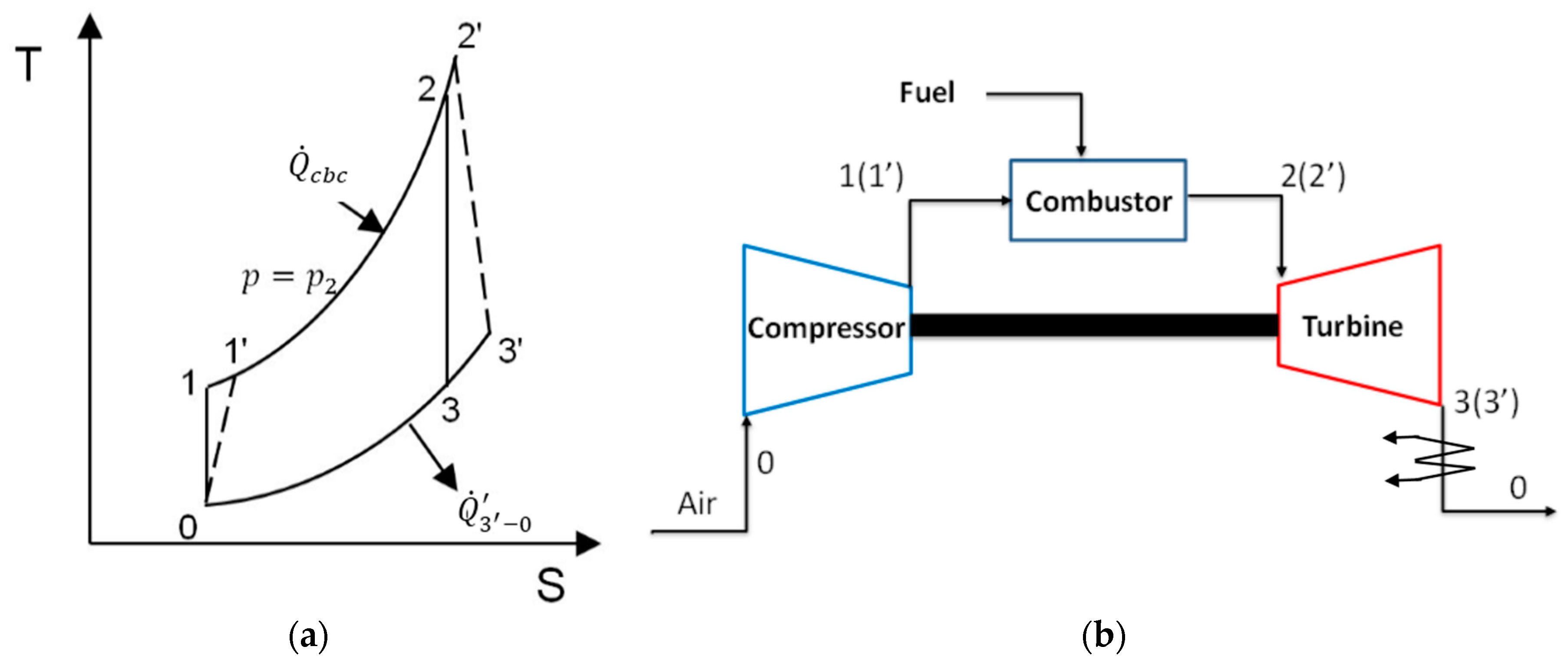
In an ideal gas turbine, the working gases follow the Brayton cycle, which is composed of the procedures of isentropic compression, isobaric (constant pressure) combustion, isentropic expansion, and isobaric heat rejection: see the cycle 0–1–2–3–0 in Figure 1. The efficiency for the ideal Brayton cycle is:
where and are the heat generation and release rates in the processes of isobaric combustion (1–2) and isobaric heat rejection (3–0).
However, irreversibility occurs in a real gas turbine. The T-S diagram for a real Brayton cycle is indicated by 0–1’–2’–3’–0 in Figure 1, in which only the irreversibility of the compression (0–1’) and expansion (2’–3’) processes are taken into account. The efficiency of the real Brayton cycle is
When the compressor and the turbine are considered to be adiabatic, the entropy will increase in processes 0–1’ and 2’–3’ due to irreversibility, leading to higher entropy at state 3’ than at state 3. As a result, the heat release in process 3’–0 is larger than in the ideal cycle (3–0), i.e., . Thus, the efficiency of a real gas turbine is always lower than that of an ideal one.
The second-law analysis (SLA) is a very helpful tool for understanding these irreversible processes. In the SLA, irreversibility in both flow and temperature fields are accounted for. However, the SLA was usually used for analyzing a thermal system, while the detailed flow and temperature fields were traditionally studied within the disciplines of fluid mechanics and heat transfer, in which the SLA still has not received much attention. Entropy almost never appears in the text books of fluid dynamics and heat transfer: see [4,5] as examples. This concept is ignored perhaps due to the reason that the irreversibility effect is considered to be not important in these two disciplines. However, turbulent flow and heat transfer are typical irreversible processes due to the dissipation in the flow field and irreversibility in the temperature fields. Another possible reason is that it is very difficult to calculate or measure the local entropy generation rate accurately due to model and experimental errors.
Some progress has been made in employing the SLA in flow and heat transfer problems since the 1980s. Bejan [6,7] laid the foundation with respect to analyzing and optimizing thermal systems with the SLA approach. Kock and Herwig [8] extended this concept to a detailed analysis of turbulent flows, and identified four different mechanisms of entropy generation: dissipation in a mean and fluctuating velocity field and heat flux in a mean and fluctuating temperature field. Later, Kock and Herwig [9] developed equations for computing entropy generation rates for Reynolds Averaged Navier–Stokes Simulations (RANSs) and implemented them into computational fluid dynamics (CFD) codes. Jin and Herwig [10] indicated that model errors in RANS simulations may lead to considerable uncertainties in entropy generation results.
With the development of high performance computers in recent years, people have started to calculate the losses in blade cascades from RANS results. Orhan [11] investigated the loss mechanism of an axial turbine cascade with the SLA. Denton and Pullan [12] and Zlatinov et al. [13] analyzed the local entropy generation rate in turbines with unsteady RANSs. However, Kopriva et al. [14,15] found that RANSs have much lower accuracy than large eddy simulations (LESs). Tucker [16,17] indicated that it is particularly difficult to predict unsteady separations in turbines with RANSs. As a compromise between the computational cost and the accuracy, Lin et al. [18] studied the local entropy generation in a turbine cascade passage with a delayed detached eddy simulation (DDES) method. The losses in both flow and temperature fields were visualized according to the numerical results. With the same method, Wang et al. [19] analyzed the interaction between the corner separation and wakes in a compressor cascade. The detailed coherent structures, local losses information, and turbulence characteristics were identified according to the local entropy generation rate. Despite this progress, more systematic studies are still required for understanding the irreversible processes in gas turbines. In particular, the relationship between local entropy generation and global efficiency should be better understood.
In the present paper, we attempt to investigate several fundamental concepts with respect to the SLA of the irreversible processes in gas turbines. Entropy and exergy transport equations for compressible flows in a rotating frame will be derived in Section 2. Through the derivation, we will show the relationship between the SLA and the other laws in fluid mechanics. In Section 3, we will discuss the dimensionless coefficients for assessing irreversible processes in a gas turbine. The concepts of exergy transformation efficiency and exergy transformation number will be introduced. CFD modeling for calculating the local entropy generate rate density will be discussed in Section 4. A test case for applying the developed theories will be provided in Section 5. The conclusions are given in Section 6.
2. The Entropy and Exergy Transport Equations for Compressible Flows in a Rotating Frame
The governing equations for the flows in a cascade passage or the combustion chamber are the compressible Navier–Stokes and energy equations. The equations in a rotating frame were adopted, and thus they can be also used for the flows in rotors. The governing equations [20,21] read:
The chemical reaction in the combustion chamber is not considered here for simplicity, while the combustion heat is accounted for by the heat exchange at the boundary walls. The reference frame rotates with the angular velocity of . The value of is zero when a stationary frame is under consideration. The reference frame velocity is , where is the displacement from the axis to the position vector . If is selected as the axis, we have . is the component of the body acceleration rate vector , in which the Coriolis and centrifugal forces are taken into account.
, , , and are the density, frame velocity component, relative velocity component, temperature, and thermal conductivity, respectively. The relative total energy and enthalpy are calculated by and , respectively. is the anisotropic part of the viscous stress tensor, where the strain rate .
Multiplying Equation (4) with and considering , the transport equation of the relative kinetic energy can be derived:
where . Subtracting Equation (6) from Equation (5), the transport equation of the enthalpy can be obtained, i.e.,
Substituting Equation (7) into the fundamental equation of thermodynamics , the entropy equation can be derived, i.e.,
The irreversibility is due to the last two terms in Equation (8), which are always positive. They are called the entropy generation rate density in the temperature field and in the flow field . Their definitions are:
For an open system, the total differential of exergy of a gas is , where is the environmental temperature, is the specific exergy of a gas, and is the total kinetic energy. The transport equation of can be obtained from Equation (4), i.e.,
Substituting Equations (7), (8), and (10) into the total derivative of exergy, the balance equation of exergy can be obtained, i.e.,
Equations (8) and (11) were derived for compressible flows in a rotating frame, but they can also be used for incompressible flows in a non-rotating frame when is a constant and is zero.
Integrating Equations (8) and (11) in a volume under consideration, e.g., a cascade passage or the combustion chamber, the integral forms of the entropy and exergy equations can be obtained. They are:
where is the overall entropy generation rate in domain , is the direction vector of a surface element, is the exchange of entropy due to heat transfer at the boundary, is the shaft work when a rotor is accounted for, and is the increase of exergy due to heat transfer. When the compressor and turbine are assumed to be adiabatic, is non-zero only in the combustion chamber.
Equation (12) shows that the entropy will always increase or remain constant in an isolated system in which and are zero. The corresponding destruction of exergy according to Equation (13) is . This is accordance with the second law of thermodynamics. The derivation shows that the traditional laws in fluid mechanics and heat transfer are sufficient for satisfying the second law of thermodynamics. It is not necessary to solve the entropy or exergy equations in numerical simulations. The entropy generation rate can be calculated as post processing of the numerical results.
3. Dimensionless Coefficients for Assessing Irreversible Processes
The bulk quantitates , , , and can be calculated by the statistics of the local flow quantities , , , and , respectively. For example, the bulk temperature is calculated by , where is the cross section under consideration. The mass flow rate is . The losses in a certain process step, such as in a cascade passage, can be evaluated with these bulk quantities.
The loss in a cascade passage was traditionally evaluated by the enthalpy loss coefficient [22], which is defined by:
where is the rate of specific enthalpy, and the subscripts “” and “” denote the outlet and isentropic process, respectively. The superscript * denotes the stagnation value.
In a real application, instead of Equation (14), it is more convenient to use the stagnation pressure loss coefficient [22] instead of to indicate the loss, i.e.,
where the subscript “” denotes the inlet. Obviously, the irreversibility due to heat transfer is not taken into account in Equations (14) and (15). However, as shown in Figure 1, the increase of entropy due to heat transfer will also reduce the efficiency of a gas turbine. The losses in a cascade can be more accurately assessed by the SLA. Denton [23] suggested the use of an entropy loss coefficient to indicate the loss of efficiency in a cascade, i.e.,
where is the entropy generation rate in a cascade under consideration. The losses of exergy due to irreversibility are more accurately assessed by Equation (16) than by Equation (15). However, the contribution of the cascade to the output work is not taken into account by Equation (16). According to Equation (16), the optimized blade cascades should have low loading and work at a small incidence angle, thus the entropy generation can be minimized. This conflicts with some real applications in which higher loading blade cascades which work at higher incidence angles are preferred.
In order to assess the irreversible processes in gas turbines more comprehensively, we adopted and further developed the concepts of entropic potential and energy devaluation number, which have been proposed by Herwig and his colleagues [24,25,26] in recent years. According to these studies, the entropic potential is defined by the entropy generation rate by which the entropy of the ambient is increased when the primary energy rate becomes part of its internal energy, i.e.,
where is the environmental temperature. The amount of the entropic potential rate of that is consumed by the process step i under consideration can be determined by the energy devaluation number, which is defined by
More details can be found in [24,25,26].
In a gas turbine, the primary energy is the exergy which is obtained in the combustion chamber in process 1’–2’. was derived and defined in Equation (13). In order to simplify its calculation, we approximate the local wall temperature in the combustion chamber with the bulk temperature in the cross section which is enclosed by the wall surface. Thus, the primary energy can be calculated by
where is the exergy obtained in the combustion chamber, and is the mass flow rate.
Time averaging and summing up the integral exergy equations (Equation (13)) of all the processes in a gas turbine and dividing it with , we have
as the chain of energy devaluation and transportation. In this chain, is the energy devaluation number of process i defined by Equation (18). The exergy obtained in the combustion chamber is devaluated by , transformed to shaft work by , or transported to the environment by . occurs in process (see Figure 1) due to the release of heat, which is not a real loss of exergy and this part of exergy can be (totally by an ideal process and partly by a real process) regained through a gas turbine combined cycle (GTCC) power generation system. Thus, the exergy transformed by the gas turbine is . Multiplying Equation (20) with , we may define the exergy transformation efficiency of a gas turbine by:
indicates the fraction of the heat which can be transformed to exergy. is higher than defined by Equation (2) by .
is influenced by both the entropy generation rate in each process step i and its contribution to . Thus, we may define the exergy transformation number of process step i by:
where is the contribution of process i to . That is to say, although all of the exergy is obtained in the combustion chamber, the combustion chamber is not the only contributor to . The compressor upstream also has important effects on .
When of each process is known, we have as the chain of exergy transformation. In a gas turbine, we use , , and to denote the exergy transformation numbers of turbine cascade i, compressor cascade i, and the combustion chamber.
of turbine cascade i is determined only by the entropy generation rate in it, i.e.,
Compressor cascade i may have two opposite effects on exergy transformation. On the one hand, similar to a turbine cascade, the exergy is destroyed due to entropy generation. On the other hand, the exergy obtained in the combustion chamber is increased due to the increase of the temperature and the pressure through the compressor cascade. Under this consideration, is calculated by
where is the entropy generation rate in compressor cascade i, and is the contribution of compressor cascade i to the exergy obtained in the combustion chamber . Figure 2 shows the influence of compressor cascade i on the exergy obtained in the combustion chamber schematically: the static temperature is increased from to through compressor cascade i. The potential exergy that can be obtained in the combustion chamber through a reversible process is increased from to . and are the temperature at the exit of the combustion chamber when the temperature at the inlet of the combustion chamber is and , respectively. Thus, the contribution of compressor cascade i to is calculated by
with and being determined according to the first law of thermodynamics, by
When an ideal gas with a constant capacity is taken into account, Equations (25) and (26) can be simplified to
of the combustion chamber is calculated by
where is the entropy generation rate in the combustion chamber, and is the increase of exergy in the combustion chamber without the upstream compressor through a reversible process. It is calculated by
where is the compressor inlet temperature (state 0 is indicated in Figure 1), and is temperature at the exit of the combustion chamber when the inlet temperature of the combustion chamber is . Obviously, we have .
When the efficiency coefficients of all the processes are known, we have
as a chain of exergy transformation. The exergy transformation number can be used to assess an isolated process step, since only local flow and temperature fields are needed to calculate its value.
4. Modeling of Local Entropy Generation Rate Densities
The entropy generation rate densities and can be directly calculated from direct numerical simulation (DNS) results. However, DNS requires very high computational costs and is thus not suitable for engineering applications. When RANS or other models’ results are used in the study, part of the losses cannot be calculated directly and thus must be modeled. Kock and Herwig [8,9] proposed models for calculating entropy generation rates with RANS results. In these models, and were decomposed by:
where is the turbulent dissipation rate, and is the temperature fluctuation dissipation rate. However, and are not always calculated explicitly in RANS models, and even when they are determined, their accuracies are low since they often are only used as intermediate quantities for calculating the eddy viscosity or Reynolds stresses: see [27].
Instead, we assume that, when the flow domain under consideration is sufficiently large, the produced turbulence is in balance with the dissipation, i.e.,
With this assumption, and can be replaced with the turbulence production rate and the temperature fluctuation production rate . According to the eddy viscosity hypothesis, the effect of turbulence on momentum and heat transfer can be approximated in a similar way as the molecular diffusion: see [27]. Thus, and can be calculated by
where is the eddy viscosity, and is the turbulent thermal conductivity. is the turbulent Prandtl number. Equations (35) and (36) can be calculated directly in all RANS models which are based on the eddy viscosity hypothesis.
5. A Test Case of Application
As an example for applying the concepts developed in Section 2, Section 3 and Section 4, we analyzed the turbulent flow in an isolated compressor cascade which was taken from the experimental database of [28] with a RANS method. Through this low cost test case, we will show how to analyze the numerical results with the concepts developed in Section 2, Section 3 and Section 4.
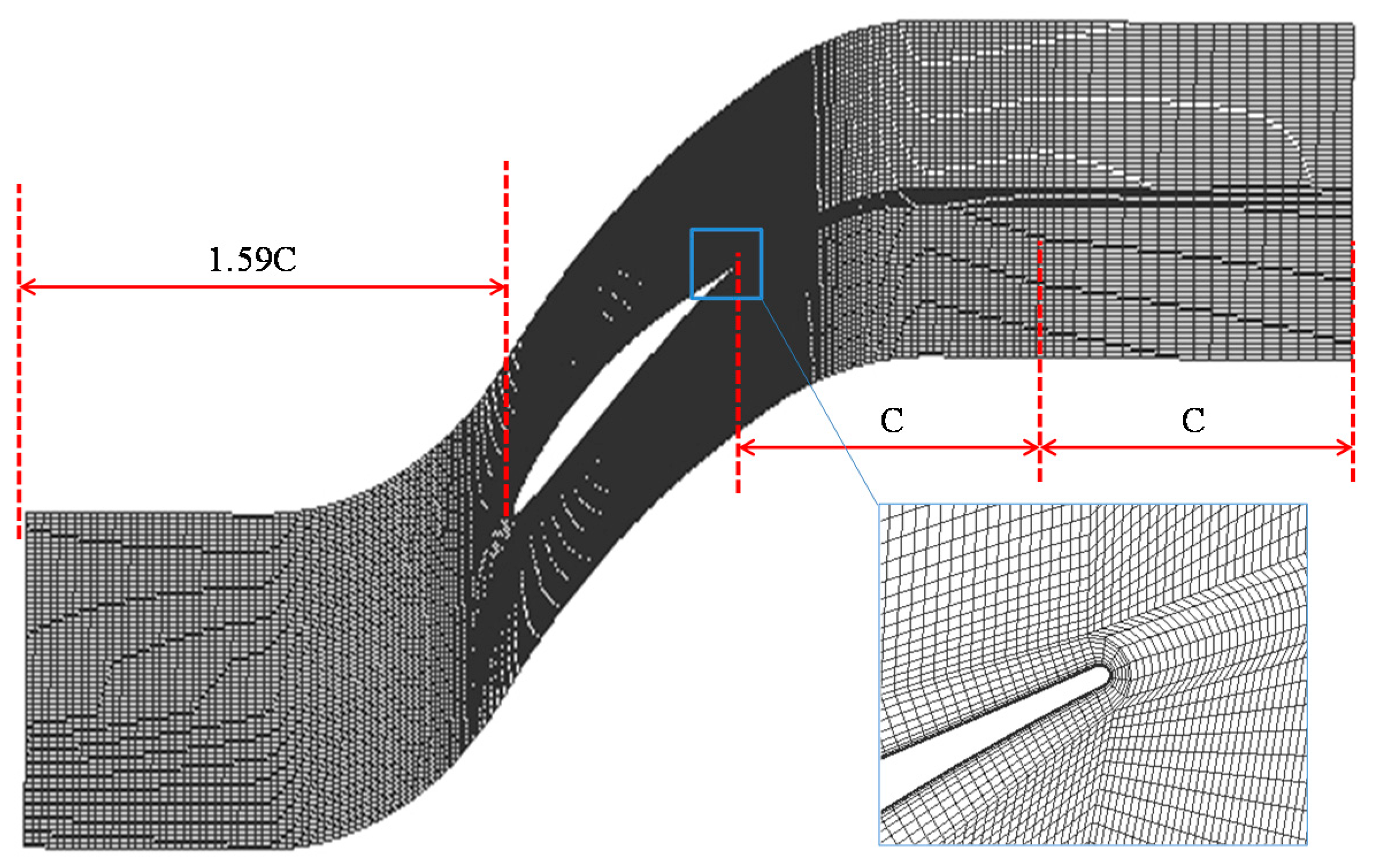
The computational domain is half of the cascade passage. The geometric parameters of the cascade are shown in Table 1. In order to reduce the boundary effects, the inlet and outlet regions were extended by 1.59C and 2C, respectively, where C is the length of the chord. The velocity profile at the inlet was given according to the experimental data in [28]. The time and surface averaged inlet velocity and turbulent intensity are 40 ms−1 and 0.8%, respectively. The turbulent intensity was calculated by , where is the inlet turbulent kinetic energy. The inlet-specific dissipation rate is s−1. Four incidence angles were accounted for in the present study. They are 0°, 2°, 4°, and 7°. Since the flow is at a small velocity (the Mach number is smaller than 0.3), the fluid in the cascade is assumed to be incompressible with the constant density of 1.217 kg m−3.
The flow was assumed to be quasi-steady. The following steady Reynolds averaged Navier–Stokes equations were solved during the simulation:
The eddy viscosity was calculated with the k-ω Shear-Stress Transport (SST) turbulence model [29].
An open source CFD software, OpenFoam v16.06+, was used to carry out the simulation. PimpleFoam was selected as the computational solver. This solver is based on a pressure correction method for incompressible flows. The second-order upwind scheme was used for spatial discretization. Body-fitted mesh, which concentrates near the wall, was adopted in the study. The dimensionless mesh spacing of the first grid point near the wall is ensured to be smaller than 1 to resolve the turbulent boundary layer. The mesh in the region close to the cascade’s trailing edge was refined to capture the corner separation. The mesh in a cross section is shown in Figure 3. A typical mesh has about 5.8 million grid points. The mesh independence study was performed to ensure the results are mesh resolution independent. More computational details can be found in [30].
The entropy generation in the temperature field was neglected in the present test case, since it is much smaller than the one in the flow field. The global static temperature at the inlet and outlet were approximated according to the ideal gas law, i.e., . The specific gas constant is 287.1 J kg−1 K−1. Since the density is a constant, the global temperature is proportional to the global static pressure.
The entropy generation rate density in the flow field was calculated with Equations (31) and (35). When Equation (31) is adopted, the turbulent dissipation rate must be determined corresponding to the specific turbulent model. For the k-ω SST turbulence model in use, is calculated by
where is the constant used in the k-ω SST turbulence model. It is determined empirically according to experimental and DNS data. Reference [28] suggests its value to be 0.09.
The static pressure coefficient at two sections ( and 29.7%) are shown in Figure 4. The gap between the current CFD results and the experimental data in [28] is due to the model error. The accuracy can be further improved by using more accurate CFD methods, e.g., the large eddy simulation (LES) method. However, the current low cost CFD method is sufficient for the purpose of this study, i.e., demonstrating how to analyze cascade flows with the developed concepts.
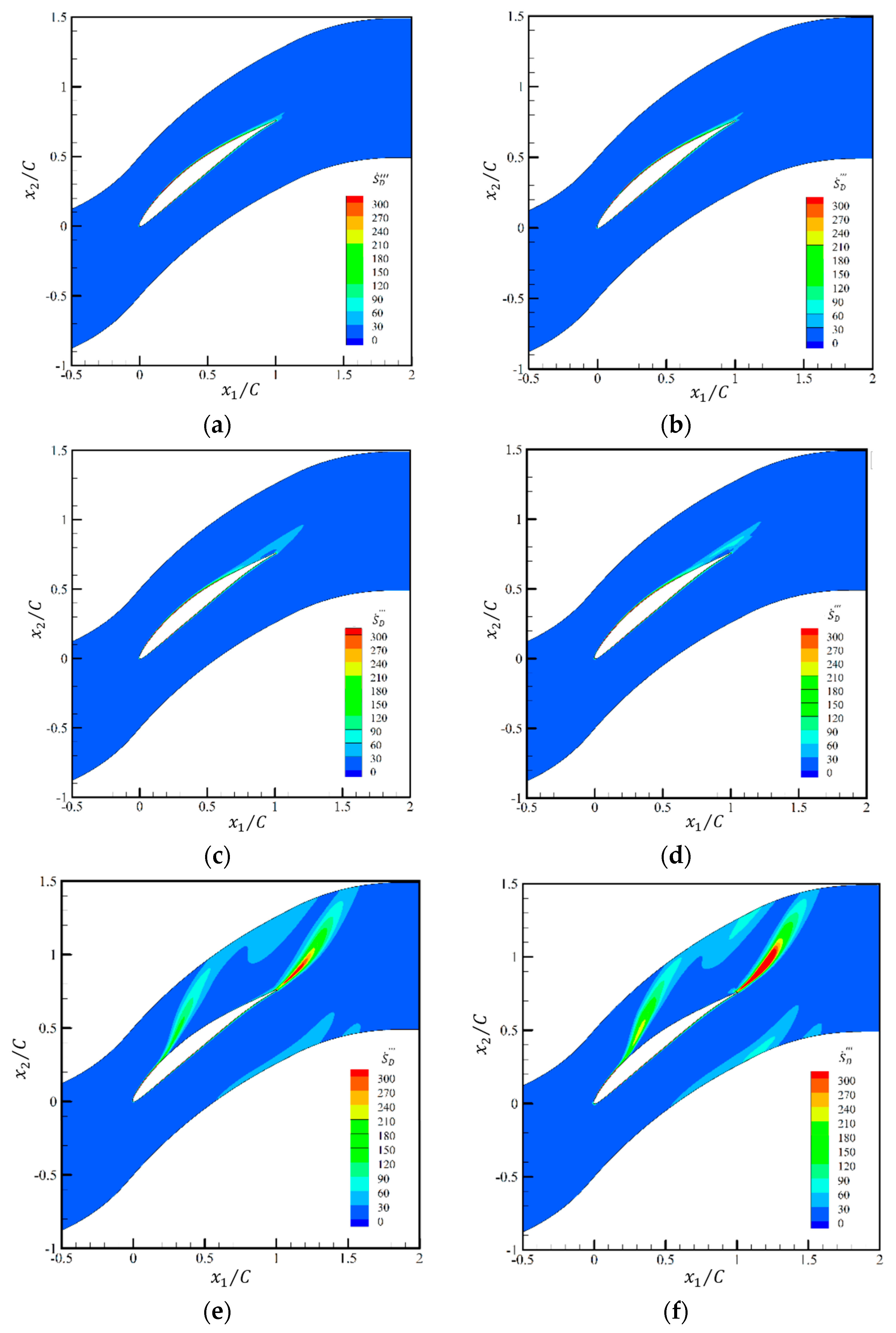
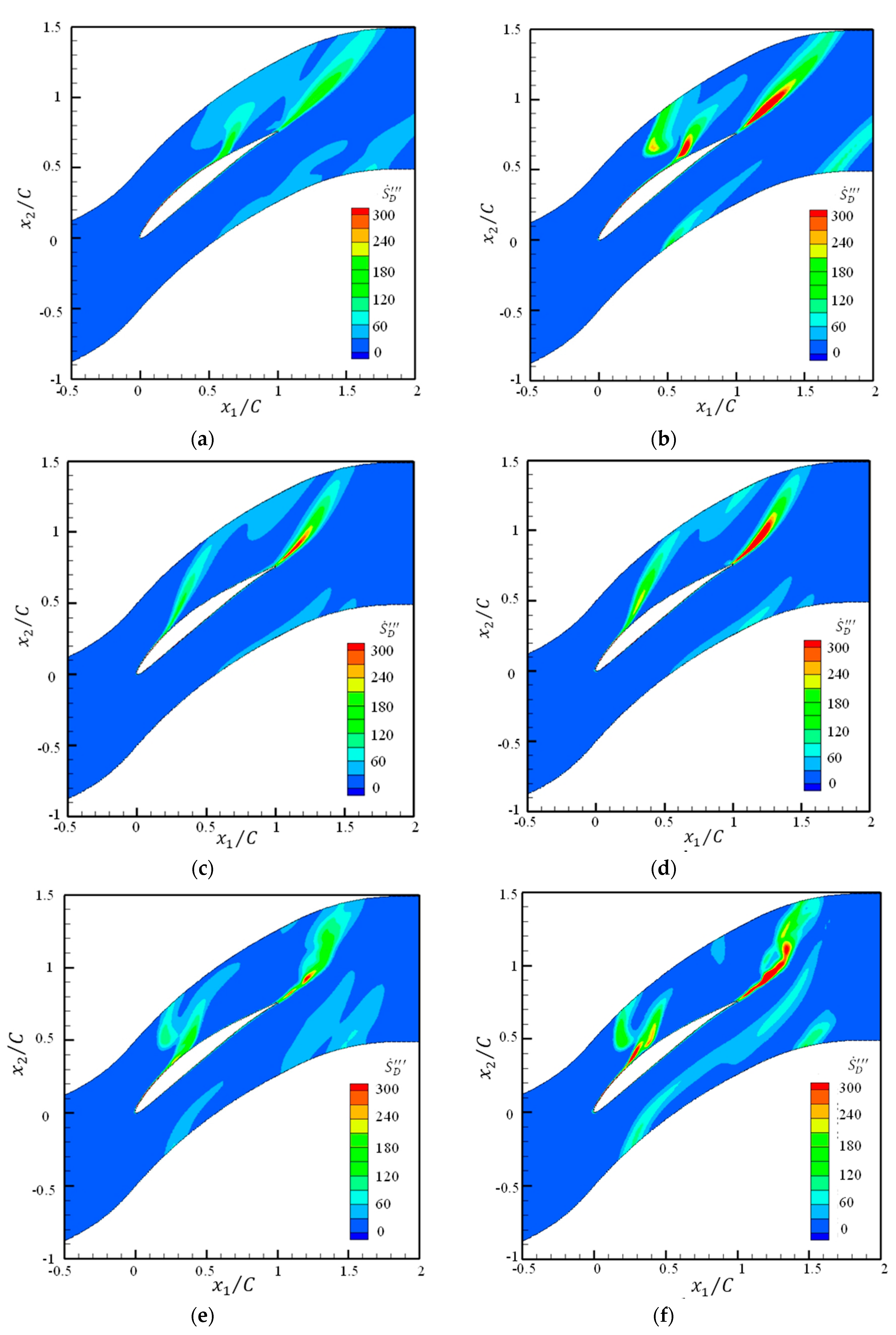
Both model results at the incidence angle of 4° are shown in Figure 5, which indicates that the two models predict similar patterns of entropy generation. close to the hub is stronger according to Equation (35) (see Figure 5f) than Equation (31) (see Figure 5e), since the turbulence production is stronger than the turbulence dissipation in this region. In other words, not all of the produced turbulence is dissipated locally. Similar phenomena can be found at other incidence angles: see Figure 6. However, according to our assumption, the turbulence production is in balance with the turbulence dissipation when the domain size is sufficiently large. This assumption was validated by our numerical results: the volume-integrated entropy generation rates by Equations (31) and (35) can be found in Table 2, which are almost identical. Compared with Equation (31), Equation (35) is more general and is independent of turbulence models.
In the current test case, we are only able to compare the entropy generation rate in the flow field since the energy equation was not solved. More systematic studies, e.g., cascade flows at high Mach numbers, are still required to validate the equivalence between Equation (32) and Equation (36). Besides the entropy generation rates, the other integral quantities for calculating the dimensionless coefficients are also provided in Table 2.
Fluid properties in the combustion chamber, including the specific combustion heat , the heat capacity , and the environmental temperature , are required to determine the local exergy transformation number , which is defined by Equation (24). The values of these parameters are shown in Table 3.
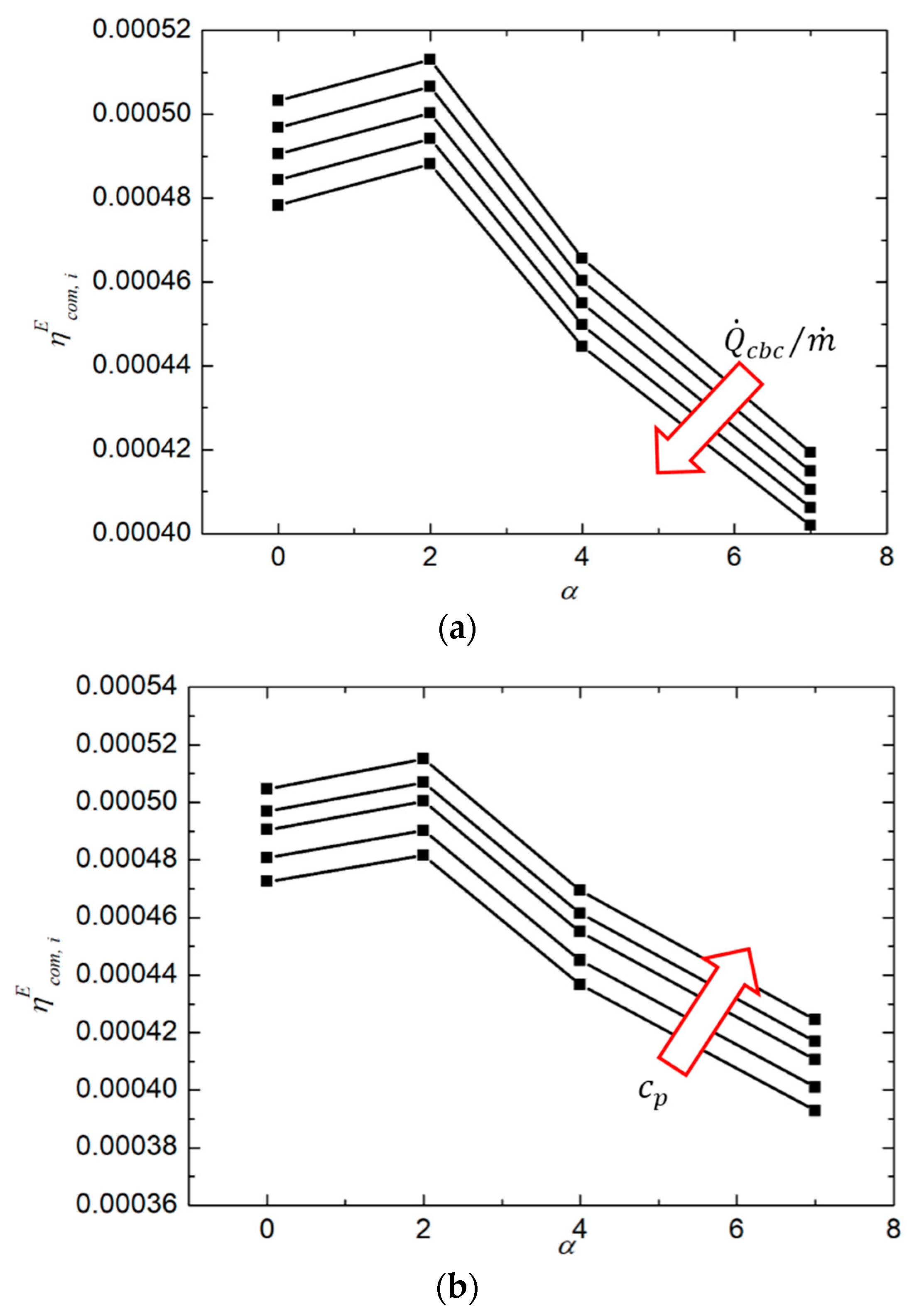
The global coefficients , , and according to the RANS results are shown in Table 4. Both the total pressure loss coefficient and the entropy loss coefficient indicate that losses in the cascade increase with the incidence angle. However, the exergy transformation coefficient suggests that the optimal incidence angle is , at which cascade works with the best overall performance: although more losses due to irreversibility occur at than at , a larger pressure ratio is obtained through the cascade, which increases the potential exergy obtained in the combustion chamber .
The exergy transformation number is linearly related with the environmental temperature , thus does not influence the optimal results. Figure 7 shows the influence of the other reference parameters and on : decreases with and increases with . However, the optimal results are not influenced by and when they are only mildly changed.
6. Conclusions
Several fundamental aspects with respect to the SLA of the turbulent flows in gas turbines were discussed in this study.
Entropy and exergy equations (Equations (8) and (11)) for compressible/incompressible flows in a rotating/non-rotating frame were derived. The derivation shows that the Navier–Stokes equations and the energy equation are sufficient to satisfy the second law of thermodynamics, thus it is not necessary to solve the entropy and exergy equations to evaluate their quantities. The entropy and exergy can be determined by the post processing of CFD simulations. However, the entropy and exergy equations and their budgets are helpful tools for analyzing the irreversible processes in gas turbines.
The exergy transformation efficiency of a gas turbine as well as the exergy transformation number of a single process step were proposed in this study. in a turbine cascade, a compressor cascade, or the combustion chamber are suggested to be calculated by Equations (23), (24), or (28). The value of indicates the overall effects of an irreversible process, including its destruction of exergy and its contribution to the potential exergy obtained in the combustion chamber. can be used to assess the performance of an isolated process in a gas turbine, since only local flow and temperature fields are required to calculate its value.
The methods for calculating the local entropy generation rate densities were discussed. It was suggested to use turbulence production rates (Equations (35) and (36)) instead of the turbulence dissipation rates (Equations (31) and (32)) to calculate the local entropy generation rate densities. The assumption behind this approximation is that the turbulence production rate is in balance with the turbulence dissipation rate when the domain is sufficiently large. An advantage of Equations (35) and (36) is that they are independent from the choices of turbulence models. However, more systematic studies, e.g., LESs of cascade flows at high Mach numbers, are still required to further validate these equations.
A test case with respect to a compressor cascade has been employed for applying the concepts developed in the study. The numerical results show that the entropy generation rates calculated by Equations (35) and (31) are almost identical. The exergy transformation number suggests an optimal incidence angle at which the compressor cascade works with the best overall performance.
Acknowledgments
The authors gratefully acknowledge the support of this study by the DFG-Heisenberg program (JI 253/1) and the grants of National Natural Science Foundation of China (No. 51676184 and No. 51506195). The acknowledgement is also given to X. Ottavy of Ecole Centrale de Lyon for the data support of our test case and H. Herwig of Hamburg University of Technology for the helpful discussion with him.
Author Contributions
Yan Jin proposed the models and derived the mathematical equations. Juan Du, Zhiyuan Li, and Hongwu Zhang performed the CFD simulation. Juan Du and Yan Jin wrote the paper together. Juan Du, Hongwu Zhang, and Yan Jin had deep discussion about the model and the numerical results. All authors have read and approved the final manuscript.
Conflicts of Interest
The authors declare no conflict of interest.
Nomenclature
| local specific internal energy, J kg−1 | |
| local specific exergy of the fluid, J kg−1 | |
| local relative total energy, J kg−1 | |
| body acceleration rate component, m s−2 | |
| body acceleration rate vector, m s−2 | |
| bulk specific primary energy rate, J kg−1 s−1 | |
| local specific enthalpy, J kg−1 | |
| local specific exergy of a gas in an open system, J kg−1 | |
| local kinetic energy, m2 s−2 | |
| inlet specific turbulent kinetic energy, m2 s−2 | |
| mass flow rate, kg s−1 | |
| direction vector of a surface element | |
| length of the blade span, m | |
| energy devaluation number of process step i | |
| blade number in a cascade | |
| local pressure, N m−2 | |
| bulk pressure, N m−2 | |
| local turbulence production rate, kg m−1 s−3 | |
| local temperature fluctuation production rate, J K m−3 s−1 | |
| heat generation rate in the combustion chamber, J s−1 | |
| heat release rate in a reversible Brayton cycle, J s−1 | |
| heat release rate in an irreversible Brayton cycle, J s−1 | |
| exergy of the heat release rate , J s−1 | |
| exergy of the heat generation rate , J s−1 | |
| contribution of process i to , J s−1 | |
| specific gas constant, J kg−1 K−1 | |
| local specific entropy, J kg−1 K−1 | |
| strain rate tensor, s−1 | |
| bulk specific entropy, J kg−1 K−1 | |
| entropy generation rate density in the flow field, J K−1 m−3 s−1 | |
| entropy generation rate density in the temperature field, J K−1 m−3 s−1 | |
| bulk specific entropy potential rate, J kg−1 K−1 s−1 | |
| bulk temperature, K | |
| local velocity vector, m s−1 | |
| local velocity component, m s−1 | |
| local frame velocity vector, m s−1 | |
| local frame velocity component, m s−1 | |
| shaft power of a rotor, J s−1 | |
| displacement vector, m | |
| coordinate vector component, m | |
| Greek symbols | |
| entropy generational rate in process i, J s−1 K−1 | |
| local turbulence dissipation rate, kg m−1 s−3 | |
| local temperature fluctuation dissipation rate, kg K m−1 s−3 | |
| thermal conductivity, J s−1 m−1 K−1 | |
| dynamic viscosity, kg m−1 s−1 | |
| efficiency of an ideal Brayton cycle | |
| efficiency of a real Brayton cycle | |
| exergy transformation efficiency | |
| exergy transformation number of process step | |
| local temperature | |
| viscous stress tensor, k gm−1 s−2 | |
| angular velocity vector, s−1 | |
| inlet specific dissipation rate in the k- SST turbulence model, s−1 | |
| enthalpy loss coefficient | |
| stagnation pressure loss coefficient | |
| entropy loss coefficient | |
| Subscripts | |
| four states of an ideal Brayton cycle | |
| cross section | |
| blade number in a cascade | |
| combustion chamber | |
| compressor | |
| temperature field | |
| flow field | |
| process step index or vector component index | |
| inlet | |
| isentropic value | |
| vector component index | |
| outlet | |
| relative value | |
| total value | |
| turbulence | |
| turbine | |
| wall surface | |
| environmental value | |
| Superscripts | |
| exergy | |
| entropy | |
| * | stagnation value |
| ‘ | irreversible process |
| Reynolds averaging | |
References
- Wang, H. Experimental and Numerical Research of Highly Loaded Axial-Flow Compressor Stages. Ph.D. Thesis, Beihang University, Beijing, China, 2009. [Google Scholar]
- Gao, F. Advanced Numerical Simulation of Corner Separation in a Linear Compressor Cascade. Ph.D. Thesis, Ecole Centrale de Lyon, Écully, France, 2014. [Google Scholar]
- Satoshi, H.; Tsukagoshi, K.; Masada, J.; Ito, E. Test Results of the World’s First 1,600C J-series Gas Turbine. Mitsubishi Heavy Ind. Tech. Rev. 2012, 49, 18–23. [Google Scholar]
- Batchelor, G.K. An Introduction to Fluid Dynamics; Cambridge Mathematical Library: Cambridge, UK, 2000. [Google Scholar]
- Incropera, F.; DeWitt, D.; Bergmann, T.; Lavine, A. Fundamentals of Heat and Mass Transfer, 6th ed.; John Wiley & Sons: New York, NY, USA, 2006. [Google Scholar]
- Bejan, A. Entropy Generation through Heat and Fluid Flow; John Wiley & Sons: New York, NY, USA, 1982. [Google Scholar]
- Bejan, A. Entropy Generation Minimization; CRC Press: Boca Raton, FL, USA, 1996. [Google Scholar]
- Kock, F.; Herwig, H. Local entropy production in turbulent shear flows: A high-Reynolds number model with wall functions. Int. J. Heat Mass Trans. 2004, 47, 2205–2215. [Google Scholar] [CrossRef]
- Kock, F.; Herwig, H. Entropy production calculation for turbulent shear flows and their implementation in CFD codes. Int. J. Heat Fluid Flow 2005, 26, 672–680. [Google Scholar] [CrossRef]
- Jin, Y.; Herwig, H. Turbulent flow in rough wall channels: Validation of RANS models. Comp. Fluids 2015, 122, 34–46. [Google Scholar] [CrossRef]
- Orhan, O.E. Investigation of the Effect of Turbulence on Entropy Generation in Turbomachinery. Ph.D. Thesis, Middle East Technical University, Ankara, Turkey, 2014. [Google Scholar]
- Denton, J.; Pullan, G. A numerical investigation into the sources of endwall loss in axial flow turbines. In Proceedings of the ASME Turbo Expo 2012: Turbine Technical Conference and Exposition, Copenhagen, Denmark, 11–15 June 2012; pp. 1417–1430. [Google Scholar]
- Zlatinov, M.B.; Tan, C.S.; Montgomery, M.; Islam, T.; Harris, M. Turbine hub and shroud sealing flow loss mechanisms. J. Turbomach. 2012, 134, 061027. [Google Scholar] [CrossRef]
- Kopriva, J.E.; Laskowski, G.M.; Sheikhi, M.R.H. Computational assessment of inlet turbulence on boundary layer development and momentum/thermal wakes for high pressure turbine nozzle and blade. In Proceedings of the ASME 2014 International Mechanical Engineering Congress and Exposition, Montreal, QC, Canada, 14–20 November 2014. [Google Scholar]
- Laskowski, G.M.; Kopriva, J.; Michelassi, V.; Shankaran, S.; Paliath, U.; Bhaskaran, R.; Wang, Q.; Talnikar, C.; Wang, Z.; Jia, F. Future directions of high-fidelity CFD for aero-thermal turbomachinery research, analysis and design. In Proceedings of the 46th AIAA Fluid Dynamics Conference, Washington, DC, USA, 13–17 June 2016. [Google Scholar]
- Tucker, P.G. Computation of unsteady turbomachinery flows: Part 1—Progress and challenges. Prog. Aerosp. Sci. 2011, 47, 522–545. [Google Scholar] [CrossRef]
- Tucker, P.G. Computation of unsteady turbomachinery flows: Part 2—LES and hybrids. Prog. Aerosp. Sci. 2011, 47, 546–569. [Google Scholar] [CrossRef]
- Lin, D.; Yuan, X.; Su, X.R. Local Entropy generation in compressible flow through a high pressure turbine with delayed detached eddy simulation. Entropy 2017, 19, 29. [Google Scholar] [CrossRef]
- Wang, H.; Lin, D.; Su, X.R.; Yuan, X. Entropy analysis of the interaction between the corner separation and wakes in a compressor cascade. Entropy 2017, 19, 324. [Google Scholar] [CrossRef]
- ANSYS FLUENT 13.0 User’s Guide, ANSYS Inc.: Canonsburg, PA, USA, 2010.
- Cariglino, F. External Aerodynamic Simulations in a rotating Frame of Reference. Ph.D. Thesis, Politecnico di Torino, Turin, Italy, 2013. [Google Scholar]
- Brown, L. Axial flow compressor and turbine loss coefficients: A comparison of several parameters. J. Eng. Power 1972, 94, 193–201. [Google Scholar] [CrossRef]
- Denton, J.D. Loss mechanisms in turbomachines. In Proceedings of the ASME 1993 International GasTurbine and Aeroengine Congress and Exposition, Cincinnati, OH, USA, 24–27 May 1993. [Google Scholar]
- Redecker, C.; Herwig, H. Calculating and assessing complex convective heat transfer problems: The CFD-SLA approach. In Proceedings of the 15th International Heat Transfer Conference, Kyoto, Japan, 10–15 August 2014. [Google Scholar]
- Wenterodt, T.; Redecker, C.; Herwig, H. Second law analysis for sustainable heat and energy transfer: The entropic potential concept. Appl. Energy 2015, 139, 376–383. [Google Scholar] [CrossRef]
- Herwig, H.; Redecker, C. Heat transfer and entropy. In Heat Transfer Studies and Applications; Kazi, S.N., Ed.; InTech: Rijeka, Croatia, 2015; pp. 143–161. [Google Scholar]
- Pope, S.B. Turbulent Flows; Cambridge University Press: Cambridge, UK, 2000. [Google Scholar]
- Ma, W. Experimental Investigation of Corner Stall in a Linear Compressor Cascade. Ph.D. Thesis, Ecole Centrale de Lyon, Écully, France, 2012. [Google Scholar]
- Menter, F.R. Two equation Eddy viscosity turbulence models for engineering applications. AIAA J. 1994, 32, 1598–1605. [Google Scholar] [CrossRef]
- Li, Z.Y.; Du, J.; Jemcov, A.; Ottavy, X.; Lin, F. A study of loss mechanism in a linear compressor cascade at the corner stall condition. In Proceedings of the ASME Turbo Expo 2017: Turbomachinery Technical Conference and Exposition (GT2017), Charlotte, NC, USA, 26–30 June 2017. [Google Scholar]
Figure 1.
The schematic diagram of ideal (0–1–2–3–0) and real (0–1’–2’–3’–0) Brayton cycles in a gas turbine. (a) The temperature–entropy diagram; (b) The schematic diagram of a gas turbine. The hot air at 3(3’) cools down in the atmosphere to become cold air at 0. Only the irreversible processes in the compressor (0–1’) and the turbine (2’–3’) are under consideration.

Figure 2.
Influence of compressor cascade i on the exergy obtained in the combustion chamber. (a) A gas turbine with i − 1 compressor cascades: the inlet and outlet temperature of the combustion chamber is and ; (b) A gas turbine with i compressor cascades: the inlet and outlet temperature of the combustion chamber is and . The static temperature is increased from to through compressor cascade i.
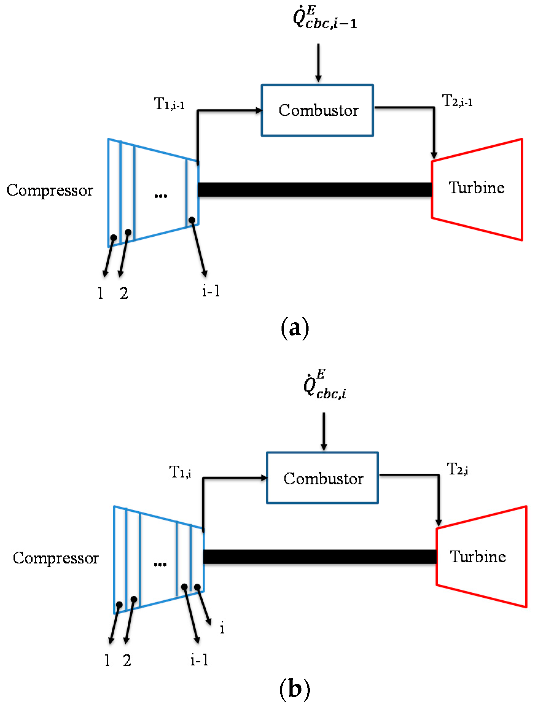
Figure 3.
The computational domain and the mesh resolution in a cross section.

Figure 4.
The static pressure coefficient (Cp) on the blade wall surface; comparison between the current computational fluid dynamics (CFD) results and the experimental data in [28]. (a) ; (b) .
Figure 4.
The static pressure coefficient (Cp) on the blade wall surface; comparison between the current computational fluid dynamics (CFD) results and the experimental data in [28]. (a) ; (b) .
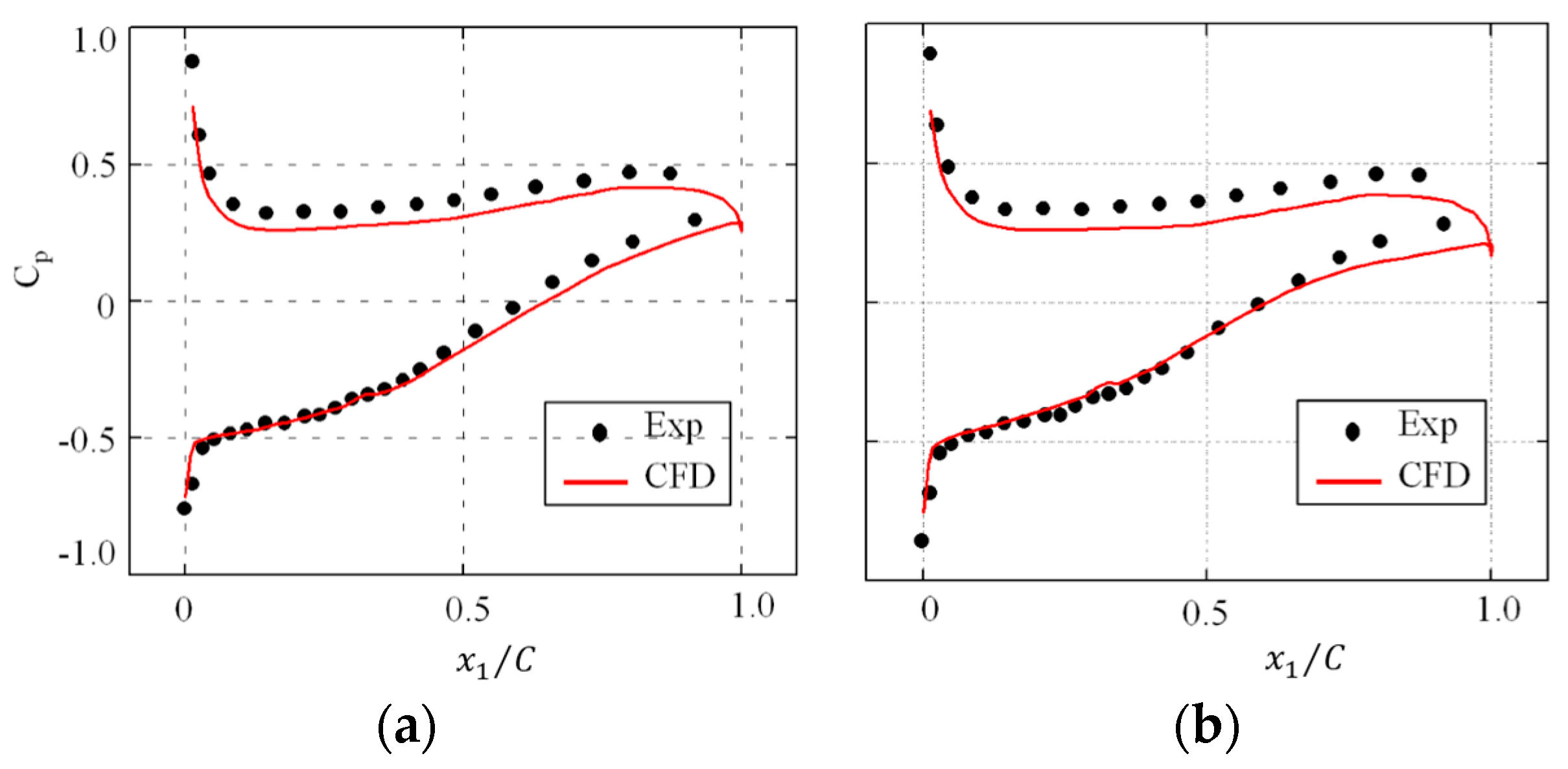
Figure 5.
The distribution of the entropy production rate density at different cross sections. The incidence angle is 4°. (a) Equation (31), = 50% (mid-plane); (b) Equation (35), = 50% (mid-plane); (c) Equation (31), = 25%; (d) Equation (35), = 25%; (e) Equation (31), = 5% (close to the hub); (f) Equation (35), = 5% (close to the hub).

Figure 6.
The distribution of the entropy production rate in a plane close to the hub ( = 5%) for different incidence angles. (a) α = 2°, Equation (31); (b) α = 2°, Equation (35); (c) α = 4°, Equation (31); (d) α = 4°, Equation (35); (e) α = 7°, Equation (31); (f) α = 7°, Equation (35).
Figure 6.
The distribution of the entropy production rate in a plane close to the hub ( = 5%) for different incidence angles. (a) α = 2°, Equation (31); (b) α = 2°, Equation (35); (c) α = 4°, Equation (31); (d) α = 4°, Equation (35); (e) α = 7°, Equation (31); (f) α = 7°, Equation (35).

Figure 7.
Influence of the reference parameters on the exergy transformation number . (a) varies from J kg−1 to J kg−1; (b) varies from 950 J kg−1 K−1 to 1050 J kg−1 K−1. The arrows indicate the direction of increasing and .
Figure 7.
Influence of the reference parameters on the exergy transformation number . (a) varies from J kg−1 to J kg−1; (b) varies from 950 J kg−1 K−1 to 1050 J kg−1 K−1. The arrows indicate the direction of increasing and .

Table 1.
Geometric parameters of the cascade.
| Parameter | Value |
|---|---|
| Chord (m) | 0.15 |
| Camber angle (°) | 23.22 |
| Stagger angle (°) | 42.7 |
| Pitch spacing (m) | 0.134 |
| Solidity | 1.12 |
| Blade span (m) | 0.37 |
| Aspect ratio | 2.47 |
| Design upstream flow angle (°) | 54.31 |
| Design downstream flow angle (°) | 31.09 |
Table 2.
Time- and volume-averaged dimensional Reynolds Averaged Navier–Stokes (RANS) results. The local entropy generation rate was calculated with Equation (35). is the entropy generation rate in a half-cascade passage, and is the entropy generation rate in a cascade.
Table 2.
Time- and volume-averaged dimensional Reynolds Averaged Navier–Stokes (RANS) results. The local entropy generation rate was calculated with Equation (35). is the entropy generation rate in a half-cascade passage, and is the entropy generation rate in a cascade.
| Bulk Variables | ||||
|---|---|---|---|---|
| (W K−1) (Equation (31)) | 0.0705 | 0.0795 | 0.0976 | 0.108 |
| (W K−1) (Equation (35)) | 0.0695 | 0.0782 | 0.101 | 0.112 |
| (kg s−1) | 0.6897 | 0.656 | 0.621 | 0.568 |
| (Pa) | 101,009 | 100,996 | 101,004 | 101,015 |
| (Pa) | 101,955 | 101,941 | 101,949 | 101,960 |
| (K) | 296.94 | 296.90 | 296.93 | 296.96 |
| (K) | 299.72 | 299.68 | 299.71 | 299.74 |
| (Pa) | 101,325 | 101,325 | 101,325 | 101,325 |
| (Pa) | 101,922 | 101,896 | 101,886 | 101,888 |
| (K) | 297.87 | 297.87 | 297.87 | 298.87 |
| (K) | 299.53 | 299.55 | 299.52 | 299.53 |
Table 3.
The reference parameters for calculating the local exergy transformation number . and are the properties of the gas in the combustion chamber.
Table 3.
The reference parameters for calculating the local exergy transformation number . and are the properties of the gas in the combustion chamber.
| Parameters | Values |
|---|---|
| (K) | 288.15 |
| (J kg−1) | |
| (J kg−1 K−1) | 1005 |
Table 4.
Global coefficients according to the RANS results. The local entropy generation rate was calculated with Equation (35). The optimal exergy transformation number is shown with grey background.
Table 4.
Global coefficients according to the RANS results. The local entropy generation rate was calculated with Equation (35). The optimal exergy transformation number is shown with grey background.
| Dimensionless Coefficients | ||||
|---|---|---|---|---|
| (Equation (15)) | 0.0349 | 0.0476 | 0.0667 | 0.0762 |
| (Equation (16)) | 0.0107 | 0.0127 | 0.0173 | 0.0210 |
| (Equation (24)) | 0.000490 | 0.000500 | 0.000455 | 0.000411 |
© 2017 by the authors. Licensee MDPI, Basel, Switzerland. This article is an open access article distributed under the terms and conditions of the Creative Commons Attribution (CC BY) license (http://creativecommons.org/licenses/by/4.0/).
Share and Cite
MDPI and ACS Style
Jin, Y.; Du, J.; Li, Z.; Zhang, H. Second-Law Analysis of Irreversible Losses in Gas Turbines. Entropy 2017, 19, 470. https://doi.org/10.3390/e19090470
AMA Style
Jin Y, Du J, Li Z, Zhang H. Second-Law Analysis of Irreversible Losses in Gas Turbines. Entropy. 2017; 19(9):470. https://doi.org/10.3390/e19090470
Chicago/Turabian StyleJin, Yan, Juan Du, Zhiyuan Li, and Hongwu Zhang. 2017. "Second-Law Analysis of Irreversible Losses in Gas Turbines" Entropy 19, no. 9: 470. https://doi.org/10.3390/e19090470
Note that from the first issue of 2016, this journal uses article numbers instead of page numbers. See further details here.