Article

Coupled Effects of Turing and Neimark-Sacker Bifurcations on Vegetation Pattern Self-Organization in a Discrete Vegetation-Sand Model

Research Center for Engineering Ecology and Nonlinear Science, North China Electric Power University, Beijing 102206, China
*
Author to whom correspondence should be addressed.
Entropy 2017, 19(9), 478; https://doi.org/10.3390/e19090478
Submission received: 12 July 2017 / Revised: 11 August 2017 / Accepted: 4 September 2017 / Published: 8 September 2017
(This article belongs to the Special Issue Complex Systems, Non-Equilibrium Dynamics and Self-Organisation)

Abstract

:
Wind-induced vegetation patterns were proposed a long time ago but only recently a dynamic vegetation-sand relationship has been established. In this research, we transformed the continuous vegetation-sand model into a discrete model. Fixed points and stability analyses were then studied. Bifurcation analyses are done around the fixed point, including Neimark-Sacker and Turing bifurcation. Then we simulated the parameter space for both bifurcations. Based on the bifurcation conditions, simulations are carried out around the bifurcation point. Simulation results showed that Neimark-Sacker bifurcation and Turing bifurcation can induce the self-organization of complex vegetation patterns, among which labyrinth and striped patterns are the key results that can be presented by the continuous model. Under the coupled effects of the two bifurcations, simulation results show that vegetation patterns can also be self-organized, but vegetation type changed. The type of the patterns can be Turing type, Neimark-Sacker type, or some other special type. The difference may depend on the relative intensity of each bifurcation. The calculation of entropy may help understand the variance of pattern types.

1. Introduction

Vegetation patterns have been widely observed in arid and semi-arid areas [1,2,3,4,5,6,7]. There have been many studies on the exploration of pattern self-organization mechanisms [8,9,10,11,12,13]. This research has contributed to the understanding of vegetation competition when resources are limited and the process by which robust land is converted into desert because of climate change or anthropogenic disturbances [14,15]. The relationship between self-organization and the production of entropy can find its origin in the pioneering works in [16,17]. Since then many studies have explored the relationship in a variety of fields [18,19]. The calculation of entropy can be used for pattern classification [20], therefore, the investigation of the mechanisms of self-organization will enhance the understanding of entropy. Besides, due to the complexity of the ecological scale, investigation of vegetation patterns has never stopped.
Vegetation bands lying perpendicular to the prevailing wind direction have been observed, showing dying trees in the windward edge and seedling regrowth on the leeward edge of each band [21,22,23]. While [24,25] suggested that in Jordan wind might be the initiating and driving factor of banded patterns and the accumulation of wind-blown material around isolated plants might act as a nucleus for the development of vegetation arcs. Dynamical models for these wind-induced vegetation patterns have been rare. Recently Zhang et al. [26] proposed a vegetation-sand model using partial differential equations to interpret the mechanism of vegetation self-organization in windy sandy environments [27,28,29,30,31]. In the model of Zhang et al. [26], wind is considered as prevailing and non-prevailing (defined as winds from all other directions except the prevailing wind direction) and each has different effects on vegetation dispersal and sand transportation. The effects of prevailing wind on sand and vegetation are modeled by advection terms, while the effects of non-prevailing wind are modeled as diffusion terms. Simulations showed that without the prevailing wind labyrinth vegetation patterns can be obtained, and with the prevailing wind banded vegetation patterns perpendicular to the prevailing wind direction can be obtained.
In Nature, wind events and sand movements are discrete. Wind collection and recording are also discrete. Therefore, we think the discretization of the continuous model is necessary. Discrete models have provided advantages in revealing complex nonlinear dynamics. A classic example is the discrete logistic model that exhibits period-doubling cascade and a route to chaos [32]. In contrast, the continuous logistic model provides a simple “S” form curve, and never demonstrates the above dynamic complexity. Through a variety of bifurcations, discrete models can generate periodic orbits, invariant circles, periodic windows, chaotic behavior and so on. More importantly, as births and deaths of bionts in predator-prey systems are discrete events, continuous models only make sense for very large populations. Other researchers propose that discrete models reveal the discontinuous properties (such as a patchy environment or a fragmented habitat) of predator-prey systems [33]. Discrete models may exhibit new dynamical behaviors. For example, Han et al. found that Turing instability and Turing patterns can occur in a simple discrete competitive Lotka-Volterra system rather than a continuous one [34].
In the discrete model, focusing on the time scale, Neimark-Sacker bifurcation can occur without spatial terms. Neimark-Sacker bifurcation is one of the most important bifurcations in discrete dynamics. Through Neimark-Sacker bifurcation, a system stable states bifurcate from a fixed point to an invariant circle. It should be noted that with spatial terms such as advection and diffusion, Turing bifurcation can also occur. Naturally, a question arises as to what the dynamics will be when Turing and Neimark-Sacker bifurcation occur at the same time, and how they influence the self-organization of vegetation patterns. To the authors’ knowledge, there have been no simulations of the coupling effects of Turing and Neimark-Sacker bifurcations on vegetation patterns.
In this research, we will transform the vegetation-sand model [26] to a spatially and temporally discrete model. Then, focusing on the stable fixed point, bifurcation analysis including Neimark-Sacker bifurcation and Turing bifurcation will be carried out. Bifurcation diagram and phase portrait will be shown. Based on bifurcation analysis, parameter values will be selected around each bifurcation. Given these parameters, simulations will be carried out to show how patterns transform from Turing bifurcation to Turing-Neimark-Sacker bifurcation (Turing bifurcation and Neimark-Sacker bifurcation occur at the same time). Different transformation processes will be simulated. Finally, we will discuss the possible reason that cause the different transformations.

2. A Discrete Vegetation-Sand Model

The continuous vegetation-sand model was proposed by [26] and is shown as:
S t = k 0 + m V ( 1 V V 0 ) n S a 1 S x + D 1 ( 2 S x 2 + 2 S y 2 ) , V t = h V ( 1 V V m ) p S V C + V a 2 V x + D 2 ( 2 V x 2 + 2 V y 2 )
The model is considered in the dimensional form rather than the non-dimensional form. This is because there are few parameters, and each parameter has its own ecological significance. Here S (cm) represents the height of sand deposition. Parameter k0 (cm·d−1) is the accumulation rate of air sand without vegetation. m (cm·d−1) is the coefficient representing the trapping effect of vegetation. Parameters k0 and m are affected by sand flow intensity. The trapping effects of vegetation decrease with the increase of vegetation cover until a certain value (near 100%) of vegetation cover (saturation constant of vegetation trapping effects), and V0 (%) is two times of this certain value. n (d−1) is the coefficient representing the decrease of accumulation rate with the increase of sand height. a1 (m·d−1) is the coefficient representing the translation of sand dunes by wind. D1 (m2·d−1) is the diffusion coefficient of sand without strong unidirectional wind. V (%) represents vegetation coverage, and h (d−1) represents the intrinsic growth rate of vegetation. Vm (%) is the potential maximum of vegetation coverage. p (cm−1·d−1) is the coefficient of destruction effect by sand. C (%) is a constant representing how sand tolerance increases with the increase of vegetation cover. a2 (m·d−1) is the advection coefficient representing the dispersal of vegetation by wind. D2 (m2·d−1) is the diffusion coefficient representing the dispersal of vegetation without strong unidirectional wind. x and y are space axes, and t is time. Wind direction is along the positive x direction. When there is no prevailing wind, the effects of wind are modeled as diffusion terms. When there is a prevailing wind, its effects can be modeled by adding an advection term to the diffusion term as shown in Equation (1).
In this research, the above continuous model will be transformed to a discrete model (Equation (2)). We consider the model on a N × N lattice, and the two variables can be expressed as S(i,j,t) and V(i,j,t) (i,j ∈ {1, 2, 3, …, N} and tZ+), that represent the height of sand deposition and the vegetation coverage in lattice (i,j) at time t, respectively. According to the former research works of [33,35,36,37], there are two stages, reaction stage and diffusion stage, when we discretize the continuous model (Equation (1)). The spatial dispersal stage, that are advection and diffusion, is considered firstly as:
{ S ( i , j , t ) = S ( i , j , t ) + τ d a 1 d S ( i , j , t ) + τ d 2 D 1 d 2 S ( i , j , t ) V ( i , j , t ) = V ( i , j , t ) + τ d a 2 d V ( i , j , t ) + τ d 2 D 2 d 2 V ( i , j , t ) .
where S(i,j,t) and V(i,j,t) are the transitional variables of S and V after one step of dispersal stage. τ (days) and d (meters) are the time step and space step respectively. d denotes the discrete form of advections. d 2 denotes the discrete form of the Laplacian operator:
d S ( i , j , t ) = S ( i + 1 , j , t ) S ( i , j , t ) d V ( i , j , t ) = V ( i + 1 , j , t ) V ( i , j , t ) d 2 S ( i , j , t ) = S ( i + 1 , j , t ) + S ( i 1 , j , t ) + S ( i , j + 1 , t ) + S ( i , j 1 , t ) 4 S ( i , j , t ) d 2 V ( i , j , t ) = V ( i + 1 , j , t ) + V ( i 1 , j , t ) + V ( i , j + 1 , t ) + V ( i , j 1 , t ) 4 V ( i , j , t ) .
Boundary conditions are set as periodic conditions. Then we consider the reaction stage:
{ S ( i , j , t + 1 ) = f 1 ( S ( i , j , t ) , V ( i , j , t ) ) = S ( i , j , t ) + τ f ( S ( i , j , t ) , V ( i , j , t ) ) V ( i , j , t + 1 ) = g 1 ( S ( i , j , t ) , V ( i , j , t ) ) = V ( i , j , t ) + τ g ( S ( i , j , t ) , V ( i , j , t ) ) ,
in which:
{ f ( S , V ) = k 0 + m V ( 1 V V 0 ) n S g ( S , V ) = h V ( 1 V V m ) p S V C + V ,
Equations (2) and (4) including both diffusion and reaction stages are defined as our discrete model.
As the previous work in [26] has been done on the condition of equilibrium in the continuous model, we focus on one of the most important situations, which has three equilibria under the same parameter condition. The three equilibria are: one boundary equilibrium (Sb,Vb), one unstable saddle point (S2,V2), and one locally asymptotical stable node (S1,V1). These equilibria are also fixed points in the discrete model, and can be expressed as:
( S b , V b ) = ( k 0 n , 0 ) ,
( S 1 , V 1 ) = ( k 0 n + m b 4 n ( 1 b 4 V 0 ) , b 4 ) ,
( S 2 , V 2 ) = ( k 0 n + m b 5 n ( 1 b 5 V 0 ) , b 5 ) ,
in which:
b 1 = ( h p V m m n V 0 ) , b 2 = ( m n h p + h C p V m ) , b 3 = ( k 0 n h C p ) , b 4 = b 2 + b 2 2 4 b 1 b 3 2 b 1 , b 5 = b 2 b 2 2 4 b 1 b 3 2 b 1 ,
In [26], stability analysis shows that (S1,V1) is the only locally asymptotically stable interior equilibrium. Therefore focusing on (S1,V1), we have the Jacobian matrix:
J ( S , V ) = ( 1 n τ τ m ( 2 V + V 0 ) V 0 τ p V C + V 1 + τ ( h 2 h V V m p S C ( C + V ) 2 ) ) ,
and eigenvalues:
λ 1 , 2 = t r 0 ± t r 0 2 4 Δ 0 2
In which (S1,V1) is the interior fixed point, and:
t r 0 = 2 τ ( n h + 2 h V 1 V m + p S 1 C ( C + V 1 ) 2 ) Δ 0 = 1 + τ ( h n 2 h V 1 V m p S 1 C ( C + V 1 ) 2 ) + τ 2 ( n h + 2 n h V 1 V m + n p S 1 C ( C + V 1 ) 2 + m p V 1 ( 2 V 1 + V 0 ) ( C + V 1 ) V 0 ) .
Therefore (S1,V1) is locally asymptotically stable only when|λ1| < 1, and |λ2| < 1, which yields:
{ Δ 0 < 1 ( 1 + Δ 0 ) < t r 0 < 1 + Δ 0 ,
We set most parameter values unchanged in this research: h = 0.2 d−1; Vm = 100%; p = 0.045 cm−1·d−1; m = 0.2 cm·d−1; n = 0.07 d−1; V0 = 200%; C = 10%; D2 = 0.01 m2·d−1. And other parameters such as k0, D1, a2, a1, τ and h1 will vary.

3. Bifurcation Analysis

Turing bifurcation is most commonly used in the study of vegetation self-organized patterns, and there are many studies focusing on Turing type patterns [38,39,40]. Spatial symmetry breaking can be induced by Turing bifurcation, leading to the formation of patterns that are stationary in time and oscillatory in space. While there is another type of symmetry breaking, temporal symmetry breaking. Temporal symmetry breaking can be induced by Neimark-Sacker bifurcation, giving rise to states that are homogeneous in space and oscillatory in time. When temporal and spatial symmetry breakings take place simultaneously, the discrete model will generate the patterns that are oscillatory in both space and time. In this section, the parameter conditions of Neimark-Sacker bifurcation, Turing bifurcation and both bifurcations will be obtained. Bifurcation analysis will be focused on the fixed point (S1,V1). The condition of Neimark-Sacker bifurcation will be calculated and bifurcation diagram will be shown. Then Turing bifurcation will be re-investigated as the model has been transformed to a discrete model. And based on the two bifurcation conditions, we choose two key parameters τ and a1 and calculate the parameter space that satisfy both bifurcations. In this section, we will only show the key results of Neimark-Sacker and Turing bifurcation analysis. The complete calculation process of each bifurcation condition can be seen in the Appendix A.

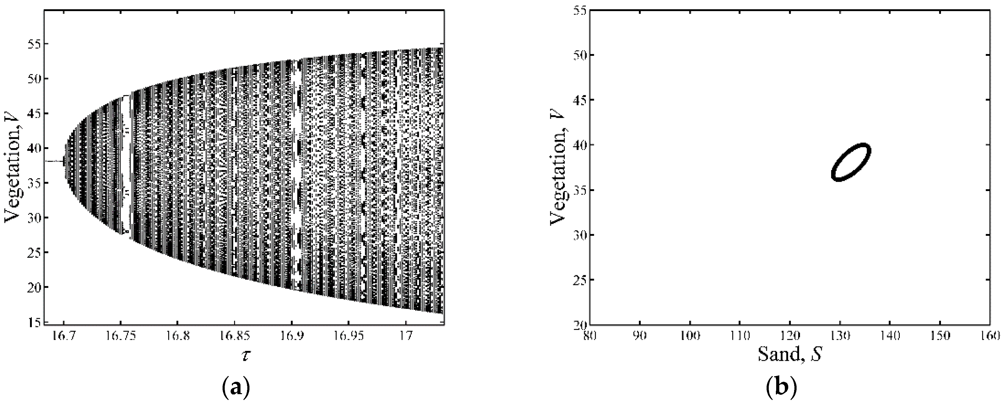
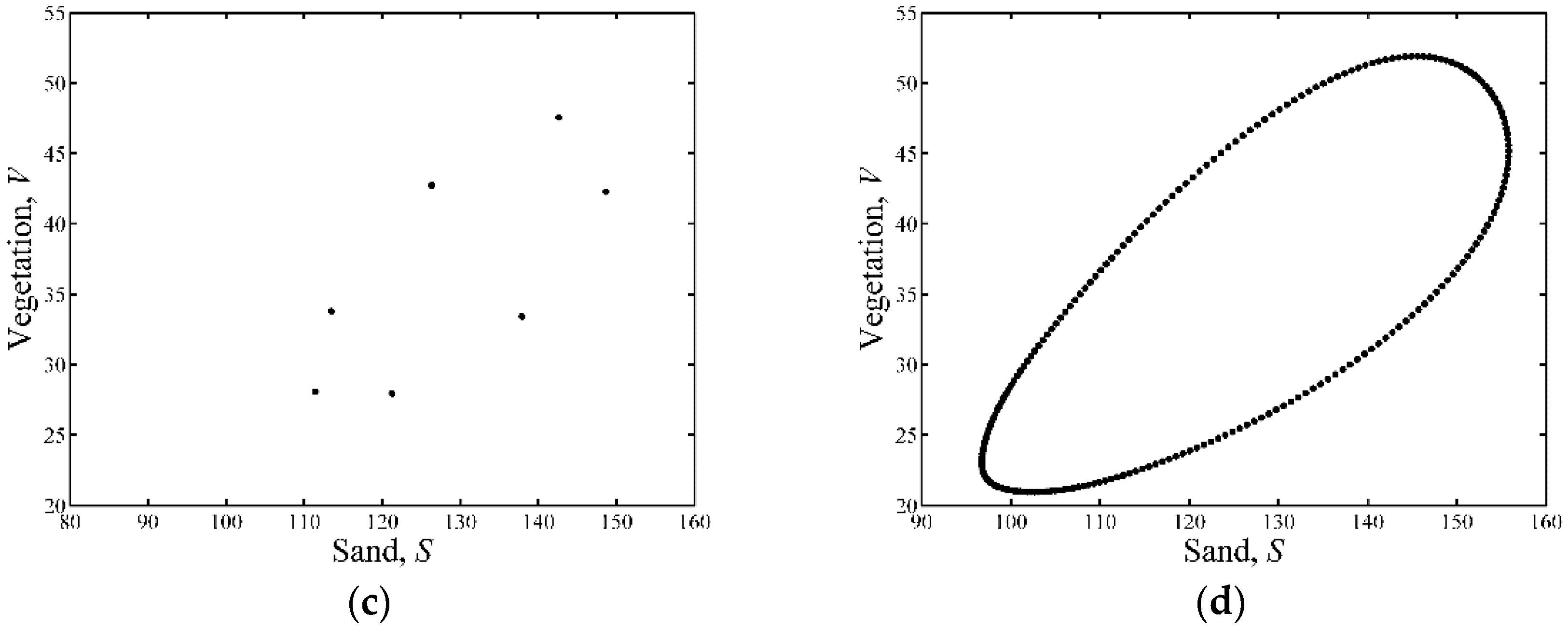
3.1. Neimark-Sacker Bifurcation Analysis

According to [41], assume that U0(μ) is the asymptotically stable fixed points of map:
U 0 F ( U 0 ,   μ ) ,   U 0 R 2 ,   μ R 1
and its eigenvalues are conjugate λ ( μ ) , λ ¯ ( μ ) . If:
| λ ( μ 0 ) | = 1 , λ j ( μ 0 ) 1 ,   j = 1 , 2 , 3 , 4
d d μ ( | λ ( μ 0 ) | ) 0 ,
a = Re ( ( 1 2 λ ¯ ) λ ¯ 2 1 λ ξ 11 ξ 20 ) 1 2 | ξ 11 | 2 | ξ 02 | 2 + Re ( λ ¯ ξ 21 ) 0 ,
in which:
ξ 20 = 1 8 ( ( F x ˜ x ˜ F y ˜ y ˜ + 2 G x ˜ y ˜ ) + i ( G x ˜ x ˜ G y ˜ y ˜ 2 F x ˜ y ˜ ) ) ,
ξ 11 = 1 4 ( ( F x ˜ x ˜ + F y ˜ y ˜ ) + i ( G x ˜ x ˜ + G y ˜ y ˜ ) ) ,
ξ 02 = 1 8 ( ( F x ˜ x ˜ F y ˜ y ˜ 2 G x ˜ y ˜ ) + i ( G x ˜ x ˜ G y ˜ y ˜ + 2 F x ˜ y ˜ ) ) ,
ξ 21 = 1 16 ( ( F x ˜ x ˜ x ˜ + F x ˜ y ˜ y ˜ + G x ˜ x ˜ y ˜ + G y ˜ y ˜ y ˜ ) + i ( G x ˜ x ˜ x ˜ + G x ˜ y ˜ y ˜ F x ˜ x ˜ y ˜ F y ˜ y ˜ y ˜ ) ) .
then the Map (14) undergoes Neimark-Sacker bifurcation when μ = μ0,
Our discrete model can be transformed into a map:
( S V ) ( S + τ ( k 0 + m V ( 1 V V 0 ) n S ) V + τ ( h V ( 1 V V m ) p S V C + V ) )
Considering Map (22), (S1,V1) is also the asymptotically stable fixed point. Then the map undergoes Neimark-Sacker bifurcation at the fixed point (S1,V1), when τ = τ0, in which:
τ 0 = n h + 2 h V 1 V m + p S 1 C ( C + V 1 ) 2 n h + 2 n h V 1 V m + n p S 1 C ( C + V 1 ) 2 + m p V 1 ( 2 V 1 + V 0 ) ( C + V 1 ) V 0
and τ0 satisfies the following conditions:
τ 0 ( n h + 2 h V 1 V m + p S 1 C ( C + V 1 ) 2 ) 2 , 3 .
a = A N M B 32 a 12 2 β 2 ( ( 1 α ) 2 + β 2 ) 1 32 a 12 2 β 2 ( ( G 1 w ˜ w ˜ + G 1 z ˜ z ˜ ) 2 + ( G 2 w ˜ w ˜ + G 2 z ˜ z ˜ ) 2 ) 1 64 a 12 2 β 2 ( ( G 1 w ˜ w ˜ G 1 z ˜ z ˜ 2 G 2 w ˜ z ˜ ) 2 + ( G 2 w ˜ w ˜ G 2 z ˜ z ˜ + 2 G 1 w ˜ z ˜ ) 2 ) + 1 16 a 12 β ( α ( G 2 w ˜ w ˜ z ˜ + G 2 z ˜ z ˜ z ˜ ) + β ( G 2 w ˜ w ˜ w ˜ + G 2 w ˜ z ˜ z ˜ ) ) 0
in which:
M = β ( 3 4 α ) ( α 2 β 2 ) 2 α β ( ( 1 α ) ( 1 2 α ) 2 β 2 ) , N = ( 1 3 α + 2 α 2 2 β 2 ) ( α 2 β 2 ) + ( 6 α 8 α 2 ) β 2 , A = ( G 1 w ˜ w ˜ + G 1 z ˜ z ˜ ) ( G 1 w ˜ w ˜ G 1 z ˜ z ˜ + 2 G 2 w ˜ z ˜ ) ( G 2 w ˜ w ˜ + G 2 z ˜ z ˜ ) ( G 2 w ˜ w ˜ G 2 z ˜ z ˜ 2 G 1 w ˜ z ˜ ) , B = ( G 2 w ˜ w ˜ + G 2 z ˜ z ˜ ) ( G 1 w ˜ w ˜ G 1 z ˜ z ˜ + 2 G 2 w ˜ z ˜ ) + ( G 1 w ˜ w ˜ + G 1 z ˜ z ˜ ) ( G 2 w ˜ w ˜ G 2 z ˜ z ˜ 2 G 1 w ˜ z ˜ ) .
Figure 1 shows the variations of V versus parameter τ when the parameter values satisfy the Neimark-Sacker bifurcation condition. Note that this bifurcation diagram has no visible periodic windows. When τ < 16.6997 days, the fixed point is asymptotically stable. When τ = 16.6997 days, the system starts to bifurcate around a fixed point. As the value of τ increases, the stable states of the system in the phase plane (V,S) experience several stages, such as invariant circle (τ = 16.7013 days as shown in Figure 1b), period-7 (τ = 16.755 days as shown in Figure 1c), and then invariant circle again (τ = 16.8667 days as shown in Figure 1d). Then the stable states of the system may go through several multi-period and invariant circle stages.

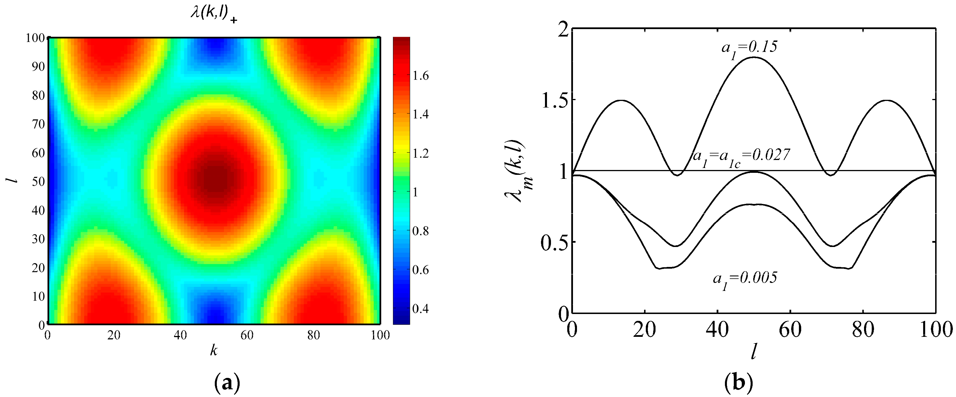
3.2. Turing Bifurcation Analysis

According to [42], assume that U0(μ) is the fixed points of one reaction-diffusion model:
U t + 1 = v 1 f ( U t , μ ) + v 2 d 2 U t + v 3 d U t ,
In which, d and d 2 denotes the discrete form of advection and Laplacian operator respectively. f is smooth. v1, v2, v3 are coefficients. λ(μ) is the eigenvalues of the model at U = U0(μ). When:
  • In the absence of diffusion and advection, U0(μ) is asymptotically stable;
  • With diffusion and advection, max(λ(μ)) > 0;
then the model undergoes Turing bifurcation.
In the discrete models, eigenvalues of d and d 2 are difficult to obtain. But according to the method in [43], the eigenvalues of d can be obtained as:
λ k l 1 = 2 sin ϕ k exp ( ( ϕ k π 2 ) i ) .
where ϕ k = ( k 1 ) π / N , k { 1 , 2 , 3 , , N } and i represents the complex unit, that is i = 1 . While the eigenvalues of d 2 can be obtained as:
λ k l = 4 ( sin 2 ϕ k + sin 2 ϕ l ) ,
in which ϕ k = ( k 1 ) π / N , ϕ l = ( l 1 ) π / N , and k ,   l { 1 , 2 , 3 , , N } .
In this research, we have known that (S1,V1) is the asymptotically stable fixed point of our discrete vegetation-sand model (Equations (2) and (4)). The eigenvalues of the model are:
λ ± ( k , l , τ ) = 1 2 t r ( k , l , τ ) ± 1 2 t r ( k , l , τ ) 2 4 Δ ( k , l , τ ) ,
in which:
t r ( k , l , τ ) = t r 0 ( τ ) + τ d ( a 11 ( τ ) a 1 + a 22 ( τ ) a 2 ) a 1 λ k l 1 + τ d 2 ( a 11 ( τ ) D 1 + a 22 ( τ ) D 2 ) λ k l ,
Δ ( k , l , τ ) = Δ 0 ( τ ) ( 1 + τ d a 1 λ k l 1 D 1 τ d 2 λ k l ) ( 1 + τ d a 2 λ k l 1 τ d 2 D 2 δ λ k l ) .
Here tr0(τ), ∆0(τ), a11(τ), and a22(τ) are denoted for reminding that they are dependent on τ. Based on the two eigenvalues, define:
λ m ( k , l , τ ) = max ( | λ + ( k , l ) | ,   | λ ( k , l ) | ) ,
λ m m ( τ ) = max k = 1 , l = 1 N λ m ( k , l , τ ) .
where λmm(τ) represents the maximal value of absolute modulus of both eigenvalues in (33). Therefore, the threshold condition for the occurrence of Turing bifurcation requires λmm(τ) = 1. When λmm(τ) > 1, Turing instability occurs; when λmm(τ) < 1, the discrete system stabilizes at the homogeneous states.
Turing bifurcation can be shown through the variations of eigenvalues λ(k,l) as shown in Figure 2. In Figure 2a, we can see that the effects of the perturbation numbers k and l are symmetric. Thus we let k = l, and we can obtain the variations of eigenvalues versus l as shown in Figure 2b. When there is no perturbation, the system remains at the fixed point. When the advection coefficient a1 = 0.005 m·d−1, the eigenvalues of the system remains at less than 1 with the increase of perturbation number l, but when the diffusion coefficient a1 increases more than a1c, the eigenvalues will exceed 1 with the increase of l and Turing bifurcation occurs.

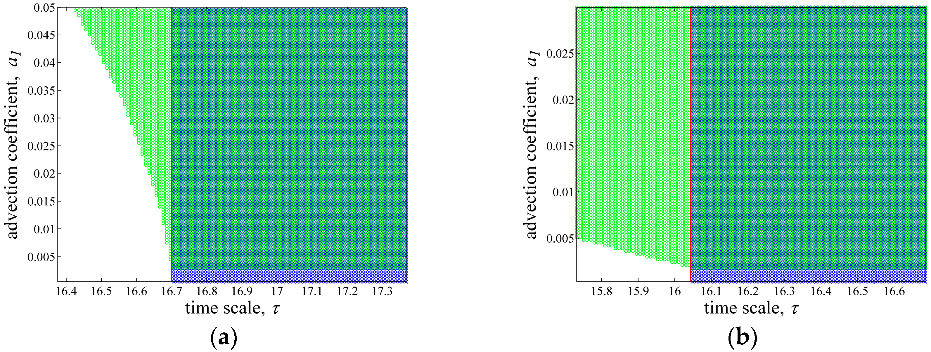
3.3. Parameter Space for Neimark-Sacker and Turing Bifurcation

Based on the bifurcation analysis above, parameters satisfying both Turing and Neimark-Sacker bifurcations will be selected to investigate the coupled effects of both bifurcations. Before that, we select two parameters which are parameter τ and a1, to show the parameter space for both bifurcations. τ is defined as the time step, it can reflect the frequency of wind events. However, as wind frequency is varying naturally (here we consider the real wind frequency, rather than the measured or recorded data), therefore, the variation of τ is meaningful and the four spatial parameters, D1, D2, a1 and a2, can reflect the values of wind speed, non-prevailing wind and prevailing wind, respectively. The previous study [26] gave that a1/a2 = D1/D2, and we mainly investigate prevailing wind. We can see that the variation of parameter a1 (parameter a2 will vary accordingly) represents the variation of prevailing wind speed. Note that wind, especially prevailing wind is the most important driving force in the process of vegetation pattern self-organization. Wind speed and frequency are the two key indexes of wind. Therefore, simulations on vegetation pattern self-organization will also be carried out through the variation of parameter τ and a1.
Figure 3 shows the parameter space that satisfies Turing and Neimark-Sacker bifurcations around bifurcation point τ0. Blue area and green area mean parameter values satisfy only Neimark-Sacker bifurcation and only Turing bifurcation respectively. In Figure 3a, τ0 = 16.6997 days. And in Figure 3b, τ0 = 16.0428 days. Given τ ∈ [0.98τ0, 1.04τ0] in both Figure 3a,b, we can see that Turing bifurcation area in Figure 3b is bigger than that in Figure 3a. And this will cause differences in the self-organization of patterns (will be shown in the next section). Turing-Neimark-Sacker bifurcation is defined as when parameter values satisfy both Turing and Neimark-Sacker bifurcations. Note that, we define the dark green area in Figure 3 as Turing-Neimark-Sacker bifurcation area. The condition for this area is:
τ > τ 0 , λ m ( 1 , 1 , τ ) > 1 , λ m m ( τ ) > λ m ( 1 , 1 , τ ) ,

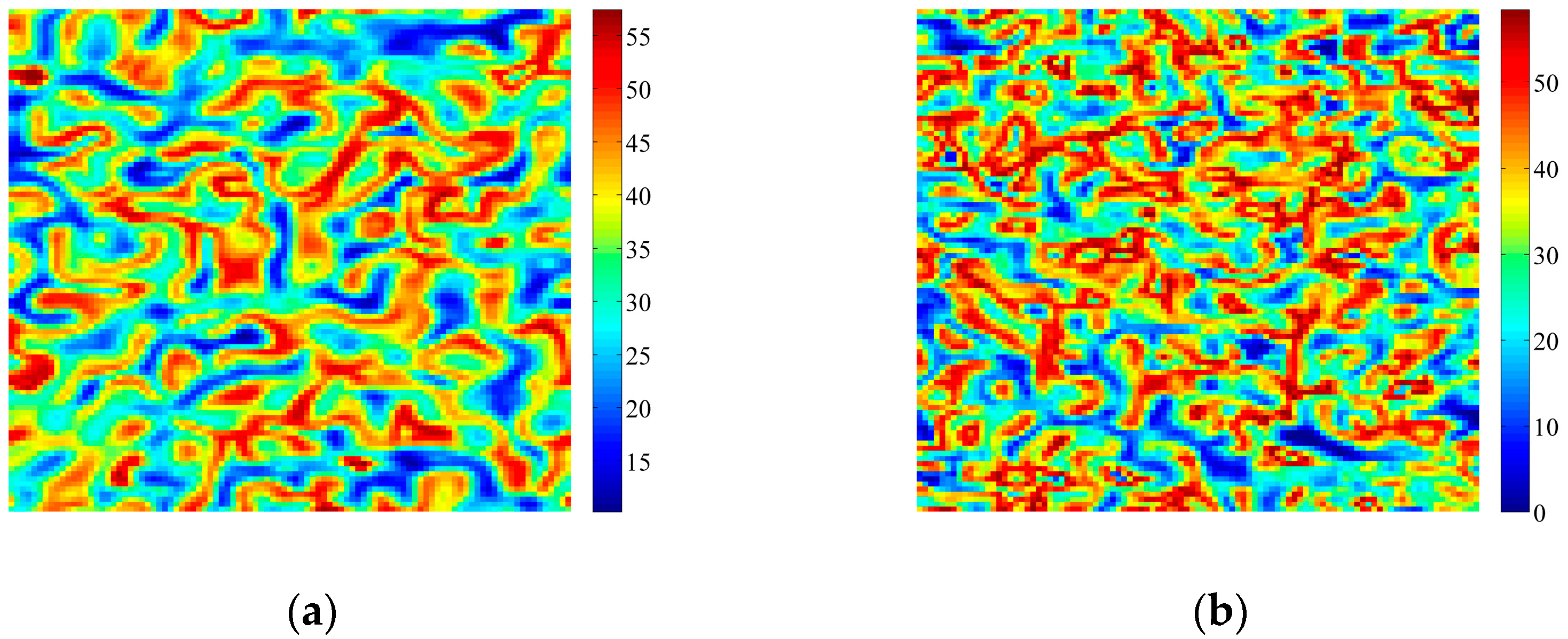
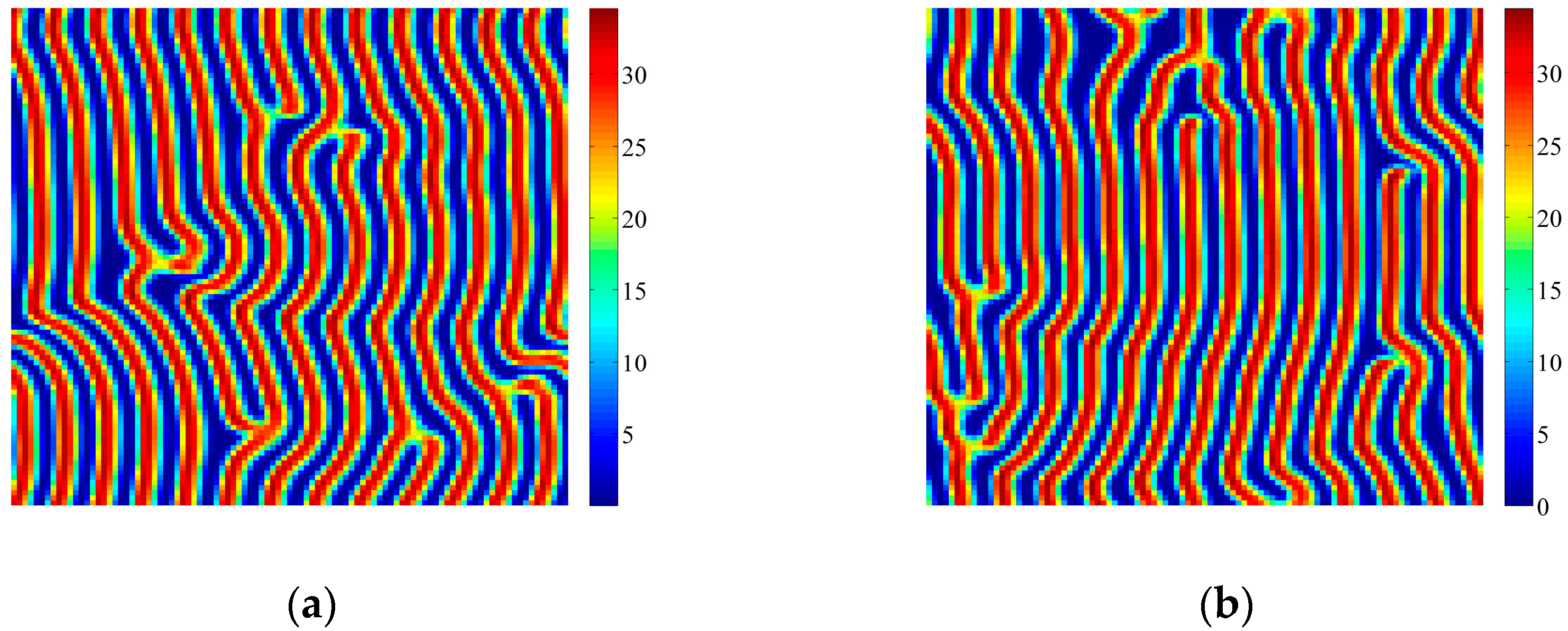
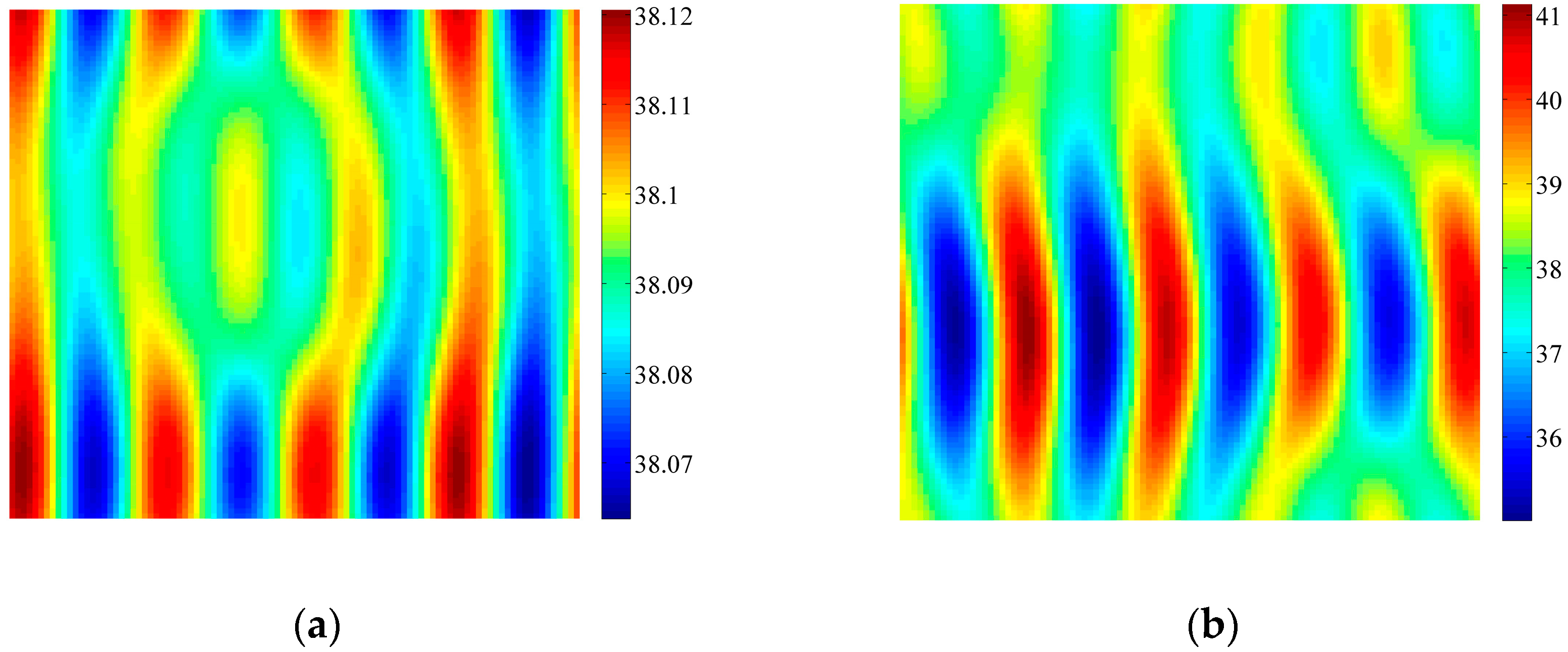
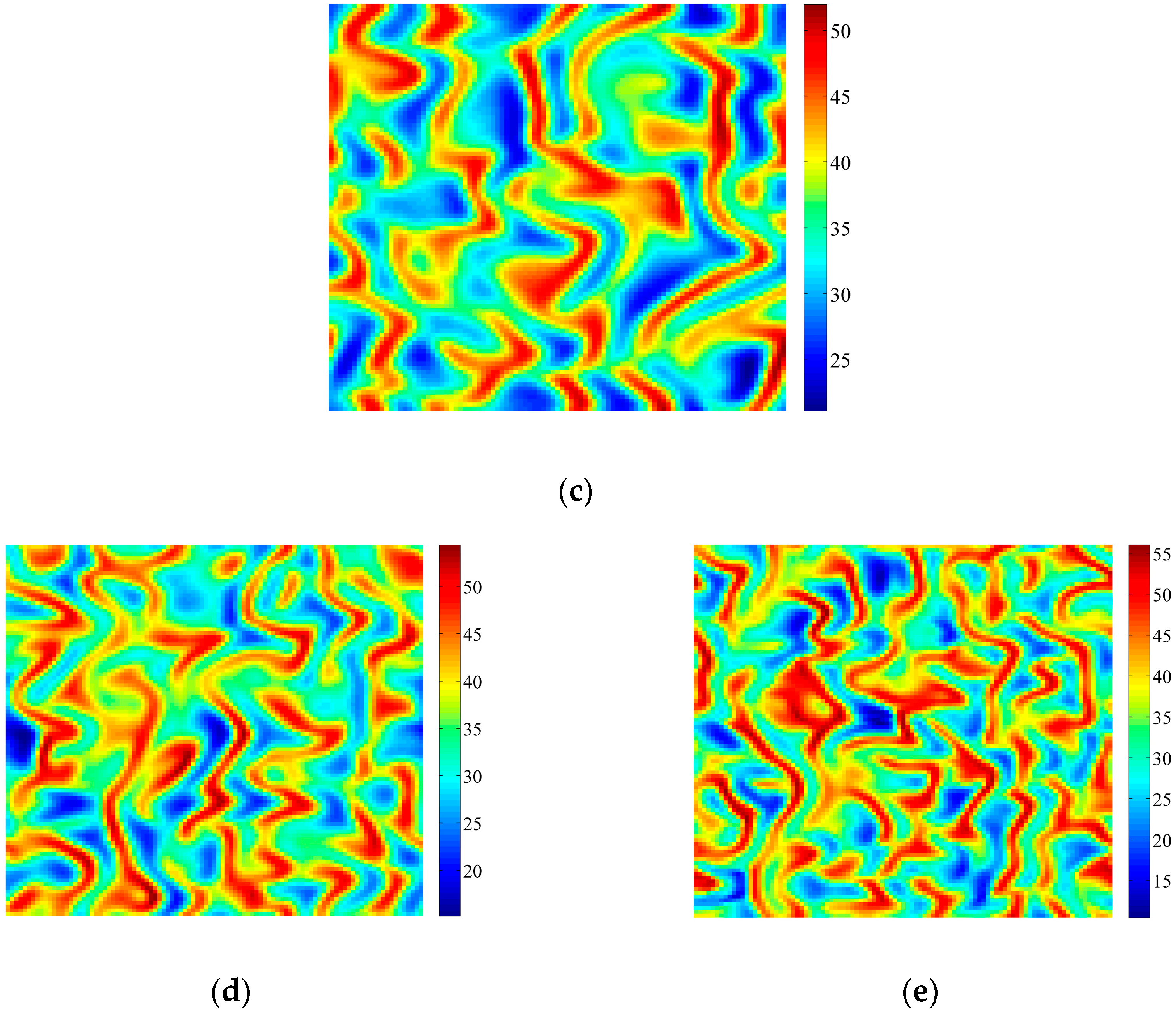
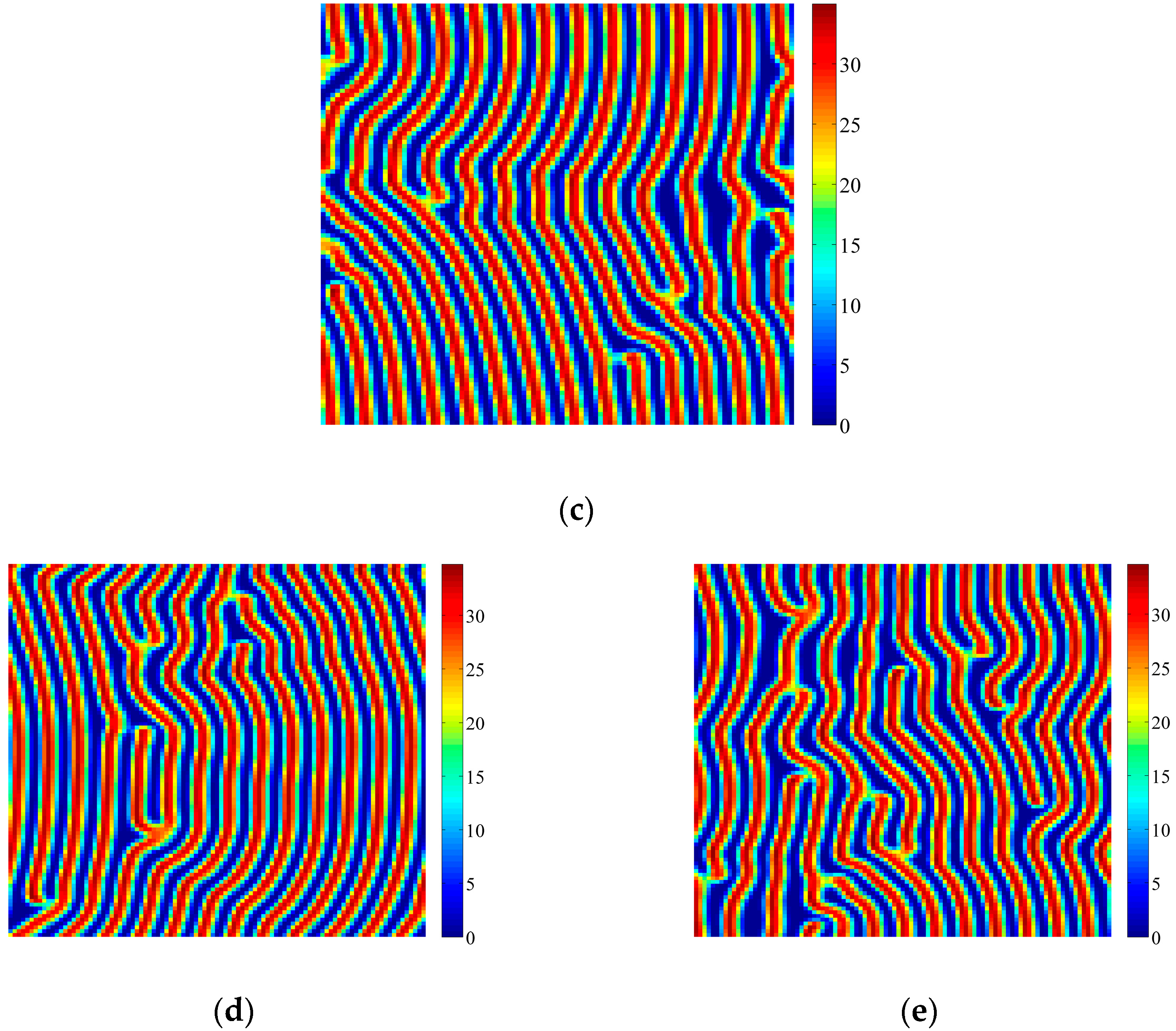
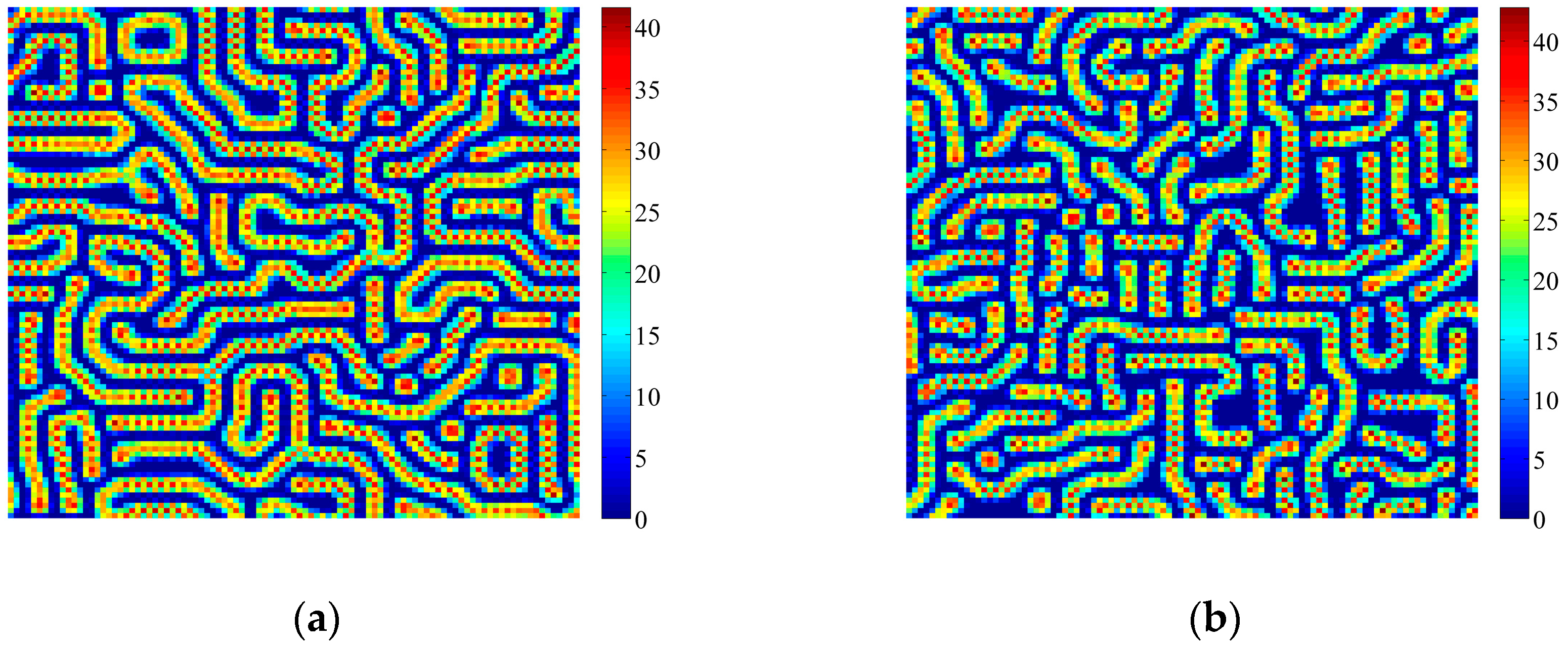
4. Coupled Effects of Turing and Neimark-Sacker Bifurcations on Vegetation Pattern Self-Organization

On the basis of the bifurcation analysis and the calculation of the parameter space for both Turing and Neimark-Sacker bifurcations, we will investigate the coupled effects of Turing and Neimark-Sacker bifurcation on vegetation pattern self-organization. Numerical simulations will be carried out around the bifurcation point τ0. With the increase of time scale τ, system will go through only Turing bifurcation to Turing-Neimark-Sacker bifurcation. Note that the color scale in all the following figures are automatically selected by the software MATLAB 7.12.0 (2011a) command “pcolor” according to the minimum and the maximum values of vegetation cover at each time. Precisely, the blue area represents low vegetation coverage, while the red area represents high vegetation coverage. Sometime, the minimum value of vegetation coverage reaches zero, which means vegetation dies out in the vegetation-sand system and only bare sand can be seen. Besides, after the simulation of vegetation pattern self-organization in each figure, the values of vegetation coverage will be mapped to the integers in the domain [1, 256] (which represents the 256 colors in the color spectrum), and then the Shannon entropy of each figure will be calculated.
Firstly, vegetation patterns induced by only Neimark-Sacker bifurcation are shown in Figure 4. Given parameters k0 = 3.095 cm·d−1, h = 0.2 d−1, Vm = 100%, p = 0.045 cm−1·d−1, m = 0.2 cm·d−1, n = 0.07 d−1, V0 = 200%, C = 10%, D1 = 0.01 m2·d−1, D2 = 0.01 m2·d−1, a1 = 0.01 m·d−1, a2 = 0.01 m·d−1, d = 2 m, Neimark-Sacker bifurcation occurs when τ = τ0 = 16.6997 days. When τ > 16.6997 days, spatially heterogenous vegetation patterns can be induced by the Neimark-Sacker bifurcation. With the increase of τ, wavelength of vegetation patterns becomes smaller, and the whole pattern becomes more complex as shown in Figure 4b. The type of the spatially heterogeneous vegetation patterns is complex and irregular, and difficult to define. In this research, we define it as the Neimark-Sacker type patterns. The values of entropy in Figure 4a,b are calculated as 7.7066 and 7.7708, respectively.
Figure 5 shows the transformation of vegetation patterns from under Turing bifurcation to under Turing-Neimark-Sacker bifurcation. Simulations are carried out around the Neimark-Sacker bifurcation point τ0 = 16.6997 days. When τ < τ0, Turing bifurcation occurs and Figure 5a,b show that regular striped vegetation patterns can be formed. Note that the amplitude of vegetation patterns in Figure 5a,b is not very big. When τ > τ0, Neimark-Sacker bifurcation and Turing bifurcation both occur, and vegetation patterns are changed. As shown in Figure 5c–e, we can see that pattern wavelength becomes smaller, stripes become narrower, curvy and irregular. Compared with the patterns in Figure 4, the vegetation patterns in Figure 5c–e are like stripes coupled with the Neimark-Sacker type patterns, but they are more similar to Neimark-Sacker type patterns. The values of entropy in Figure 5a–e are calculated as 5.8924, 7.8776, 7.5626, 7.5309 and 7.4856, respectively.
Figure 6 shows another series of vegetation patterns with the increase of time scale τ. When τ < τ0 = 16.0428 days, Turing bifurcation occurs and Figure 6a,b show that regular striped vegetation patterns with large amplitude can be formed. When τ > τ0, Neimark-Sacker bifurcation occurs. However the striped vegetation patterns seem unchanged as shown in Figure 6c–e. Obviously, these patterns are Turing type. The values of entropy in Figure 6a–e are calculated as 7.3101, 7.5809, 7.0303, 7.5018 and 7.3576, respectively. From Figure 5 and Figure 6, we can see that the coupled effects of Turing-Neimark-Sacker bifurcations can be different.
Figure 7 and Figure 8 will show two special situations of Turing-Neimark-Sacker bifurcations. From previous study, we know that without prevailing wind, labyrinth patterns can be obtained, while with prevailing wind, striped patterns can be formed. These two patterns will be shown in Figure 7 and Figure 8, respectively, and the effects of Turing-Neimark-Sacker bifurcations will be simulated.
Figure 7a,b show that labyrinth patterns can be induced by Turing bifurcation, but Neimark-Sacker bifurcations destroy the self-organizations and induces spots as shown in Figure 7c–e. With the increase of parameter τ, vegetation spots become less and more isolated. The values of entropy in Figure 7a–e are calculated as 7.1693, 6.9560, 3.5169, 2.1530 and 2.0576, respectively.
Figure 8a,b show that regular striped vegetation patterns can be induced by Turing bifurcation and Turing-Neimark-Sacker bifurcations induce the breakdown of the self-organizations as shown in Figure 8c–e. Vegetation stripes can also be formed, but the number and the width of vegetation stripes drastically decreases. With the increase of parameter τ, vegetation stripes become less and shorter. The values of entropy in Figure 8a–e are calculated as 7.0886, 6.3024, 2.3306, 4.1024 and 2.9138, respectively.
The different simulation results in Figure 5, Figure 6, Figure 7 and Figure 8 need to be discussed. From the comparison between Figure 5a and Figure 6a, we can see that the intensity of Turing bifurcation is different. Although we cannot assess the density of Turing bifurcation quantitatively, we can tell the relative intensity from the amplitude of the patterns. Clearly, the amplitude of vegetation patterns in Figure 6a is bigger than that in Figure 5a. Therefore, when Neimark-Sacker bifurcation also occurs, the coupled effects of Turing and Neimark-Sacker bifurcations will make Figure 5a more like Neimark-Sacker type patterns, and make Figure 6a more like Turing type patterns. Simulations in Figure 7 and Figure 8 show quite different results. From Figure 7 and Figure 8, we can see that vegetation patterns induced by Turing-Neimark-Sacker bifurcations are neither Turing type (especially Figure 7) nor Neimark-Sacker Type patterns. It seems that the coupled effects of Turing and Neimark-Sacker bifurcations make the degradation process of vegetation fiercer. Therefore, labyrinth patterns are broken down into spots, vegetation stripes become less. It is necessary to point out that simulations in Figure 7 and Figure 8 may depend on the special coupling of Turing and Neimark-Sacker bifurcations.
In the real world, vegetation bands are not perfectly straight. There have been several explanations on this issue. Some researchers think that this may be due to the stochastic micro-topography. There is another interpretation in [26], that the self-organization process takes a very long time (about 30,000 days). Before the regular bands are formed, the values of some parameters may change. For example, advection coefficients a1 and a2, as the speed and the direction of prevailing wind are changing all the time. Therefore, the patterns in the real world are curvy bands. In this research, we propose another possible explanation. We choose the parameter τ to be the varying parameter because the variation of time scale reflects the variation of wind frequency well. As wind frequency is changing all the time, the variation of τ becomes meaningful. Then the variation of τ causes the occurring of Neimark-Sacker bifurcation. Neimark-Sacker bifurcation and Turing bifurcation may occur at the same time. The coupled effects of Neimark-Sacker and Turing bifurcations make vegetation patterns more irregular and similar to real vegetation patterns in nature. Therefore, the irregular patterns of vegetation may be induced by the coupled effects of Neimark-Sacker and Turing bifurcation.
From the calculated values of entropy in all figures, we can see that the values of entropy don’t vary much in Figure 4, Figure 5 and Figure 6, but the values of entropy in Figure 7 and Figure 8 decrease drastically when Turing and Neimark-Sacker bifurcations both occur. The decrease of entropy reflects the decrease of information in the figures. This is consistent with what we can observe directly from the figures, as most vegetation dies out due to the coupled effects of Turing and Neimark-Sacker bifurcations, leaving only little vegetation.

5. Conclusions

The continuous model of wind-induced vegetation patterns is quite new and attractive. In this research, we transform it to a discrete model. The discretization of the continuous vegetation-sand model is due to the consideration that wind events and sand movements are both discrete. Based on the discrete model, this research considered Neimark-Sacker bifurcation, which was not considered in the previous study [26]. Special and complex vegetation patterns can be self-organized (Figure 4) when parameter values satisfy Neimark-Sacker bifurcation. Simulation results also show that labyrinth (as shown in Figure 7a,b) and striped vegetation patterns (as shown in Figure 6 and Figure 8a,b) can be obtained, which are the key results in [26]. Besides, with the increase of time scale τ, we simulated how vegetation patterns transform from Turing bifurcation to Turing-Neimark-Sacker bifurcation (Figure 5, Figure 6, Figure 7 and Figure 8). Especially the transformations from Figure 5a–e, the transformations from Figure 7a–e and the transformations from Figure 8a–e reveal the coupling effects of Turing and Neimark-Sacker bifurcations.
From all the bifurcation analysis, simulations and discussion, we can conclude that:
(a)
The method of discretization provides a new scenario in the study on wind-induced vegetation patterns. It preserves the patterns that can be obtained in [26].
(b)
After discretization, the variation of time scale becomes possible. This variation helps to understand pattern self-organization under different ecological scales.
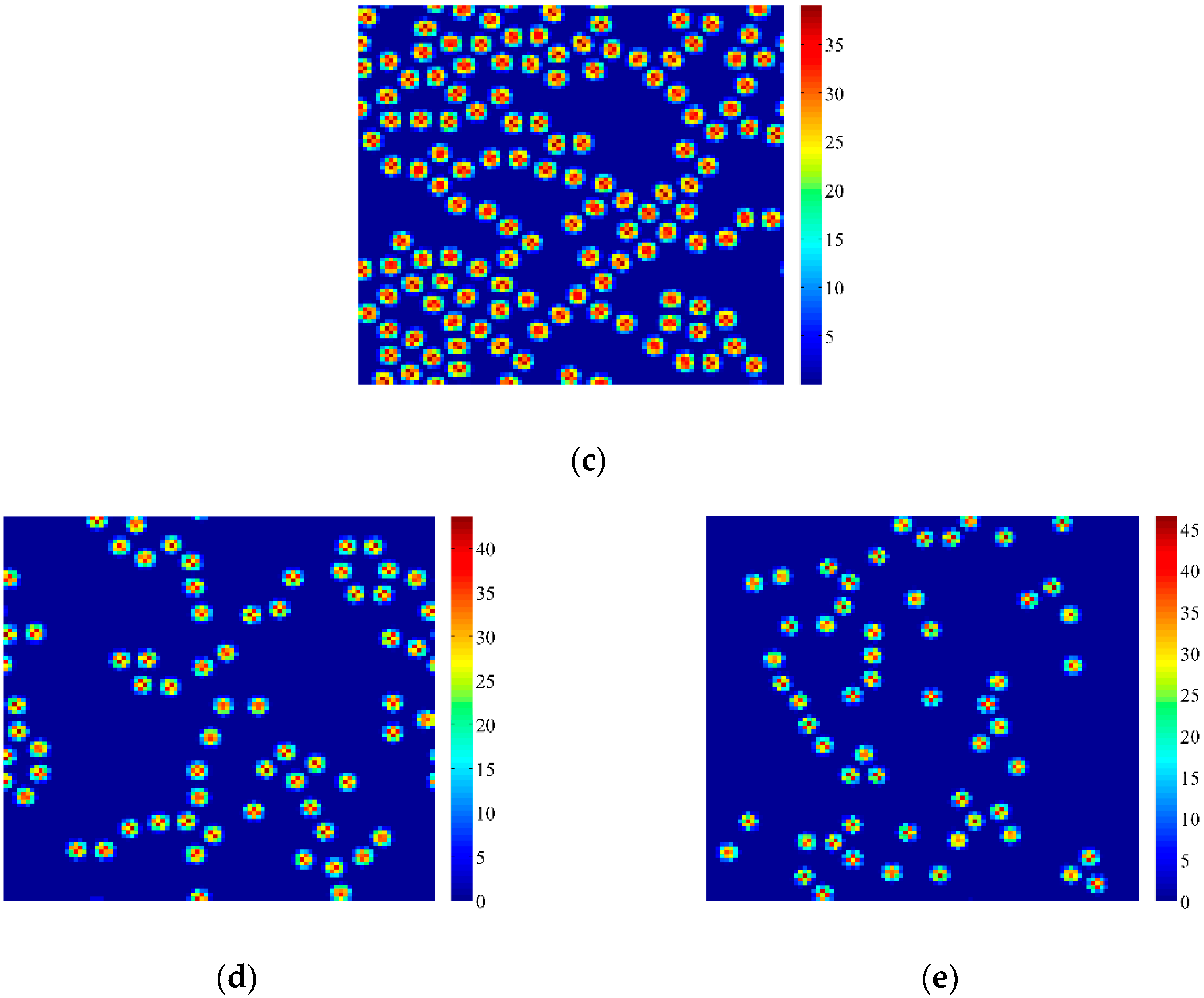
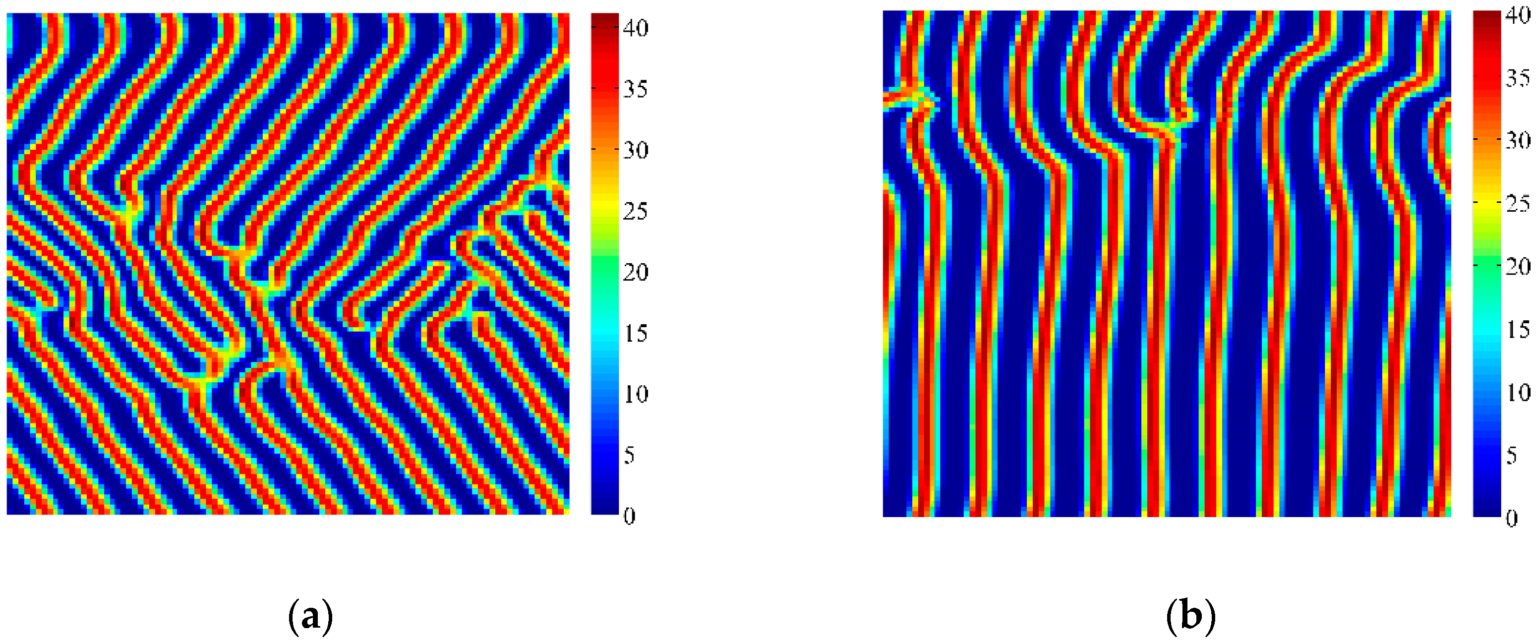
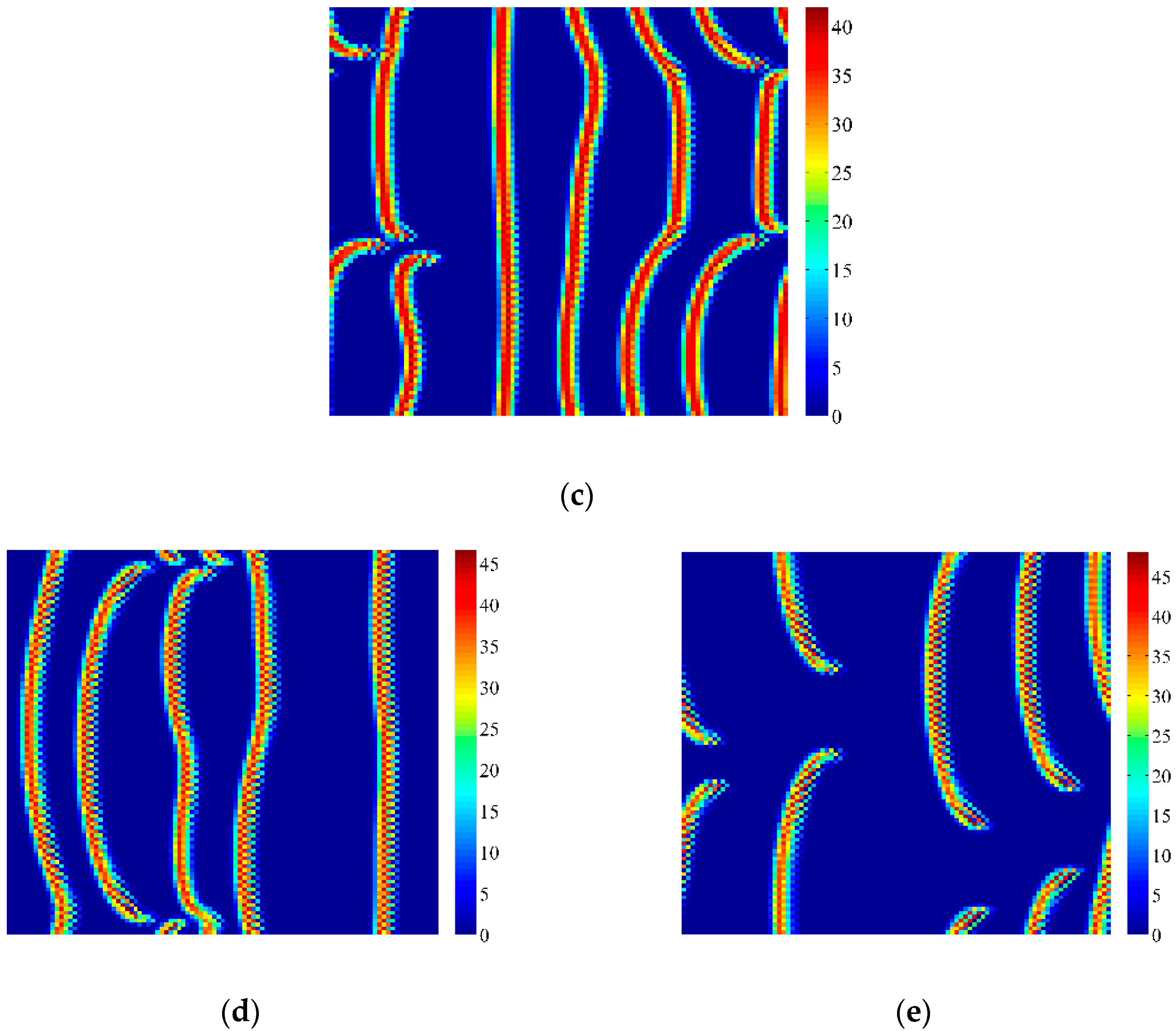
(c)
With the discrete vegetation-sand model, we investigated the coupled effects of Turing and Neimark-Sacker bifurcations. Under both bifurcation conditions, the type of simulated patterns depends on the intensity of each bifurcation. Sometime one bifurcation effect dominates the self-organization of patterns, while specially they couple with each other and lead to pattern variation, which can also be supported by the variance of entropy in Figure 7 and Figure 8. However, the coupled effects of Turing and Neimark-Sacker bifurcations are so complex that new methods may be needed to assess the intensity of each bifurcation.

Acknowledgments

The authors would like to acknowledge with great gratitude for the supports of Chinese Natural Science Foundation (Project 39560023 to H.Z.), National Special Water Programs (No. 2009ZX07210-009, No. 2015ZX07203-011, No. 2015ZX07204-007), the Fundamental Research Funds for the Central Universities (No. JB2017069), Department of Environmental Protection of Shandong Province (SDHBPJ-ZB-08). National Special Water Programs (No. 2017ZX07101).

Author Contributions

Tianxiang Meng and Shengnan Ma calculated the fixed points and stability analysis and verified the bifurcation conditions. Feifan Zhang did all the bifurcation conditions, simulations and wrote the paper. Huayong Zhang and Tousheng Huang gave some advice in the discussion, and Tousheng Huang performed modifications on the paper. All authors have read and approved the final manuscript.

Conflicts of Interest

The authors declare no conflict of interest.

Appendix A

Appendix A.1. Neimark-Sacker Bifurcation Analysis

First we transform the discrete model into a map, and we can obtain:
( S V ) ( S + τ ( k 0 + m V ( 1 V V 0 ) n S ) V + τ ( h V ( 1 V V m ) p S V C + V ) )
According to [41], Neimark-Sacker bifurcation requires three conditions. The first condition of Neimark-Sacker bifurcation requires the eigenvalues at fixed point λ1, λ2 are conjugate and their modules are 1, shown as:
λ 2 = λ 1 ¯ ,   | λ 1 | = | λ 2 | = 1 .
Then we get:
t r 0 2 4 Δ 0 < 0 ,   Δ 0 = 1 .
Which is:
( h n 2 h V 1 V m p S 1 C ( C + V 1 ) 2 ) 2 4 ( n h + 2 n h V 1 V m + n p S 1 C ( C + V 1 ) 2 + m p V 1 ( 2 V 1 + V 0 ) ( C + V 1 ) V 0 ) < 0
Then we can obtain the Neimark-Sacker bifurcation point τ0:
τ = τ 0 = n h + 2 h V 1 V m + p S 1 C ( C + V 1 ) 2 n h + 2 n h V 1 V m + n p S 1 C ( C + V 1 ) 2 + m p V 1 ( 2 V 1 + V 0 ) ( C + V 1 ) V 0
Let:
w = S S 1 , z = V V 1 ,
and we obtain a new map:
( w z τ ˜ ) ( a 11 w + a 12 z + a 13 2 z 2 + O ( ( | w | + | z | + | τ ˜ | ) 4 ) a 21 w + a 22 z + a 23 2 z 2 + a 24 w z + a 27 6 z 3 + a 28 2 w z 2     + O ( ( | w | + | z | + | τ ˜ | ) 4 ) τ ˜ )
In which:
a 11 = 1 n τ ,   a 12 = τ m ( 2 V 1 + V 0 ) V 0 , a 13 = 2 m τ V 0 ,   a 21 = τ p V 1 C + V 1 ,   a 22 = 1 + τ ( h 2 h V 1 V m p S 1 C ( C + V 1 ) 2 ) , a 23 = ( 2 C p S 1 ( C + V 1 ) 3 2 h V 1 m ) τ   ,   a 24 = τ p V 1 ( C + V 1 ) 2 τ p C + V 1 , a 27 = 6 C p S 1 τ ( C + V 1 ) 4 ,   a 28 = 2 τ p V 1 ( C + V 1 ) 3 + 2 τ p ( C + V 1 ) 2 ,
with τ = τ0.
The second condition of Neimark-Sacker bifurcation requires that:
d = d | λ ( τ ) | d τ | τ = τ 0 = 1 2 ( n h + 2 h V 1 V m + p S 1 C ( C + V 1 ) 2 ) 0
( λ ( τ 0 ) ) θ 1 ,   θ = 1 , 2 , 3 , 4
in which:
λ ( τ 0 ) ,   λ ¯ ( τ 0 ) = t r 0 ( τ 0 ) 2 ± i 2 4 Δ 0 ( τ 0 ) t r 0 2 ( τ 0 ) = α ± i β , i = 1 .
In which tr0(τ0) and ∆0(τ0) are described by Equation (12) with τ = τ0. Equation (A10) is equivalent to t r 0 ( τ 0 ) 2 , 1 , 0 , 2 . However, Equation (A3) requires that t r 0 ( τ 0 ) 2 , 2 , so from Equation (A10), we can obtain:
τ 0 ( n h + 2 h V 1 V m + p S 1 C ( C + V 1 ) 2 ) 2 , 3 .
The Neimark-Sacker bifurcation analysis will be performed based on the normal form of map (A7). Applying the invertible transformation:
( w z ) = ( a 12 0 α a 11 β ) ( w ˜ z ˜ ) ,
to map (A7), then the map becomes:
( w ˜ z ˜ ) ( α β β α ) ( w ˜ z ˜ ) + 1 a 12 β ( G 1 ( w ˜ , z ˜ ) G 2 ( w ˜ , z ˜ ) ) .
where:
G 1 ( w ˜ , z ˜ ) = a 13 2 β ( α a 11 ) 2 w ˜ 2 + a 13 2 β 3 z ˜ 2 a 13 β 2 ( α a 11 ) w ˜ z ˜ + O ( ( | w ˜ | + | z ˜ | ) 4 ) ,
G 2 ( w ˜ , z ˜ ) = ( ( a 13 2 ( α a 11 ) a 13 a 23 2 ) ( α a 11 ) 2 a 12 2 a 24 ( α a 11 ) ) w ˜ 2 + ( a 13 2 ( α a 11 ) a 13 a 23 2 ) β 2 z ˜ 2 + β ( a 12 2 a 24 ( a 13 ( α a 11 ) a 13 a 23 ) ( α a 11 ) ) w ˜ z ˜ ( a 12 2 a 28 2 + a 12 a 27 6 ( α a 11 ) ) ( α a 11 ) 2 w ˜ 3 a 12 β 2 ( a 12 a 28 2 + a 27 2 ( α a 11 ) ) w ˜ z ˜ 2 + a 12 ( α a 11 ) β ( a 12 a 28 + a 27 2 ( α a 11 ) ) w ˜ 2 z ˜ + a 12 a 27 6 β 3 z ˜ 3 + O ( ( | w ˜ | + | z ˜ | ) 4 ) .
The second-order and third-order partial derivatives of G 1 ( w ˜ , z ˜ ) and G 2 ( w ˜ , z ˜ ) at w ˜ = 0 and τ ˜ = 0 are calculated as:
G 1 w ˜ w ˜ = a 13 2 β ( α a 11 ) 2 , G 1 w ˜ z ˜ = a 13 β 2 ( α a 11 ) , G 1 z ˜ z ˜ = a 13 2 β 3 , G 1 w ˜ w ˜ w ˜ = G 1 w ˜ w ˜ z ˜ = G 1 w ˜ z ˜ z ˜ = G 1 z ˜ z ˜ z ˜ = 0 , G 2 w ˜ w ˜ = ( a 13 2 ( α a 11 ) a 13 a 23 2 ) ( α a 11 ) 2 a 12 2 a 24 ( α a 11 ) , G 2 w ˜ z ˜ = β ( a 12 2 a 24 ( a 13 ( α a 11 ) a 13 a 23 ) ( α a 11 ) ) , G 2 z ˜ z ˜ = ( a 13 2 ( α a 11 ) a 13 a 23 2 ) β 2 , G 2 w ˜ w ˜ w ˜ = ( a 12 2 a 28 2 + a 12 a 27 6 ( α a 11 ) ) ( α a 11 ) 2 , G 2 w ˜ w ˜ z ˜ = a 12 ( α a 11 ) β ( a 12 a 28 + a 27 2 ( α a 11 ) ) , G 2 w ˜ z ˜ z ˜ = a 12 β 2 ( a 12 a 28 2 + a 27 2 ( α a 11 ) ) , G 2 z ˜ z ˜ z ˜ = a 12 a 27 6 β
The third condition of Neimark-Sacker bifurcation requires:
a = Re ( ( 1 2 λ ¯ ) λ ¯ 2 1 λ ξ 11 ξ 20 ) 1 2 | ξ 11 | 2 | ξ 02 | 2 + Re ( λ ¯ ξ 21 ) 0 ,
in which:
ξ 20 = 1 8 ( ( F x ˜ x ˜ F y ˜ y ˜ + 2 G x ˜ y ˜ ) + i ( G x ˜ x ˜ G y ˜ y ˜ 2 F x ˜ y ˜ ) ) ,
ξ 11 = 1 4 ( ( F x ˜ x ˜ + F y ˜ y ˜ ) + i ( G x ˜ x ˜ + G y ˜ y ˜ ) ) ,
ξ 02 = 1 8 ( ( F x ˜ x ˜ F y ˜ y ˜ 2 G x ˜ y ˜ ) + i ( G x ˜ x ˜ G y ˜ y ˜ + 2 F x ˜ y ˜ ) ) ,
ξ 21 = 1 16 ( ( F x ˜ x ˜ x ˜ + F x ˜ y ˜ y ˜ + G x ˜ x ˜ y ˜ + G y ˜ y ˜ y ˜ ) + i ( G x ˜ x ˜ x ˜ + G x ˜ y ˜ y ˜ F x ˜ x ˜ y ˜ F y ˜ y ˜ y ˜ ) ) .
Then we can calculate a as:
a = A N M B 32 a 12 2 β 2 ( ( 1 α ) 2 + β 2 ) 1 32 a 12 2 β 2 ( ( G 1 w ˜ w ˜ + G 1 z ˜ z ˜ ) 2 + ( G 2 w ˜ w ˜ + G 2 z ˜ z ˜ ) 2 ) 1 64 a 12 2 β 2 ( ( G 1 w ˜ w ˜ G 1 z ˜ z ˜ 2 G 2 w ˜ z ˜ ) 2 + ( G 2 w ˜ w ˜ G 2 z ˜ z ˜ + 2 G 1 w ˜ z ˜ ) 2 ) + 1 16 a 12 β ( α ( G 2 w ˜ w ˜ z ˜ + G 2 z ˜ z ˜ z ˜ ) + β ( G 2 w ˜ w ˜ w ˜ + G 2 w ˜ z ˜ z ˜ ) ) 0
in which:
M = β ( 3 4 α ) ( α 2 β 2 ) 2 α β ( ( 1 α ) ( 1 2 α ) 2 β 2 ) , N = ( 1 3 α + 2 α 2 2 β 2 ) ( α 2 β 2 ) + ( 6 α 8 α 2 ) β 2 , A = ( G 1 w ˜ w ˜ + G 1 z ˜ z ˜ ) ( G 1 w ˜ w ˜ G 1 z ˜ z ˜ + 2 G 2 w ˜ z ˜ ) ( G 2 w ˜ w ˜ + G 2 z ˜ z ˜ ) ( G 2 w ˜ w ˜ G 2 z ˜ z ˜ 2 G 1 w ˜ z ˜ ) , B = ( G 2 w ˜ w ˜ + G 2 z ˜ z ˜ ) ( G 1 w ˜ w ˜ G 1 z ˜ z ˜ + 2 G 2 w ˜ z ˜ ) + ( G 1 w ˜ w ˜ + G 1 z ˜ z ˜ ) ( G 2 w ˜ w ˜ G 2 z ˜ z ˜ 2 G 1 w ˜ z ˜ ) .
When the conditions (A4), (A5), (A9), (A12) and (A23) are satisfied, Neimark-Sacker bifurcation occurs at (S1,V1). Besides, when a < 0 and d > 0, an attracting invariant circle bifurcates from (S1,V1) for τ > τ0; and when a > 0 and d > 0, a repelling invariant circle bifurcates for τ < τ0.

Appendix A.2. Turing Bifurcation Analysis

As we transformed the continuous model into a discrete one, the Turing bifurcation needs to be re-investigated. According to [42], Turing bifurcation requires two conditions. First, a nontrivial homogeneous stationary state exists and is stable to spatially homogeneous perturbations, which has been obtained in Section 2. Second, the stable stationary state is unstable to at least one type of spatially heterogeneous perturbations. Eigenvalues of discrete d and d 2 are different as those in continuous model, according to the method in [43], the eigenvalues of d can be obtained as:
λ k l 1 = 2 sin ϕ k exp ( ( ϕ k π 2 ) i ) .
where ϕ k = ( k 1 ) π / N , k { 1 , 2 , 3 , , N } and i represents the complex unit, that is i = 1 . While the eigenvalues of d 2 can be obtained as:
λ k l = 4 ( sin 2 ϕ k + sin 2 ϕ l ) ,
in which ϕ k = ( k 1 ) π / N , ϕ l = ( l 1 ) π / N , and k ,   l { 1 , 2 , 3 , , N } .
Spatially heterogeneous perturbations are introduced to perturb the stable homogeneous stationary state (S1,V1). The spatially heterogeneous perturbations on S and V are given by:
S ˜ ( i , j , t ) = S ( i , j , t ) S 1 ,
V ˜ ( i , j , t ) = V ( i , j , t ) V 1 .
Noticing d 2 S ˜ ( i , j , t ) = d 2 S ( i , j , t ) and d 2 V ˜ ( i , j , t ) = d 2 V ( i , j , t ) . Substituting Equations (A27) and (A28) into Equations (2)–(5) leads to:
S ˜ ( i , j , t + 1 ) = a 11 ( S ˜ ( i , j , t ) + τ d a 1 d S ˜ ( i , j , t ) + τ d 2 D 1 d 2 S ˜ ( i , j , t ) ) + a 12 ( V ˜ ( i , j , t ) + τ d a 2 d V ˜ ( i , j , t ) + τ d 2 D 2 d 2 V ˜ ( i , j , t ) ) + O ( ( | S ˜ ( i , j , t ) | + | V ˜ ( i , j , t ) | ) 2 ) ,
V ˜ ( i , j , t + 1 ) = a 21 ( S ˜ ( i , j , t ) + τ d a 1 d S ˜ ( i , j , t ) + τ d 2 D 1 d 2 S ˜ ( i , j , t ) ) + a 22 ( V ˜ ( i , j , t ) + τ d a 2 d V ˜ ( i , j , t ) + τ d 2 D 2 d 2 V ˜ ( i , j , t ) ) + O ( ( | S ˜ ( i , j , t ) | + | V ˜ ( i , j , t ) | ) 2 ) ,
where a11, a12, a21 and a22 are described by Equation (A8). The two-order terms in Equations (A29) and (A30) can be ignored when the perturbations are small. Through simple calculation, we can obtain:
d ( d 2 ( X i j ) ) = d 2 ( d ( X i j ) ) ,
Therefore, we can use the corresponding eigenfunction X k l i j of the eigenvalue λkl to multiply Equations (A29) and (A30), and obtain:
X k l i j S ˜ ( i , j , t + 1 ) = a 11 X k l i j S ˜ ( i , j , t ) + a 12 X k l i j V ˜ ( i , j , t ) + τ d a 11 X k l i j d S ˜ ( i , j , t ) + τ d a 12 X k l i j d V ˜ ( i , j , t ) + τ d 2 a 11 X k l i j d 2 S ˜ ( i , j , t ) + τ d 2 a 12 δ X k l i j d 2 V ˜ ( i , j , t ) ,
X k l i j V ˜ ( i , j , t + 1 ) = a 21 X k l i j S ˜ ( i , j , t ) + a 22 X k l i j V ˜ ( i , j , t ) + τ d a 21 X k l i j d S ˜ ( i , j , t ) + τ d a 22 X k l i j d V ˜ ( i , j , t ) + τ d 2 a 21 X k l i j d 2 S ˜ ( i , j , t ) + τ d 2 a 22 δ X k l i j d 2 V ˜ ( i , j , t ) .
Summing Equations (A32) and (A33) for all i and j obtains:
X k l i j S ˜ ( i , j , t + 1 ) = a 11 X k l i j S ˜ ( i , j , t ) + a 12 X k l i j V ˜ ( i , j , t ) + τ d 2 a 11 X k l i j d 2 S ˜ ( i , j , t ) + τ d 2 a 12 δ X k l i j d 2 V ˜ ( i , j , t ) ,
X k l i j V ˜ ( i , j , t + 1 ) = a 21 X k l i j S ˜ ( i , j , t ) + a 22 X k l i j V ˜ ( i , j , t ) + τ d 2 a 21 X k l i j d 2 S ˜ ( i , j , t ) + τ d 2 a 22 δ X k l i j d 2 V ˜ ( i , j , t ) .
Let S ¯ t = X k l i j S ˜ ( i , j , t + 1 ) and V ¯ t = X k l i j V ˜ ( i , j , t + 1 ) , Equations (A34) and (A35) can be transformed into the following form:
S ¯ t + 1 = a 11 ( 1 + τ d a 1 λ k l 1 τ d 2 D 1 λ k l ) S ¯ t + a 12 ( 1 + τ d a 2 λ k l 1 τ d 2 D 2 λ k l ) V ¯ t ,
V ¯ t + 1 = a 21 ( 1 + τ d a 1 λ k l 1 τ d 2 D 1 λ k l ) S ¯ t + a 22 ( 1 + τ d a 2 λ k l 1 τ d 2 D 2 λ k l ) V ¯ t .
Equations (A36) and (A37) describes the dynamics of spatially heterogeneous perturbations integrating all the lattices. If Equations (A36) and (A37) converge, the discrete system will go back to the spatially homogeneous stationary state. Only the divergence of Equations (A36) and (A37) can lead to the breaking of homogeneous state and the self-organization of Turing patterns. Calculating the two eigenvalues associated with Jacobian matrix of Equations (A36) and (A37) obtains:
λ ± ( k , l , τ ) = 1 2 t r ( k , l , τ ) ± 1 2 t r ( k , l , τ ) 2 4 Δ ( k , l , τ ) ,
in which:
t r ( k , l , τ ) = t r 0 ( τ ) + τ d ( a 11 ( τ ) a 1 + a 22 ( τ ) a 2 ) a 1 λ k l 1 + τ d 2 ( a 11 ( τ ) D 1 + a 22 ( τ ) D 2 ) λ k l ,
Δ ( k , l , τ ) = Δ 0 ( τ ) ( 1 + τ d a 1 λ k l 1 D 1 τ d 2 λ k l ) ( 1 + τ d a 2 λ k l 1 τ d 2 D 2 δ λ k l ) .
Here tro(τ), ∆0(τ), a11(τ), and a22(τ) are denoted for reminding that they are dependent on τ. Based on the two eigenvalues, define:
λ m ( k , l , τ ) = max ( | λ + ( k , l ) | ,   | λ ( k , l ) | ) ,
λ m m ( τ ) = max k = 1 , l = 1 N λ m ( k , l , τ ) .
where λmm(τ) represents the maximal value of absolute modulus of both eigenvalues in Equation (A41). When λmm(τ) > 1, Turing instability occurs; when λmm(τ) < 1, the discrete system stabilizes at the homogeneous states. Therefore, the threshold condition for the occurrence of Turing bifurcation requires λmm(τ) = 1.

References

  1. Klausmeier, C.A. Regular and irregular patterns in semiarid vegetation. Science 1999, 284, 1826–1828. [Google Scholar] [CrossRef] [PubMed]
  2. Deblauwe, V.; Couteron, P.; Bogaert, J.; Barbier, N. Determinants and dynamics of banded vegetation pattern migration in arid climates. Ecol. Monogr. 2012, 82, 3–21. [Google Scholar] [CrossRef]
  3. Muller, J. Floristic and structural pattern and current distribution of tiger bush vegetation in Burkina Faso (West Africa), assessed by means of belt transects and spatial analysis. Appl. Ecol. Environ. Res. 2013, 11, 153–171. [Google Scholar] [CrossRef]
  4. Berg, S.S.; Dunkerley, D.L. Patterned mulga near Alice Springs, central Australia, and the potential threat of firewood collection on this vegetation community. J. Arid Environ. 2004, 59, 313–350. [Google Scholar] [CrossRef]
  5. Moreno, M.L.H.; Saco, P.M.; Willgoose, G.R.; Tongway, D.J. Variations in hydrological connectivity of Australian semiarid landscapes indicate abrupt changes in rainfall-use efficiency of vegetation. J. Geophys. Res. 2012, 117, G03009. [Google Scholar] [CrossRef]
  6. Montan, C. The colonization of bare areas in two-phase mosaics of an arid ecosystem. J. Ecol. 1992, 80, 315–327. [Google Scholar] [CrossRef]
  7. McDonald, A.K.; Kinucan, R.J.; Loomis, L.E. Ecohydrological interactions within banded vegetation in the northeastern Chihuahuan Desert, USA. Ecohydrology 2009, 2, 66–71. [Google Scholar] [CrossRef]
  8. HilleRisLambers, R.; Rietkerk, M.; van den Bosch, F.; Prins, H.; de Kroon, H. Vegetation pattern formation in semi-arid grazing systems. Ecology 2001, 82, 50–61. [Google Scholar] [CrossRef]
  9. Rietkerk, M.; Boerlijst, M.C.; van Langevelde, F.; HilleRisLambers, R.; van de Koppel, J.; Kumar, L.; Prins, H.H.T.; de Roos, A.M. Self-organization of vegetation in arid ecosystems. Am. Nat. 2002, 160, 524–530. [Google Scholar] [PubMed]
  10. Lefever, R.; Lejeune, O. On the origin of tiger bush. Bull. Math. Biol. 1997, 59, 263–294. [Google Scholar] [CrossRef]
  11. D’Odorico, P.; Laio, F.; Ridolfi, L. Vegetation patterns induced by random climate fluctuations. Geophys. Res. Lett. 2006, 33, L19404. [Google Scholar] [CrossRef]
  12. D’Odorico, P.; Laio, F.; Porporato, A.; Ridolfi, L.; Barbier, N. Noise-induced vegetation patterns in fire-prone savannas. J. Geophys. Res. 2007, 112, G02021. [Google Scholar] [CrossRef]
  13. Sherratt, J.A. An analysis of vegetation stripe formation in semi-arid landscapes. J. Math. Biol. 2005, 51, 183–197. [Google Scholar] [CrossRef] [PubMed]
  14. Van de Koppel, J.; Rietkerk, M.; Van, L.F.; Kumar, L.; Klausmeier, C.A.; Fryxell, J.M.; Hearne, J.W.; van Andel, J.; de Ridder, N. Spatial heterogeneity and irreversible vegetation change in semiarid grazing systems. Am. Nat. 2002, 159, 209–218. [Google Scholar] [CrossRef] [PubMed]
  15. D’Odorico, P.; Laio, F.; Ridolfi, L. Patterns as indicators of productivity enhancement by facilitation and competition in dryland vegetation. J. Geophys. Res. 2006, 111, G03010. [Google Scholar] [CrossRef]
  16. Haken, H. Information and Self-Organization; Springer: Berlin, Germany, 1988. [Google Scholar]
  17. Nicolis, J.S. Chaos and Information Processing; World Scientific: Singapore, 1999. [Google Scholar]
  18. Mahara, H.; Yamaguchi, T. Calculation of the Entropy Balance Equation in a Non-equilibrium Reaction-diffusion System. Entropy 2010, 12, 2436–2449. [Google Scholar] [CrossRef]
  19. Nicolis, G.; Nicolis, C. Stochastic Resonance, Self-Organization and Information Dynamics in Multistable Systems. Entropy 2016, 18, 172. [Google Scholar] [CrossRef]
  20. Mezghani, N.; Mitiche, A.; Cheriet, M. Maximum Entropy Gibbs Density Modeling for Pattern Classification. Entropy 2012, 14, 2478–2491. [Google Scholar] [CrossRef] [Green Version]
  21. Clayton, W.D. Vegetation ripples near Gummi, Nigeria. J. Ecol. 1966, 54, 415–417. [Google Scholar] [CrossRef]
  22. Clayton, W.D. The vegetation of Katsina province, Nigeria. J. Ecol. 1969, 57, 445–451. [Google Scholar] [CrossRef]
  23. Zonneveld, I. A geomorphological based banded “tiger” pattern related to former dune fields in Ž. Sokoto, northern Nigeria. Catena 1999, 37, 45–56. [Google Scholar] [CrossRef]
  24. White, L.P. Vegetation arcs in Jordan. J. Ecol. 1969, 57, 461–464. [Google Scholar] [CrossRef]
  25. White, L.P. Vegetation stripes on sheet wash surfaces. J. Ecol. 1971, 59, 615–622. [Google Scholar] [CrossRef]
  26. Zhang, F.; Zhang, H.; Evans, M.R.; Huang, T. Vegetation patterns generated by a wind driven sand-vegetation system in arid and semi-arid areas. Ecol. Complex. 2017, 31, 21–33. [Google Scholar] [CrossRef]
  27. Okin, G.S.; Murray, B.; Schlesinger, W.H. Degradation of sandy arid shrubland environments: Observations, process modelling, and management implications. J. Arid Environ. 2001, 47, 123–144. [Google Scholar] [CrossRef]
  28. Eldridge, D.J.; Leys, J.F. Exploring some relationships between biological soil crusts, soil aggregation and wind erosion. J. Arid Environ. 2003, 53, 457–466. [Google Scholar] [CrossRef]
  29. Yan, Y.C.; Xu, X.L.; Xin, X.P.; Yang, G.X.; Wang, X.; Yan, R.R.; Chen, B.R. Effect of vegetation cover on aeolian dust accumulation in a semiarid steppe of northern China. Catena 2011, 87, 351–356. [Google Scholar] [CrossRef]
  30. Zhao, H.L.; Zhou, R.L.; Drake, S. Effects of aeolian deposition on soil properties and crop growth in sandy soils of northern China. Geoderma 2007, 142, 342–348. [Google Scholar] [CrossRef]
  31. Zhang, F.F.; Zhang, H.Y.; Huang, T.S. Dynamics on the interaction between vegetation growth and aeolian dust deposition. Adv. Mater. Res. 2012, 356–360, 2430–2433. [Google Scholar] [CrossRef]
  32. Wang, W.; Lin, Y.; Zhang, L.; Rao, F.; Tan, Y. Complex patterns in a predator–prey model with self and cross-diffusion. Commun. Nonlinear Sci. 2011, 16, 2006–2015. [Google Scholar] [CrossRef]
  33. Mistro, D.C.; Rodrigues, L.A.D.; Petrovskii, S. Spatiotemporal complexity of biological invasion in a space-and time-discrete predator-prey system with the strong Allee effect. Ecol. Complex. 2012, 9, 16–32. [Google Scholar] [CrossRef]
  34. Han, Y.T.; Han, B.; Zhang, L.; Xu, L.; Li, M.F.; Zhang, G. Turing instability and wave patterns for a symmetric discrete competitive Lotka-Volterra system. WSEAS Trans. Math. 2011, 10, 181–189. [Google Scholar]
  35. Punithan, D.; Kim, D.K.; McKay, R.I.B. Spatio-temporal dynamics and quantification of daisy world in two-dimensional coupled map lattices. Ecol. Complex. 2012, 12, 43–57. [Google Scholar] [CrossRef]
  36. Rodrigues, L.A.D.; Mistro, D.C.; Petrovskii, S. Pattern formation in a space- and time-discrete predator-prey system with a strong Allee effect. Theor. Ecol. 2012, 5, 341–362. [Google Scholar] [CrossRef]
  37. Huang, T.; Zhang, H.; Yang, H.; Wang, N.; Zhang, F. Complex patterns in a space- and time-discrete predator-prey model with Beddington-DeAngelis functional response. Commun. Nonlinear Sci. Numer. Simul. 2017, 43, 182–199. [Google Scholar] [CrossRef]
  38. Yuan, S.; Xu, C.; Zhang, T. Spatial dynamics in a predator-prey model with herd behavior. Chaos Interdiscip. J. Nonlinear Sci. 2013, 23, 033102. [Google Scholar] [CrossRef] [PubMed]
  39. Zhang, T.H.; Xing, Y.P.; Zang, H.; Han, M. Spatio-temporal dynamics of a reaction–diffusion system for a predator–prey model with hyperbolic mortality. Nonlinear Dyn. 2014, 78, 265–277. [Google Scholar] [CrossRef]
  40. Zhang, T.; Zang, H. Delay-induced Turing instability in reaction-diffusion equations. Phys. Rev. E 2014, 90, 052908. [Google Scholar] [CrossRef] [PubMed]
  41. Guckenheimer, J.; Holmes, P. Nonlinear Oscillations, Dynamical Systems and Bifurcations of Vector Fields; Springer: New York, NY, USA, 1983. [Google Scholar]
  42. Turing, A. The chemical basis of morphogenesis. Philos. Trans. R. Soc. Lond. B 1952, 237, 37–72. [Google Scholar] [CrossRef]
  43. Bai, L.; Zhang, G. Nontrivial solutions for a nonlinear discrete elliptic equation with periodic boundary conditions. Appl. Math. Comput. 2009, 210, 321–333. [Google Scholar] [CrossRef]
Figure 1. Bifurcation diagram and phase portraits of flip bifurcation. (a) Bifurcation diagram with parameters: k0 = 3.095 cm·d−1; h = 0.2 d−1; Vm = 100%; p = 0.045 cm−1·d−1; m = 0.2 cm·d−1; n = 0.07 d−1; V0 = 200%; C = 10%; D2 = 0.01 m2·d−1; (bd) Phase portraits with parameter (b) τ = 16.7013 days; (c) τ = 16.755 days; (d) τ = 16.8667 days. Note that the figures are obtained by the software MATLAB 7.12.0 2011a (The MathWorks, Inc., Natick, MA, USA).
Entropy 19 00478 g001aEntropy 19 00478 g001b
Figure 2. Variations of eigenvalues λm(k,l) with perturbation numbers k and l. Parameters: k0 = 3.095 cm·d−1; h = 0.2 d−1; Vm = 100%; p = 0.045 cm−1·d−1; m = 0.2 cm·d−1; n = 0.07 d−1; V0 = 200%; C = 10%; D1 = 0.01 m2·d−1; D2 = 0.01 m2·d−1; a2 = 0.01 m·d−1; (a) a1 = 0.15 m·d−1; (b) Let k = l, three curves of eigenvalues λm(k,l) are shown with parameter a1 = 0.005, 0.027 and 0.15 m·d−1 respectively. Note that the color scale in all the following figures are automatically selected by the MATLAB 7.12.0 (2011a) software command “pcolor” according to the minimum and the maximum values of λm(k,l).
Entropy 19 00478 g002
Figure 3. Variations of parameter τ and a1 satisfying Turing and Neimark-Sacker bifurcations around bifurcation point. Parameters: h = 0.2 d−1; Vm = 100%; p = 0.045 cm−1·d−1; m = 0.2 cm·d−1; n = 0.07 d−1; V0 = 200%; C = 10%; D1 = 0.01 m2·d−1; D2 = 0.01 m2·d−1; a2 = 0.01 m·d−1; (a) k0 = 3.095 cm·d−1; d = 2 m; (b) k0 = 3.83 cm·d−1; d = 1 m. Light green area means parameter values satisfy only Turing bifurcation condition. Blue area means parameter values satisfy only Neimark-Sacker bifurcation. And Dark green area means parameter values satisfy both Turing and Neimark-Sacker bifurcation. Note that the figures are obtained by the software MATLAB 7.12.0 (2011a).
Entropy 19 00478 g003
Figure 4. Patterns induced by Neimark-Sacker bifurcations. Parameters: k0 = 3.095 cm·d−1; h = 0.2 d−1; Vm = 100%; p = 0.045 cm−1·d−1; m = 0.2 cm·d−1; n = 0.07 d−1; V0 = 200%; C = 10%; D1 = 0.01 m2·d−1; D2 = 0.01 m2·d−1; a1 = 0.01 m·d−1; a2 = 0.01 m·d−1; d = 2 m; (a) τ = 18.3696 days; (b) τ = 20.0396 days. Simulations are carried out on 100 × 100 lattices with periodic boundary conditions. Initial conditions are set as fixed points with heterogeneous random disturbance (0.5%). After t = 2000 days, the patterns can be obtained.
Entropy 19 00478 g004
Figure 5. Patterns induced by Turing and Turing-Neimark-Sacker bifurcations. Parameters: k0 = 3.095 cm·d−1, h = 0.2 d−1, Vm = 100%, p = 0.045 cm−1·d−1, m = 0.2 cm·d−1, n = 0.07 d−1, V0 = 200%, C = 10%, D1 = 0.02 m2·d−1, D2 = 0.01 m2·d−1, a1 = 0.04 m·d−1, a2 = 0.02 m·d−1, d = 2 m. (a) τ = 16.2822 days; (b) τ = 16.3323 days; (c) τ = τ0 = 16.6997 days; (d) τ = 17.0337 days; (e) τ = 17.3677 days. Simulations are carried out on 100 × 100 lattices with periodic boundary conditions. Initial conditions are set as fixed points with heterogeneous random disturbance (0.5%). After t = 2000 days, the patterns can be obtained.
Entropy 19 00478 g005aEntropy 19 00478 g005b
Figure 6. Patterns induced by Turing and Turing-Neimark-Sacker bifurcations. Parameters: k0 = 3.83 cm·d−1, h = 0.2 d−1, Vm = 100%, p = 0.045 cm−1·d−1, m = 0.2 cm·d−1, n = 0.07 d−1, V0 = 200%, C = 10%, D1 = 0.014 m2·d−1, D2 = 0.01 m2·d−1, a1 = 0.0196 m·d−1, a2 = 0.014 m·d−1, d = 1 m. (a) τ = 15.4011 days; (b) τ = 15.7219 days; (c) τ = τ0 = 16.0428 days; (d) τ = 16.0909 days; (e) τ = 16.1230 days. Simulations are carried out on 100 × 100 lattices with periodic boundary conditions. Initial conditions are set as fixed points with heterogeneous random disturbance (0.5%). After t = 2000 days, the patterns can be obtained.
Entropy 19 00478 g006aEntropy 19 00478 g006b
Figure 7. Patterns induced by Turing and Turing-Neimark-Sacker bifurcations. Parameters: k0 = 3.865 cm·d−1, h = 0.2 d−1, Vm = 100%, p = 0.045 cm−1·d−1, m = 0.2 cm·d−1, n = 0.07 d−1, V0 = 200%, C = 10%, D1 = 0.015 m2·d−1, D2 = 0.01 m2·d−1, a1 = 0 m·d−1, a2 = 0 m·d−1, d = 1 m. (a) τ = 21.6614 days; (b) τ = 21.8825 days; (c) τ = τ0 = 22.1035 days; (d) τ = 22.3245 days; (e) τ = 22.5456 days. Simulations are carried out on 100 × 100 lattices with periodic boundary conditions. Initial conditions are set as fixed points with heterogeneous random disturbance (0.5%). After t = 2000 days, the patterns can be obtained.
Entropy 19 00478 g007aEntropy 19 00478 g007b
Figure 8. Patterns induced by Turing and Turing-Neimark-Sacker bifurcations. Parameters: k0 = 3.83 cm·d−1, h = 0.2 d−1, Vm = 100%, p = 0.045 cm−1·d−1, m = 0.2 cm·d−1, n = 0.07 d−1, V0 = 200%, C = 10%, D1 = 0.015 m2·d−1, D2 = 0.01 m2·d−1, a1 = 0.225 m·d−1, a2 = 0.015 m·d−1, d = 1 m. (a) τ = 15.4011 days; (b) τ = 15.7219 days; (c) τ = τ0 = 16.0428 days; (d) τ = 16.0909 days; (e) τ = 16.1230 days. Simulations are carried out on 100 × 100 lattices with periodic boundary conditions. Initial conditions are set as fixed points with heterogeneous random disturbance (0.5%). After t = 2000 days, the patterns can be obtained.
Entropy 19 00478 g008aEntropy 19 00478 g008b

