A Characterization of the Domain of Beta-Divergence and Its Connection to Bregman Variational Model

School of Liberal Arts, Korea University of Technology and Education, Cheonan 31253, Korea
Entropy 2017, 19(9), 482; https://doi.org/10.3390/e19090482
Submission received: 20 July 2017
/
Revised: 4 September 2017
/
Accepted: 7 September 2017
/
Published: 9 September 2017
(This article belongs to the Special Issue Entropy in Signal Analysis)
Abstract
:In image and signal processing, the beta-divergence is well known as a similarity measure between two positive objects. However, it is unclear whether or not the distance-like structure of beta-divergence is preserved, if we extend the domain of the beta-divergence to the negative region. In this article, we study the domain of the beta-divergence and its connection to the Bregman-divergence associated with the convex function of Legendre type. In fact, we show that the domain of beta-divergence (and the corresponding Bregman-divergence) include negative region under the mild condition on the beta value. Additionally, through the relation between the beta-divergence and the Bregman-divergence, we can reformulate various variational models appearing in image processing problems into a unified framework, namely the Bregman variational model. This model has a strong advantage compared to the beta-divergence-based model due to the dual structure of the Bregman-divergence. As an example, we demonstrate how we can build up a convex reformulated variational model with a negative domain for the classic nonconvex problem, which usually appears in synthetic aperture radar image processing problems.
1. Introduction
In general, the domain of a divergence [1,2] is that confined not by the positiveness of variables but by the positiveness of a divergence (i.e., ). Therefore, the domain of a divergence could be defined to include negative region while keeping positiveness of the divergence. To the best of our knowledge, it is unclear when the domain of the -divergence (and the corresponding Bregman-divergence) include the negative region. In this article, we systematically explore the domains of the -divergence [2] and the corresponding Bregman-divergence associated with the convex function of Legendre type [3].
The -divergence [2,4,5,6,7] is a general framework of similarity measures induced from various statistical models, such as Poisson, Gamma, Gaussian, Inverse Gaussian, compound Poisson, and Tweedie distribution. For the connection between the -divergence and the various statistical distributions, see [8]. Among the diverse statistical distributions, the Tweedie distribution has a unique feature, i.e., the unit deviance of the Tweedie distribution [8] corresponds to the -divergence with . It is interesting that is a vital range of while defining a convex right Bregman proximity operator [9,10]. We will address this issue in more details in Section 4. In addition, the -divergence is also used as a distance-like measure in diverse areas, for instance, synthetic aperture radar (SAR) image processing [11,12], audio spectrogram comparison [6,13], and brain EEG signal processing [7].
We note that authors in [7] show the usefulness of the -divergence with as a robust similarity measure against outliers between two probability distributions. Here, outliers (rare events) are that have extremely low probability and thus they exist near zero probability. However, the (generalized) Kullback–Leibler-divergence (i.e., -divergence ), which is a commonly used similarity measure for probability distributions, is undefined at zero (). See Figure 1a. Therefore, it is not easy to obtain robustness against outliers through the (generalized) Kullback–Leibler-divergence. On the contrary, the -divergence with (i.e., ) is well defined at zero () and thus it is more robust to outliers than the Kullback–Leibler-divergence. For more details, see [4,5,7]. We also note that if the variables of -divergence are not probability distributions (i.e., unnormalized) then outliers correspond to the variables that have extremely large values (≫1) [14]. To detect such kind of outliers under the Gamma distribution assumption, the -divergence with is used as a distance-like measure in [11]. See also Figure 1c.
In the case of SAR image data processing, speckle noise is modeled with the Gamma distribution and thus the negative log-likelihood function, which appears in speckle reduction problem, corresponds to the -divergence with , i.e., the Itakura–Saito-divergence. Actually, this model is highly nonconvex [15]. Therefore, various transforms are introduced to relax nonconvexity of the Gamma distribution related speckle reduction model [16,17,18,19,20,21]. Recently, we have shown that the -divergence with can be used as a transform-less convex relaxation model for SAR speckle reduction problem [12]. Generally, the data captured via a SAR system has extremely high dynamic range [22,23]. Under this harsh environment, -divergence with is successfully used as a similarity measure for separation of the strong scatterers in SAR data [11]. In addition, the -divergence is also used for the decomposition of magnitude data of audio spectrograms [6]. In these applications, the domains of data are generally assumed to be positive. However, the domain of the -divergence can be extended to the negative region. In fact, if , then the -divergence is exactly the square of -distance, the domain of which naturally includes a negative region. Surprisingly, in this article, we show that, under the mild condition on , there are infinitely many -divergences that have a negative domain.
It is known that the -divergence can be reformulated with the Bregman-divergence [2,6]. However, if we restrict the base function of the Bregman-divergence as the convex function of Legendre type, then some part of the -divergence cannot be expressed through the Bregman-divergence (see Table 1). Although the Bregman-divergence associated with a convex function of Legendre type does not exactly match with the -divergence, due to the fruitful mathematical structure of the convex function of Legendre type, the associated Bregman-divergence has many useful properties. For instance, the dual formulation of the Bregman-divergence associated with the convex function of Legendre type can be used as a convex reformulation of some nonconvex problems under the certain condition on its domain [24]. In this article, we demonstrate that, by using the dual Bregman-divergence with the negative convex domain, we can make a convex reformulated Bregman variational model for the classic nonconvex problem that appears in the SAR image noise reduction problem [15]. We also show that we can unify the various variational models appearing in image processing problems as the Bregman variational model having sparsity constraints, e.g., total variation [25,26] (we called it Bregman-TV). Actually, the Bregman variational model corresponds to the right Bregman proximity operator [9,10]. See also [9,10,24,27,28,29,30] for theoretical analysis of the Bregman-divergence and related interesting properties of it.
1.1. Background
In this section, we review typical examples of the -divergence, i.e., Itakura–Saito-divergence, Generalized Kullback–Leibler-divergence (I-divergence), and -distance. In addition, we introduce the Bregman-divergence and the corresponding Bregman variational model with sparsity constraints.
Let us start with the -divergence given by
where is the domain of the -divergence. Actually, the domain corresponds to the effective domain in optimization [3,31]. We call and as the left and right domains of the -divergence. In addition, we assume that the left and right domains, and , are convex sets, respectively. That is, if (or ), then the line segment between two points also satisfies (or ). Note that , , , is the all one vector in , , , , and . In addition, integration, multiplication, and division are performed component-wise. Based on a selection of , we can recover the famous representatives of the -divergence, i.e., Itakura–Saito-divergence [4,5,13], I-divergence (or generalized Kullback–Leibler-divergence) [20,32], and -distance [25,26]. These three divergences are important examples of the -divergence, since they show three different types of domains of the -divergence. We summarize them in the following.
- Itakura–Saito-divergence (): andUsually, the left and right domain, i.e., and of Itakura–Saito-divergence, are defined as positive and [12,13]. However, due to the scale invariance property of it, the variables b and u can be negative at the same time, even within the logarithmic function, i.e., . Based on this keen observation, in this article, we develop a new methodology that systematically detects a domain having the negative region. The Itakura–Saito-divergence is a typical example that can be expressed by the -divergence and the Bregman-divergence at the same time. However, it has the negative domain in the -divergence framework, but not in the Bregman-divergence framework (see Table 1).
- Generalized Kullback–Leibler-divergence (I-divergence) (): andwhere we naturally assume that Interestingly, it has different left and right domains, i.e., . Due to the asymmetric structure of the domain of I-divergence, we need to carefully handle the -divergence at the boundary of each domain. We categorize the class of the -divergence that has the asymmetric domain structure in Section 2.
- -distance (): andThis divergence is preferable to other divergences, since it has as its domain for each variable. Unlike the previous two divergences, the domain of it naturally includes a negative region . Surprisingly, there are infinitely many -divergences having as its domain. We will show it in Section 2.
Additionally, we introduce the Bregman-divergence associated with the convex function of Legendre type [3]. The Bregman-divergence is formulated as
where the base function is the convex function of Legendre type [3], , and is the interior of . In fact, it is relatively interior of , i.e., . Note that is the interior of relative to its affine hull, which is the smallest affine set including . Therefore, the relative interior coincides with the interior when the affine hull of is . For more details, see Chapter 2.H in [31]. In this article, since the -divergence (1) is separable in terms of dimension, the affine hull of is always and thus we simply use instead of . Note that the typical examples of the -divergence in the above (Itakura–Saito-divergence, I-divergence, and -distance) can be reformulated with the Bregman-divergence (2) by using the convex function of Legendre type and the associated domain :
- Itakura–Saito-divergence: with
- I-divergence: with
- -distance: with
The domain of the second variable of the Bregman-divergence (2) is always open set . However, the right domain of the second variable of the -divergence (1) could be a closed set. In the coming section, we thoroughly analyze the relation between the Bregman-divergence and the -divergence with regard to its domain. Based on the Bregman-divergence (2), we introduce the Bregman variational model that unifies the various minimization problems appearing in image processing:
where b is the observed data and is the sparsity enforcing regularization term, such as total variation [26]. In image processing, (3) corresponds to the denoising problem under the various noise distributions: Poisson, Speckle, Gaussian noise, etc. However, in optimization, it is known as (nonconvex) right Bregman proximity operator under mild conditions. See [9,10,24,30] for more details on the Bregman operator.
1.2. Overview
The article is organized as follows. In Section 2, we analyze the structure of the domain of the -divergence. In Section 3, we study various mathematical structures of the -divergence through the Bregman-divergence associated with the convex function of Legendre type. In Section 4, we introduce the Bregman variational model and its dual formulation for convex reformulation of the classic nonconvex problem that appears in the SAR speckle reduction problem. In addition, we introduce the right and left Bregman proximal operator. We give our conclusions in Section 5.
2. A Characterization of the Domain of the -Divergence
In this section, we analyze the structure of the -divergence and the associated domain based on the so-called extended logarithmic function.
Let us start with a definition of the extended logarithmic function that is essential in characterizing the domain of the -divergence. We note that it corresponds to an equivalence class of Tsallis’s generalized logarithmic function [1,33] with an extention to the negative domain.
Definition 1.
Let and
where and Then, the extended logarithmic function is defined as an equivalence class
For simplicity, we leave out all constants after integration and then we attain
where . We call (4) as the extended logarithmic function instead of the equivalence class , unless otherwise specified.
Note that the domain and range of (4) are given in Table 2. In addition, we illustrate the structure of the extended logarithmic function in Figure 2. As noticed in Definition 1, the extended logarithmic function is defined as an equivalence class with respect to c. If we set then we can recover Tsallis’ generalized logarithmic function [1,33] on its positive domain . See Figure 2a. However, we cannot use the generalized logarithm (i.e., ) in the negative domain. In fact, if and then Tsallis’ generalized logarithmic function is undefined, e.g., . On the other hand, the proposed extended logarithmic function (4) is well defined on for all , since we can choose an appropriate c having the same sign with u even if , e.g., . See Figure 2d and Table 2. Indeed, the extended logarithmic function is useful when we simplify the complicated structure of the -divergence. As described in the following Definition 2, the -divergence is defined based on the difference of two extended logarithmic functions. In other words, the -divergence is invariance with respect to a constant function in the extended logarithmic function (4). It is interesting that the Bregman-divergence (2) also has a similar invariance property with respect to an affine function in the base function (see Proposition 1).
Definition 2.
Let and . Then, the β-divergence is defined by
After integration, we get the well-known formula of β-divergence:
Although the -divergence has a unified formula (5) via the extended logarithm (4), unfortunately, the determination of the domain of the -divergence heavily depends on . Before we go any further, let us introduce the most important equivalence classes in this article. It will simplify complicated notations appearing in the -divergence and the Bregman-divergence.
Note that and are subsets of the rational number and satisfy , while is composed of all irrational numbers with a subset of the rational number that are not in . For instance, , and .
Since the -divergence (6) is developed based on the extended logarithmic function (i.e., power functions), inherently, we have to quantify the domain of a power function and its inverse function Actually, if x is positive, then a power function and the corresponding inverse function is well defined, irrespective of the choice of an exponent . On the other hand, in the case of negative domain, e.g., , the domain of a power function severely depends on the choice of an exponent . With newly introduced equivalence classes in (7), we can easily categorize the domain of a power function and its inverse function . We summarize it in the following Lemma.
Lemma 1.
Let and be the negative domain of a power function Then, has its negative domain
and the corresponding range
In addition, if then the inverse function of p is well defined and transparent on , i.e., for all . However, if then for all .
Proof.
For any , let then the power function p is expressed as We note that the negative real domain of is well-defined only if . To clarify the evaluation of , let us express it in a polar form:
Then, we get
where Regarding the inverse function we have for all However, if then That is, we have , for all ☐
Now, with the equivalence classes (7) and Lemma 1, we classify domains of the -divergence. The details are given in the following Theorem and Table 3. See also Figure 1 for the overall structure of the -divergence on its domain.
Theorem 1.
Let us consider the domain of the β-divergence
where
and In addition, let us assume that the minimum value of on its domain is nonnegative, i.e.,
where Then, the domain of the β-divergence is classified as in Table 3. Note that for all . In particular, if then
Proof.
Due to the assumption , we can easily obtain the positiveness of the -divergence by the following inequality
Consequently, we only need to fulfill the following two conditions: (1) Is the domain of the -divergence determined to satisfy (9)? (2) Is the -divergence well-defined on its domain?
- Case 1: for all .If then it is trivial to show and thus it is always true that . Now, we will find such that is satisfied. From Lemma 1, if then, we get the followingBased on , we have two different cases regarding the domain
- Case 2: for all .Basically, the -divergence can be expressed asThat is, it is based on integrations of power functions of real variables u and b in . Therefore, we only need to see whether or not the integration in is well defined at We note that, after integration, the exponents of and are different and thus the corresponding domains and could be different as well. Hence, we should consider the following three different cases:
- -
- : We do not have any singularity at with respect to and . Therefore, we have
- -
- : After integration, does not have any singularity at . However, has a singularity at . Therefore, we have but and thus in this region.
- -
- : In this case, both and have singularity at . Thus,
Based upon the analysis in Cases 1 and 2, we have six different choices of domain for the -divergence. It is summarized in Table 3 and illustrated in Figure 1. Since we only consider a convex domain, and should be selected as a convex set for each variable. In addition, due to the inherent integral formulation of -divergence between b and u, the domain of both variables should be determined to have the same sign. ☐
As observed in Table 3, if , then there is a symmetry in the selection of the domain of the -divergence. That is, or Especially, if , then the -divergence corresponds to the Itakura–Saito-divergence where the domain of it can be or The positive domain is generally preferable, since it is related to real applications, e.g., intensity data type in the SAR system [11,12]. However, if we reformulate the -divergence with the Bregman-divergence, then the negative domain commonly appears in the dual Bregman-divergence. In addition, we note that, due to Theorem 1, the -divergence with the domain defined in Table 3 satisfies the following distance-like properties of the generic divergence [1,2]:
where (11) is followed from the Definition of the domain of the -divergence and (10). Note that (12) is satisfied, if we restrict the domain of the -divergence as In fact, let us assume that . It is trivial to show that . Therefore, we only need to show . Letting , we then get from (10).
Since the -divergence (5) with its domain defined in Table 3 has the distance-like properties, (11) and (12), we can make a variational model with the -divergence and a regularization term for smoothness constraint of the given data b. The following is an example of a variational model based on the -divergence [12]
where and is a domain of for a given . Note that B is an open convex set induced from the physical constraints of the observed data b. In the case of a prior , it can be a sparsity-enforcing function such as total variation (TV) [25,26] and frame [34]. We call (13) the β-sparse model or β-TV [12], if TV is used as a prior. Under the domain restriction in Table 3, actually, we have lots of freedom in choosing of the -sparse model (13). However, if we add additional constraints, such as convexity onto the -divergence, then interestingly, the possible choice of is dramatically reduced to a small set. For example, with respect to u is convex on its domain only if [6]. Outside of this region, i.e., , the convexity of it depends on the given data b [12]. In Section 4.1, we analyze the convexity of the -divergence via the right Bregman proximity operator [28].
Although the proposed -sparse model in (13) is not convex in general, has an interesting global optimum property [11,12], in case . See also [35,36]. For completeness of the article, we add it below.
Theorem 2 ([11,36]).
For a given observed data , let B be an open convex set in , and Then, we obtain that
is always satisfied, regardless of the choice of
Note that in (14) corresponds to the -centroid in segmentation problem and is related to the Bregman centroid, which is extensively studied in [37]. In SAR image processing, if , then (14) corresponds to the multi-looking process, which is commonly used to reduce speckle noise in SAR data [12,22,23].
3. The Bregman-Divergence Associated with the Convex Function of Legendre Type for the -Divergence
In this section, we study the Bregman-divergence associated with the convex function of Legendre type and its connection to the -divergence. Although there is partial equivalence between two divergences, the Bregman-divergence has an important mathematical dual formulation. With a negative domain, the dual Bregman-divergence is unambiguously useful for convex reformulation of the nonconvex -sparse model (13) (see Section 4).
Before we proceed further, let us first review the convex function of Legendre type (see Section 26 [3]). See also [27,29].
Definition 3.
Let be lower semicontinuous, convex, and proper function defined on . Then, Φ is the convex function of Legendre type (or Legendre), if the following conditions are satisfied (i.e., Φ is essentially strictly convex and essentially smooth):
- 1.
- 2.
- Φ is differentiable on
- 3.
- and
- 4.
- Φ is strictly convex on
Here, is a convex set and is the boundary of the domain Ω.
The main advantage of the convex function of Legendre type is that the inverse function of the gradient of it has an isomorphism with the gradient of its conjugate function as described below. This is a useful property when we characterize the dual structure of the Bregman-divergence associated with the convex function of Legendre type.
Theorem 3 ([3,27]).
Let and Then, the function Φ is the convex function of Legendre type if and only if its conjugate
is the convex function of Legendre type. In this case, the gradient mapping
is an isomorphism with its inverse mapping .
For more details on Theorem 3, see Theorem 26.5 in [3] and Fact 2.9 in [27]. Let us assume that be the convex function of Legendre type. Then, we can define the Bregman-divergence associated with Legendre :
where and . Several functions we are interested in are in a category of the convex function of Legendre type. For instance, Shannon entropy function is a typical example of Legendre. the Bregman-divergence associated with it corresponds to the -divergence with i.e., Generalized Kullback–Leibler-divergence. We note that there is the convex function of Legendre type which does not have a corresponding -divergence. For instance, Fermi–Dirac entropy function is Legendre and the associated Bregman divergence is the Logistic loss function See [27,36] for more details on the Bregman-divergence. In the following, we summarize various useful features of the Bregman-divergence associated with Legendre .
Theorem 4.
Let and Then, the Bregman-divergence associated with the convex function of Legendre type Φ satisfies the following.
- 1.
- is strictly convex with respect to b on .
- 2.
- For any , is coercive with respect to b, i.e.,
- 3.
- For some , is coercive with respect to u if and only if .
- 4.
- if and only if where
- 5.
- For anywhere is the conjugate function of Φ.
- 6.
- For any
Proof.
Since is the convex function of Legendre type, is strictly convex on . Hence, is trivial. The proofs of – are in Theorem 3.7, Theorem 3.9 and Corollary 3.11 in [27]. ☐
In the above Theorem, the dual formulation (17) is a unique feature of the Bregman-divergence with Legendre. Unfortunately, the -divergence does not have a corresponding dual concept. Later, we will show how to use the dual Bregman-divergence (17) to make a convex reformulated model of the nonconvex -sparse model (13). In addition, we note that the -divergence (5) is established based on the extended logarithmic function (4), which is an equivalence class in terms of a constant function. Therefore, we can say that the -divergence is invariant with respect to a constant function in the extended logarithmic function. Interestingly, the base function of the Bregman-divergence also has such kind of invariance property with respect to an affine function. For this, does not need to be Legendre. However, for simplicity, we assume that is Legendre. The details are following.
Proposition 1.
Let us define an equivalence class of the convex function of Legendre type Φ in terms of affine function as follows:
where Then, the Bregman-divergence associated with an equivalence class is equal to the Bregman-divergence associated with Φ, irrespective of the choice of an affine function .
Proof.
We have the following equivalence with respect to an arbitrary affine function :
where and Therefore, with an arbitrary affine function (i.e., an equivalence class in terms of affine function ) does not change the structure of the Bregman-divergence at all. ☐
To connect the -divergence and the Bregman-divergence associated with Legendre, we need to find a specialized convex function of Legendre type. Based on the comments in [2], we use an integral formula of the extended logarithmic function for the special convex function of Legendre type. Through this connection, we can reformulate the -divergence into the Bregman-divergence associated with the convex function of Legendre type. The details are following.
Theorem 5.
Proof.
For simplicity, all affine functions are left out based on Proposition 1. In addition, it is trivial to show that is the Burg entropy ( with ) if and the Shannon entropy ( with ) if . They are well-known examples of Legendre. As noticed in (2), the corresponding Bregman-divergences are Itakura–Saito-divergence and Generalized Kullback–Leibler-divergence.
Now, we only need to check whether () is Legendre or not. Among four conditions in Definition 3, it is trivial to show that satisfies the conditions 1 and 2. In the end, with and two Legendre conditions 3 and 4 are left.
- I.
- Condition 3 in Definition 3:Since () is a power function, the only possible boundary of is . Therefore, we search to find where condition 3 is satisfied. Since , we get the following at the potential boundary
- -
- :
- -
- :
In summary, the following are the possible domains and the corresponding for condition 3. We note that, if , then :- -
- and
- -
- and
- II.
- Condition 4 in Definition 3:It can be easily checked by the fact that is strictly convex on if and only if is strictly monotone, that is, the following is satisfied [38] :Since is separable in terms of dimension, we only need to show that is a strictly increasing function on Note that if on an open region, then is strictly convex (i.e., is strictly increasing) in that region:
- -
- if and
- -
- if and
Note that at , we need to directly show that is strictly increasing.
Now, we integrate the information in the above Legendre conditions 3 and 4 for the decision of the domain based on . The details are the following:
- -
- and Therefore, is strictly increasing function on since
- -
- but is an odd function with respect to zero and thus it is not a convex function.
- -
- but it does not satisfy condition 3 at .
- -
- but is not a convex set. Since [3], to keep convexity of the domain we need to select or That is, we have or In both cases, we know that is strictly increasing on , since .
- -
- Following the case , we have or If , then is strictly increasing on (). However, if , then and thus it is not convex on its negative domain.
- -
- and is strictly increasing function on since for all
- -
- Condition 3 is satisfied on the above selected domain.
- -
- is not a convex set. Therefore, we need to restrict as a convex set, i.e., or . On both domains, is strictly increasing ().
- -
- Following the case we have or If then is strictly increasing on
- -
- and is strictly increasing function on since for all
- -
- Condition 3 is satisfied on the above selected domain.
☐
Remark 1.
Since in (19) is Legendre under the domain condition (20), we can establish a new Bregman-divergence associated with in (19). Interestingly, it corresponds to the -divergence (1) [2]. However, there is a mismatch between the domain of the Bregman-divergence in (20) and the domain of the -divergence in Table 3. We summarize it in Table 1. As a matter of fact, the positive domain with is not defined in (19) due to the Legendre condition. In addition, in the case of , the negative domain is not defined in the Bregman-divergence with (19). In the following Theorem, we show that under the restriction of the domain of the -divergence to the domain of the Bregman-divergence, we can get an equivalence between the -divergence and the Bregman-divergence associated with Legendre (19).
Theorem 6.
Let us consider the β-divergence (1) and the Bregman-divergence (16) associated with Legendre Φ (19). If we restrict the domain of the β-divergence with the domain of the Bregman-divergence associated with Φ (19), which is (see Table 1), then the β-divergence is equal to the Bregman-divergence associated with Legendre Φ(19).
Proof.
Since the domain of the -divergence is set up with , the -divergence is well defined with the restricted domain. In the following, we show an equivalence between the -divergence and the Bregman-divergence under the domain condition of the Bregman-divergence:
Note that we do not use any information in the above derivation and thus the above equivalence is well satisfied within the domain of the Bregman-divergence associated with Legendre (19). ☐
In the following Theorem, we calculate the conjugate function and the corresponding domain of the convex function of Legendre type defined in (19). The computation of the domain of is useful in determining the structure of . For instance, as noticed in Theorem 4 (3), if is open, then the corresponding Bregman-divergence is coercive with respect to . Surprisingly, when , is not convex but coercive with respect to u. This fact is importantly used in SAR speckle reduction problems [12,15,21].
Theorem 7.
Let Φ (19) be the convex function of Legendre type with (20). Then, , the conjugate of Φ, and the corresponding domain is calculated as follows:
- and :
- and :
- In this case, depends on β:
Proof.
Since is Legendre, from Theorem 3, if then we have
As noticed in (20), the domain of (19) depends on and thus the domain of its conjugate function also depends on . We categorize below, by using (22):
- and From (22), the conjugate function is calculated asTherefore, the domain of becomes
- and From (22), the conjugate function is calculated asIt is trivial to show that
- and is given in (20). By simple calculation, we getand from (22), the conjugate function is derived as follows:Now, we need to decide the domainWhile we identify , it should be selected based on the following isomorphism (in Theorem 3)where and the following estimationWith the above information and the classification of in (20), we are going to decide based on .
- -
- and and :We have and thus In addition, for all , is well defined.
- -
- and :In this case, and . Therefore, for all , we have In addition, for all we have That is, the isomorphism between and is well defined.
- -
- and and :In this case, and and . Therefore, the possible is or . However, we need to choose from the isomorphic mapping .
- -
- and :In this case, . Therefore, we have Actually, this domain is well matched with the bijective mapping for all
- -
- and and :In this case, . The possible domain is However, From Theorem 23.4 in [3] , . Due to the convexity constraint of the domain, or . Through the isomorphic mapping we select
☐
In the following, the global minimization property of the -divergence in Theorem 2 is reformulated with the Bregman-divergence. For more details, see [35,36].
Theorem 8 ([36]).
For all with an index set , the following inequality is always satisfied, irrespective of the choice of :
where and is the cardinality of the set N.
Proof.
Let us start with the generalized Pythagoras Theorem [35] of the Bregman-divergence:
Since we have
irrespective of the choice of ☐
Note that in (25) corresponds to the Bregman centroid, which is extensively studied in [37]. Now, we are ready to jump into the variational model having the Bregman-divergence as its fitting term. Many various important variational models induced from the statistical distribution are in this category.
4. Bregman Variational Model—Bregman-TV
In this section, we study the -sparse model (13) with TV regularization via Bregman divergence (16) associated with Legendre (19) under the domain condition in (20). First, we introduce Bregman proximity operators in Section 4.1 and then we demonstrate how to use dual Bregman-divergence with the negative domain for convex reformulation of the nonconvex -TV model [12] in Section 4.2.
The image data in general is observed in array and have a limited dynamic range, due to physical constraints of the image capturing system. Therefore, let us assume that the observed image data is bounded and also column-wise stacked. That is, , where B is an open and bounded convex set. Now, we start with the following Bregman variational model with total variation, i.e., Bregman-TV.
where is a typical sparsity constraint in image processing, is a linear mapping, , and . Although the domain B is nonnegative in real applications, through the dual formulation of the Bregman-divergence (17), the nonpositive domain is very common and sometimes is useful for convex reformulation of nonconvex variational models appearing in SAR image enhancement problems. See Theorem 7 for the negative domain of the conjugate function .
We note that L is a matrix with nonnegative entries and it is designed based on various applications of image processing, e.g., for the image deblurring problem, L is a blur or a convolution matrix; for an image inpainting problem, L is a binary mask matrix; for an image denoising problem, L is an identity matrix. See [39,40] for more details on image denoising, deblurring, and inpainting problems with total variation or other sparsity constraints such as wavelet frames. The following are typical examples of the Bregman-TV induced from the various physical noise sources, e.g., Gaussian, Poisson, and Speckle noise:
For the remainder of this article, we only consider the image denoising problem (). It is also known as the (nonconvex) right Bregman proximity operator [10].
4.1. Bregman Proximity Operators
In this section, we introduce the right and left Bregman proximity operator [9,10,30] based on the Bregman-divergence associated with (19). In this section, let us assume that (19) is convex, smooth, and (dimensionally) separable function (not necessarily Legendre). That is, the Bregman-divergence associated with (19) also exists in the positive domain with . See Table 1.
We note that the Bregman-divergence associated with (19) is strictly convex with respect to b (see Theorem 4). On the other hand, convexity of with respect to u strongly depends on the observed data b and in (19). Based on [9,12,28], we present three different convexities of the Bregman-divergence associated with Let . Then, we have the following:
- The Bregman-divergence (16) is jointly convex if is convex with respect to on
- The Bregman-divergence (16) is separately convex if is convex with respect to for all
- The Bregman-divergence (16) is conditionally convex if is convex with respect to for all , where is an open convex set and depends on b.
We note that the conditional convexity is first introduced in this article based on the previous analysis of the -TV model [12]. The reason we are interested in conditional convexity is that, in real applications, the dynamic range of the observed data is very limited. For instance, the observed image data via an optical camera have 8-bit resolution (i.e., ) [41] and the intensity level of the backscattered radar signal in SAR system is 32-bit resolution (i.e., ) at most [21]. Therefore, it is natural to consider convexity depending on the given data b.
The following Theorem, mostly based on Theorem 3.3 in [28], is useful in characterizing convexity of the Bregman-divergence associated with (19). We note that is a vector with diagonal entries of a matrix (or tensor) A. Also, a function f is concave if and only if for all
Theorem 9.
Let be the Bregman-divergence associated with convex, smooth, and (dimensionally) separable function Φ. In addition, we assume that , then we have the following useful criterion for the convexity of Here,
- (i)
- is jointly convex if and only if is concave. Note that, since is (dimensionally) separable, is defined as , it is concave if and only if h satisfy the following inequality:Moreover, if exists, then is jointly convex if and only if
- (ii)
- is separately convex if and only if
- (iii)
Proof.
The proof of the first two convexities are given in Theorem 3.3 in [28]. For the conditional convexity, let us take second derivatives of with respect to u. Then, we get
For each , we can find the domain of satisfying the above condition. Let B be a convex and open set satisfying . Then, we have the conditional convexity condition in (35). ☐
The following Theorem shows an interesting result that associated with (19) is convex on its whole domain with respect to u in a very limited region From a statistical point of view, this region is a little bit curious. In fact, if then the Bregman-divergence does not have the corresponding statistical Tweedie distribution [8].
Theorem 10.
Let Φ be a convex and smooth function in (19) (not necessarily Legendre). Then, is separately convex (and also jointly convex) with the following domain conditions:
Due to the physical constraints of the observed data b, if we further restrict the domain of then we have conditional convexity of . Let if and be a constant vector in representing . Then, we have the following:
- Case I: Let us assume that the given data b be positive and have the following limitation in measurementThen, is conditionally convex on B, which is given below:
- -
- where
- -
- where
- Case II: Let us assume that the given data b is negative and has the following limitation in measurementThen, is conditionally convex on B, which is given below:
- -
- where
- -
- where
Proof.
Since in (19) is sufficiently smooth, we use (34) with . To find separately convex region, we need to find satisfying
where we need to decide the corresponding domain based on Table 1. In the case of conditional convexity, let us assume that the domain of b is limited as (37) or (38). In the following, we summarize the separate and conditional convexity of .
- with and :We simplify (39) asThen, we have
- -
- -
- In this case, the domain of u depends on b. For instance, if and , then the domain of u bounded below, i.e., . Therefore, the domain of u cannot be the whole region This restriction is related to conditional convexity of and is given in the following cases; and
- and :We simplify (39) as
- and :We simplify (39) as
- -
- (41) is simplified as and we get
- -
Based on joint (and separate) convexity of associated with (19) on the domain (36), we can define the right Bregman proximity operator associated with (19) as follows:
where associated with (19) is strictly convex, smooth, and coercive with respect to u and total variation is also convex and a coercive function [40]. We note that with the domain (36) is coercive with respect to u, due to the joint convexity condition in (32) and . For more details on the right Bregman proximal operator, see [10,24]. We should be cautious that, although the right Bregman proximal operator (42) is well defined for the given data , its usefulness in real applications is limited, due to the separately convex condition . Actually, in the case of , it is just an ordinary proximal operator [9]. Note that, in real applications such as SAR [12], with and the positive domain constraints (37) (i.e., is conditionally convex) is used. In this case, it corresponds to not convex but coercive right Bregman proximity operator. See Theorem 4 (3) for the coercivity of the operator on its domain .
Now, let us consider (19) with the domain condition in Table 1. Then, is coercive and strictly convex in terms of b (see Theorem 4). Hence, we can also define the left Bregman proximity operator as follows:
Unlike the right Bregman proximity operator, the left Bregman proximity operator (43) associated with the base function in (19) is strictly convex and coercive for all on its domain , where . We note that the left Bregman proximity operator can be characterized in a more simple way as
where is a subgradient of Actually, is a maximal monotone operator. See [30,43] for more details on Bregman proximity operator and the corresponding Bregman–Moreau envelopes.
Remark 2.
We could use β-divergence to define proximity operators. For instance, the right β-divergence proximity operator can be defined as
Instead of TV in (44), if we use an indicator function
for a convex set S, then we get the right β-divergence projection operator for S as follows:
It is interesting that the robustness of β-divergence [7] can be explained through the right β-divergence projection operator (45). Let us assume that in (45) are probability distributions (i.e., and ) and S is a set of Gaussian distributions. Here, the notation is slightly abused, since the Gaussian distribution is a continuous probability distribution and it is not a convex set. We note that the (generalized) Kullback–Leibler (KL) divergence (i.e., with ), which is a commonly used similarity measure between two probability distributions, is undefined at zero probability (). See Figure 1a and Table 1. However, outliers (i.e., rare events) have extremely low probability and thus they exist near zero probability. In this case, KL-divergence amplify the value near zero, i.e., . However, when , as noticed in Figure 1a and Table 1, . Thus, outliers which exist near zero are not weighted too much. Hence, the right β-divergence projection operator (45) with is more robust to outliers than the KL-divergence-based operator. For more details, see [4,5,7]. Note that we can also define the left β-divergence proximity operator as
4.2. Dual Bregman-Divergence-Based Left Bregman Operator for a Convex Reformulation of the Bregman-TV with
In this section, we introduce a convex reformulation of the nonconvex Bregman-TV (27) ( and ) associated with (19), which is the convex function of Legendre type and its domain is given in Table 1. Note that the problems we study in this section are related to the speckle reduction problem [12,15].
Due to the Theorem 4, we have the following reformulated Bregman-TV:
where with for some See [12,42] for real SAR data processing applications where the box constraint B is a critical element of the performance. Now, let and the corresponding domain , then we have the left Bregman proximity operator associated with the dual Bregman-divergence:
where and we use . Since , is strictly increasing on its domain . Therefore, we have the transformed domain defined on as
where and it is also a convex set. Moreover, is also a strictly convex function by the following Lemma.
Lemma 2.
Let us assume that and Then, we have
where . Note that is strictly increasing and strictly convex on its domain However, it is not coercive but bounded below. In fact, we have .
Proof.
Let . Then, since and , we have
Since is Legendre, is strictly increasing on its domain. We note that, although is strictly convex and strictly increasing, it is not coercive but bounded below, i.e.,
☐
Finally, by using strict convexity and strictly increasing property of , we have a unique solution of the minimization problem in (48).
Theorem 11.
Proof.
Since (19) is Legendre, is also Legendre on the domain . Therefore, is strictly convex and coercive in terms of w by Theorem 4 (2). In addition, is a composition of , where is a linear matrix (i.e, first order difference matrix) [44] and Hence, we have
where is strictly convex (Lemma 2) and is a linear operator and is a simple metric (convex and increasing). Therefore, is also a convex function (see Section IV.2.1 in [38]). In addition, since is lower bounded (Lemma 2), is also lower bound. Then, the objective function in (48) is coercive (see Lemma 2.12 in [10]) and strictly convex. In the end, the left Bregman proximity operator associated with dual Bregman-divergence has an unique solution (see Proposition 3.5 in [10]) as
where and in (48). Regarding the domain , since is Legendre, as Therefore, we need to keep a distance from to assure . In fact, as noticed in (49), the transformed domain is a convex set and away from . ☐
The above Theorem is quite surprising. We can get a unique solution of the nonconvex Bregman-TV (27) ( and ) through the left Bregman proximity operator (48) with an additional isomorphic transformation mapping as
However, in general, due to the severe nonlinearity of within the non-smooth regularizer, i.e., , it is not easy to design a stable numerical algorithm to find a solution in (51). To overcome this drawback, we can directly modify (47) with a constraint as
subject to the following constraints:
Since is a nonlinear constraint and thus we cannot directly apply highly sophisticated augmented Lagrangian-based optimization algorithm. As a heuristic, to remedy these nonlinear constraints, we may consider the following penalty method [45]:
This model is convex in terms of w and u, respectively. However, it is not convex with respect to . In case of speckle reduction problems (30), nonlinearity of could be reduced by using a shifting technique in [42].
In the following example, we show how (51) can be applied to relax nonconvex speckle reduction problems (30) with .
Example 1.
Let us consider the following nonconvex minimization problems. For a given ,
where is an open convex set with for some Note that is the convex function of Legendre type () and
is the Bregman-divergence associated with Φ (Burg entropy) function. This model is known as AA-model [15]. It is well known that it is not easy to find a global minimizer of (55), due to the severe nonconvexity of in terms of u [15,21]. Therefore, various transform-based convex relaxation approaches are introduced [12,16,17,18,19,20,21,42]. In this example, we are going to use dual Bregman-divergence to find a solution of (55). We note that is the convex function of Legendre type on its domain . Hence, by Theorem 7, we get the following corresponding conjugate function:
This function is also the convex function of Legendre type on its domain Now, by using the dual Bregman-divergence, we get a convex reformulated version of (55) as
where
and
We note that is a convex set and is also convex for all Therefore, the objective function in (56) is strictly convex on its domain . In addition, due to the Theorem 4 (2), is coercive in the domain . Therefore, we have a unique solution of (55). A similar inverse transformation on the positive domain itself is introduced in [45,46].
5. Conclusions
In this article, we introduced the extended logarithmic function and, based on that, we could redefine the domain of the -divergence. In fact, we have found that if is in the class , then the negative region should be included into the domain of the -divergence. In addition, if we use the integral of the extended logarithmic function as a base function of the Bregman-divergence, then we have a partial equivalence between the -divergence and the Bregman-divergence associated with the Legendre base function. Last but not least, by using dual formulation of the Bregman-divergence associated with convex function of Legendre type and the negative domain of it, we have shown that we could make a convex reformulated model of the nonconvex variational model that appears in the SAR speckle reduction problem. The approaches in this article could be extended to other divergences, such as - and -divergences [2]. In addition, we could plug the presented model into various segmentation problems [11,47,48].
Acknowledgments
I am thankful to the reviewers for their valuable comments and suggestions. This work was supported by the Basic Science Program through the NRF of Korea funded by the Ministry of Education (NRF-2015R101A1A01061261) and by the Education and Research Promotion Program of KOREATECH.
Conflicts of Interest
The author declares no conflict of interest.
References
- Amari, S.; Nagaoka, H. Methods of Information Geometry; American Mathematical Society: Washington, DC, USA, 2000. [Google Scholar]
- Cichocki, A.; Amari, S. Families of Alpha- Beta- and Gamma- divergences: Flexible and robust measures of similarities. Entropy 2010, 12, 1532–1568. [Google Scholar] [CrossRef]
- Rockafellar, R.T. Convex Analysis; Princeton University Press: Princeton, NJ, USA, 1970. [Google Scholar]
- Basu, A.; Harris, I.R.; Hjort, N.L.; Jones, M.C. Robust and efficient estimation by minimizing a density power divergence. Biometrika 1998, 85, 549–559. [Google Scholar] [CrossRef]
- Eguchi, S.; Kano, Y. Robustifying Maximum Likelihood Estimation. Available online: https://www.researchgate.net/profile/Shinto_Eguchi/publication/228561230_Robustifing_maximum_likelihood_estimation_by_psi-divergence/links/545d65910cf2c1a63bfa63e6/Robustifing-maximum-likelihood-estimation-by-psi-divergence.pdf (accessed on 7 September 2017).
- Fevotte, C.; Idier, J. Algorithm for Nonnegative Matrix Factorization with the beta-divergence. Neural Comput. 2011, 23, 2421–2456. [Google Scholar] [CrossRef]
- Samek, W.; Blythe, D.; Müller, K.-R.; Kawanabe, M. Robust Spatial Filtering with Beta Divergence. In Proceedings of the 27th Annual Conference on Neural Information Processing Systems 2013, Lake Tahoe, NV, USA, 5–10 December 2013; pp. 1007–10015. [Google Scholar]
- Jorgensen, B. The Theory of Dispersion Models; Chapman & Hall: London, UK, 1997. [Google Scholar]
- Bauschke, H.H.; Combettes, P.L. Iterating Bregman Retractions. SIAM J. Optim. 2003, 13, 1159–1173. [Google Scholar] [CrossRef]
- Bauschke, H.H.; Combettes, P.L.; Noll, D. Joint minimization with alternating Bregman proximity operators. Pac. J. Optim. 2006, 2, 401–424. [Google Scholar]
- Woo, H. Beta-divergence based two-phase segmentation model for synthetic aperture radar images. Electron. Lett. 2016, 52, 1721–1723. [Google Scholar] [CrossRef]
- Woo, H.; Ha, J. Besta-divergence-based variational model for speckle reduction. IEEE Signal Proc. Lett. 2016, 23, 1557–1561. [Google Scholar] [CrossRef]
- Fevotte, C.; Bertin, N.; Durrieu, J.-L. Nonnegative Matrix Factorization with the Itakura–Saito Divergence: with application to music analysis. Neural Comput. 2009, 21, 793–830. [Google Scholar] [CrossRef] [PubMed]
- Lobry, S.; Denis, L.; Tupin, F. Multitemporal SAR image decomposition into strong scatterers, background, and speckle. IEEE J. Sel. Top. Appl. Earth Obs. Remote Sens. 2016, 9, 3419–3429. [Google Scholar] [CrossRef]
- Aubert, G.; Aujol, J.F. A variational approach to remove multiplicative noise. SIAM J. Appl. Math. 2008, 68, 925–946. [Google Scholar] [CrossRef]
- Bioucas-Dias, J.M.; Figueiredo, M.A.T. Multiplicative noise removal using variable splitting and constrained optimization. IEEE Trans. Image Process. 2010, 19, 1720–1730. [Google Scholar] [CrossRef] [PubMed]
- Huang, Y.M.; Ng, M.K.; Wen, Y.W. A new total variation method for multiplicative noise removal. SIAM J. Imaging Sci. 2009, 2, 20–40. [Google Scholar] [CrossRef]
- Kang, M.; Yun, S.; Woo, H. Two-level convex relaxed variational model for multiplicative denoising. SIAM J. Imaging Sci. 2011, 6, 875–903. [Google Scholar] [CrossRef]
- Shi, J.; Osher, S. A nonlinear inverse scale space method for a convex multiplicative noise model. SIAM J. Imaging Sci. 2008, 1, 294–321. [Google Scholar] [CrossRef]
- Steidl, G.; Teuber, T. Removing multiplicative noise by Douglas-Rachford splitting. J. Math Imaging Vis. 2010, 36, 168–184. [Google Scholar] [CrossRef]
- Yun, S.; Woo, H. A new multiplicative denoising variational model based on m-th root transformation. IEEE Trans. Image Process. 2012, 21, 2523–2533. [Google Scholar] [PubMed]
- Bamler, R. Principles of synthetic aperture radar. Surv. Geophys. 2000, 21, 147–157. [Google Scholar] [CrossRef]
- Oliver, C.; Quegan, S. Understanding Synthetic Aperture Radar Imaging; SciTech Publishing: Raleigh, NC, USA, 2004. [Google Scholar]
- Bauschke, H.H.; Wang, X.; Ye, J.; Yuan, X. Bregman distances and Chebyshev sets. J. Approx. Theory 2009, 159, 3–25. [Google Scholar] [CrossRef]
- Chambolle, A. An algorithm for total variation minimization and applications. J. Math. Imaging Vis. 2004, 20, 89–97. [Google Scholar]
- Rudin, L.; Osher, S.; Fatemi, E. Nonlinear total variation based noise removal algorithms. Phys. D 1992, 60, 259–268. [Google Scholar] [CrossRef]
- Bauschke, H.H.; Borwein, J.M. Legendre functions and the method of random Bregman projections. J. Convex Anal. 1997, 4, 27–67. [Google Scholar]
- Bauschke, H.H.; Borwein, J.M. Joint and separate convexity of the Bregman distance. In Inherently Parallel Algorithms in Feasibility and Optimization and Their Applications; Burnariou, D., Censor, Y., Reich, S., Eds.; Elsevier: Amsterdam, The Netherlands, 2001. [Google Scholar]
- Bauschke, H.H.; Borwein, J.M.; Combettes, P.L. Essential smoothness, essential strict convexity and Legendre functions in Banach spaces. Commun. Contemp. Math. 2001, 3, 615–647. [Google Scholar] [CrossRef]
- Bauschke, H.H.; Dao, M.N.; Lindstrom, S.B. Regularizing with Bregman-Moreau envelopes. arXiv, 2017; arXiv:1705.06019v1. [Google Scholar]
- Rockafellar, R.T.; Wets, R.J.-B. Variational Analysis; Springer: New York, NY, USA, 1998. [Google Scholar]
- Setzer, S.; Steidl, G.; Teuber, T. Deblurring Poissonian images by split Bregman techniques. J. Vis. Commun. Image Represent. 2010, 21, 193–199. [Google Scholar] [CrossRef]
- Ashok, M.; Sundaresan, R. Minimization problems based on relative α-entropy II: Reverse projection. IEEE Trans. Inf. Theory 2015, 61, 5081–5095. [Google Scholar] [CrossRef]
- Durand, S.; Fadili, J.; Nikolova, M. Multiplicative noise removal using L1 fidelity on frame coefficients. J. Math Imaging Vis. 2010, 36, 201–226. [Google Scholar] [CrossRef] [Green Version]
- Teboulle, M. A unified continuous optimization framework for center-based clustering methods. J. Mach. Learn. Res. 2007, 8, 65–102. [Google Scholar]
- Banerjee, A.; Merugu, S.; Dhillon, I.S.; Ghosh, J. Clustering with Bregman Divergences. J. Mach. Learn. Res. 2005, 6, 1705–1749. [Google Scholar]
- Nielsen, F.; Nock, R. Sided and symmetrized Bregman centroids. IEEE Trans. Inf. Theory 2009, 55, 2882–2904. [Google Scholar] [CrossRef]
- Hiriart-Urruty, J.-B.; Lemarechal, C. Convex Analysis and Minimization Algorithms: Part 1: Fundamentals; Springer: New York, NT, USA, 1996. [Google Scholar]
- Chan, T.F.; Shen, J. Image Processing and Analysis; SIAM: Philadelphia, PA, USA, 2005. [Google Scholar]
- Aubert, G.; Kornprobst, P. Mathematical Problems in Image Processing; Springer: New York, NY, USA, 2006. [Google Scholar]
- Yun, S.; Woo, H. Linearized proximal alternating minimization algorithm for motion deblurring by nonlocal regularization. Pattern Recognit. 2011, 44, 1312–1326. [Google Scholar] [CrossRef]
- Woo, H.; Yun, S. Alternating minimization algorithm for speckle reduction with a shifting technique. IEEE Tran. Image Process. 2012, 21, 1701–1714. [Google Scholar]
- Kan, C.; Song, W. The Moreau envelope function and proximal mapping in the sense of the Bregman distance. Nonlinear Anal. 2012, 75, 1385–1399. [Google Scholar] [CrossRef]
- Micchelli, C.A.; Shen, L.; Xu, Y. Proximity algorithms for image models: denoising. Inverse Probl. 2011, 27, 045009. [Google Scholar] [CrossRef]
- Nie, X.; Qiao, H.; Zhang, B. A Variational model for PolSAR data speckle reduction based on the Wishart distribution. IEEE Trans. Image Process. 2015, 24, 1209–1222. [Google Scholar] [PubMed]
- Oh, A.K.; Willett, R.M. Regularized Non-Gaussian Image Denoising. arXiv, 2015; arXiv:1508.02971v1. [Google Scholar]
- Chan, T.F.; Vese, L. Active contours without edges. IEEE Trans. Image Process. 2001, 10, 266–277. [Google Scholar] [CrossRef] [PubMed]
- Chan, T.F.; Esedoglu, S.; Nikolova, M. Algorithms for finding global minimizers of image segmentation and denoising models. SIAM J. Appl. Math. 2006, 66, 1632–1648. [Google Scholar] [CrossRef]
Figure 1.
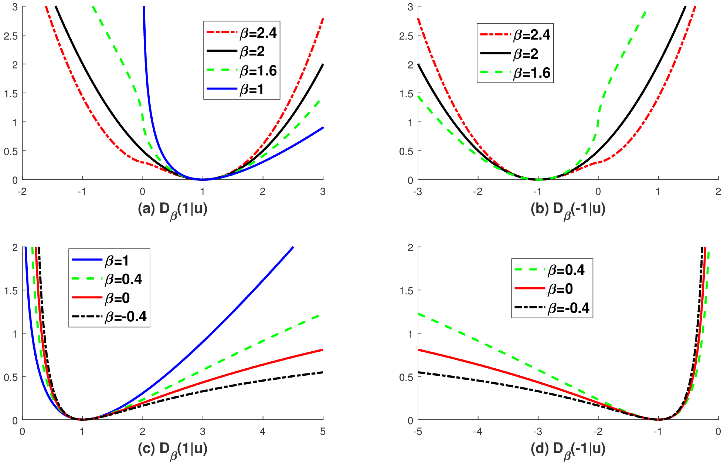
The graphs of the -divergence , which is based on the proposed extended logarithmic function in (4). (a) and (b) shows for with different choice of b, i.e., ; (c) and (d) shows for with different choice of b i.e., . Note that with is not defined if
Figure 1.
The graphs of the -divergence , which is based on the proposed extended logarithmic function in (4). (a) and (b) shows for with different choice of b, i.e., ; (c) and (d) shows for with different choice of b i.e., . Note that with is not defined if

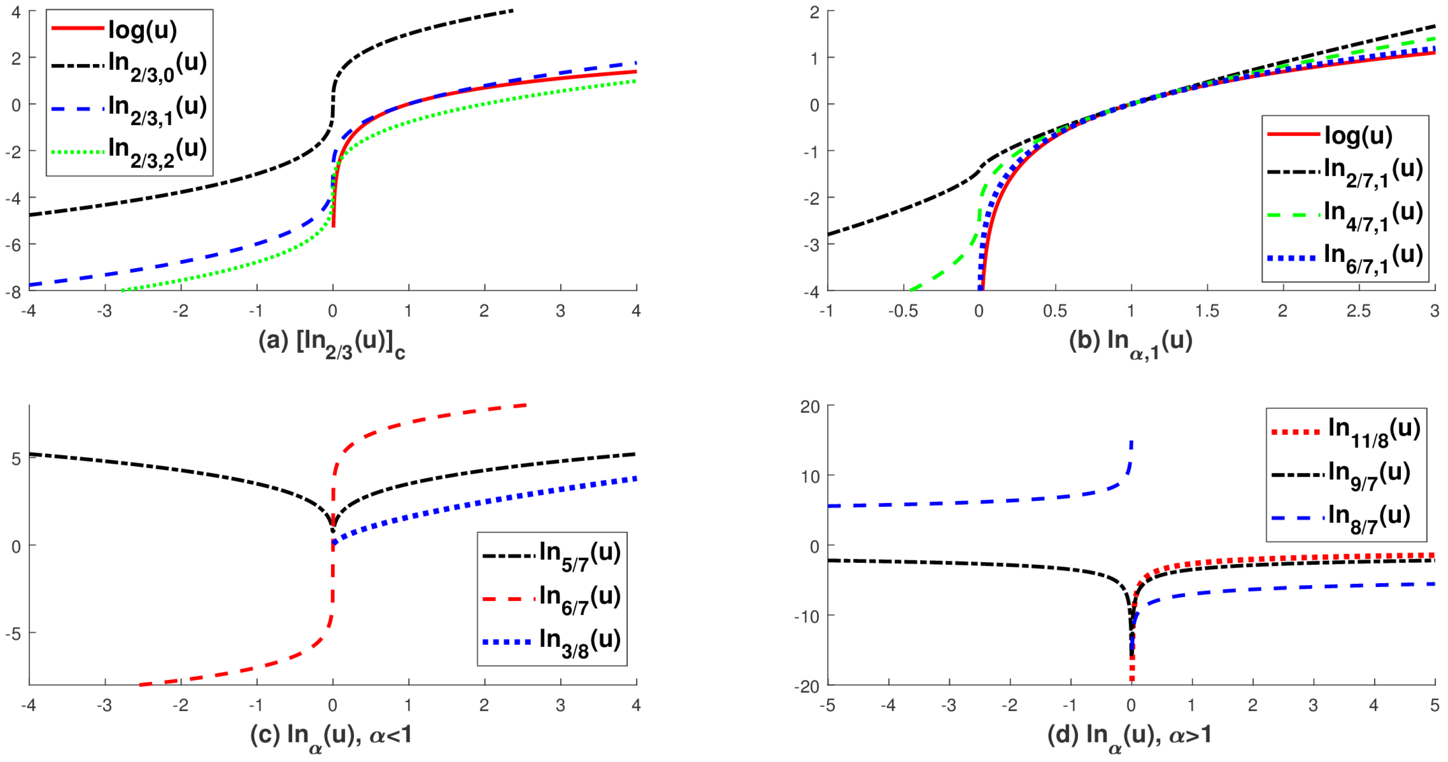
Figure 2.
The graphs of the extended logarithmic function in Definition 1. (a) shows an equivalence class with ; (b) shows with different choice of ; (c) and (d) show in (4) for different choices of . Note that is an extended logarithmic function without a constant term.
Figure 2.
The graphs of the extended logarithmic function in Definition 1. (a) shows an equivalence class with ; (b) shows with different choice of ; (c) and (d) show in (4) for different choices of . Note that is an extended logarithmic function without a constant term.

Table 1.
We compare the domain of the -divergence and the domain of the Bregman-divergence associated with the convex function of Legendre type in (19). We note that the domain () and the domain () do not exist in the Bregman-divergence. If we relax the Legendre condition of Φ as a convex and smooth function, then the Bregman-divergence also exists in the region with .
| Region | -Divergence | Bregman-Divergence | ||
|---|---|---|---|---|
| entire | ||||
| - | - | |||
| positive | and | |||
| negative | and | |||
Table 2.
The domain and range of the extended logarithmic function defined in (4).
Table 2.
The domain and range of the extended logarithmic function defined in (4).
| or | or | ||||||
| or |
Table 3.
A classification of the domain of the -divergence in terms of .
| and | |
| and | |
| and | |
| and | or |
| and | |
| and | or |
© 2017 by the author. Licensee MDPI, Basel, Switzerland. This article is an open access article distributed under the terms and conditions of the Creative Commons Attribution (CC BY) license (http://creativecommons.org/licenses/by/4.0/).
Share and Cite
MDPI and ACS Style
Woo, H. A Characterization of the Domain of Beta-Divergence and Its Connection to Bregman Variational Model. Entropy 2017, 19, 482. https://doi.org/10.3390/e19090482
AMA Style
Woo H. A Characterization of the Domain of Beta-Divergence and Its Connection to Bregman Variational Model. Entropy. 2017; 19(9):482. https://doi.org/10.3390/e19090482
Chicago/Turabian StyleWoo, Hyenkyun. 2017. "A Characterization of the Domain of Beta-Divergence and Its Connection to Bregman Variational Model" Entropy 19, no. 9: 482. https://doi.org/10.3390/e19090482
Note that from the first issue of 2016, this journal uses article numbers instead of page numbers. See further details here.