On Generalized Stam Inequalities and Fisher–Rényi Complexity Measures


1
GIPSA-Lab, Université Grenoble Alpes, 11 rue des Mathématiques, 38420 Grenoble, France
2
Instituto Carlos I de Física Teórica y Computacional, Universidad de Granada, 18071 Granada, Spain
3
Departamento de Física Atómica, Molecular y Nuclear, Universidad de Granada, 18071 Granada, Spain
*
Author to whom correspondence should be addressed.
Entropy 2017, 19(9), 493; https://doi.org/10.3390/e19090493
Submission received: 21 August 2017
/
Revised: 8 September 2017
/
Accepted: 12 September 2017
/
Published: 14 September 2017
(This article belongs to the Special Issue Foundations of Quantum Mechanics)
Abstract
:Information-theoretic inequalities play a fundamental role in numerous scientific and technological areas (e.g., estimation and communication theories, signal and information processing, quantum physics, …) as they generally express the impossibility to have a complete description of a system via a finite number of information measures. In particular, they gave rise to the design of various quantifiers (statistical complexity measures) of the internal complexity of a (quantum) system. In this paper, we introduce a three-parametric Fisher–Rényi complexity, named -Fisher–Rényi complexity, based on both a two-parametic extension of the Fisher information and the Rényi entropies of a probability density function characteristic of the system. This complexity measure quantifies the combined balance of the spreading and the gradient contents of , and has the three main properties of a statistical complexity: the invariance under translation and scaling transformations, and a universal bounding from below. The latter is proved by generalizing the Stam inequality, which lowerbounds the product of the Shannon entropy power and the Fisher information of a probability density function. An extension of this inequality was already proposed by Bercher and Lutwak, a particular case of the general one, where the three parameters are linked, allowing to determine the sharp lower bound and the associated probability density with minimal complexity. Using the notion of differential-escort deformation, we are able to determine the sharp bound of the complexity measure even when the three parameters are decoupled (in a certain range). We determine as well the distribution that saturates the inequality: the -Gaussian distribution, which involves an inverse incomplete beta function. Finally, the complexity measure is calculated for various quantum-mechanical states of the harmonic and hydrogenic systems, which are the two main prototypes of physical systems subject to a central potential.
1. Introduction
The definition of complexity measures to quantify the internal disorder of physical systems is an important and challenging task in science, basically because of the many facets of the notion of disorder [1,2,3,4,5,6,7,8,9,10,11,12]. It seems clear that a unique measure is unable to capture the essence of such a vague notion. In the scalar continuous-state context we consider in this paper, many complexity measures based on the probability distribution describing a system have been proposed in the literature, attempting to capture simultaneously the spreading (global) and the oscillatory (local) behaviors of such a distribution [10,12,13,14,15,16,17,18,19,20,21,22,23,24,25,26,27,28,29]. They mostly depend on entropy-like quantities such as the Shannon entropy [30], the Fisher information [31] and their generalizations. The measures of complexity of a probability density proposed up until now, say , making use of two information-theoretic properties, share several properties (see e.g., [32]), such as e.g., the invariance by translation or by a scaling factor (i.e., for any and , for they satisfy ). For instance, the disorder may be invariant from a move of a (referential independent) center of mass. Moreover, all the proposed measures are also lowerbounded, which means that there exists in a certain sense a distribution of minimal complexity, which is the probability density that reaches the lower bound.
In this paper, we generalize the complexity measures of global-local character published in the literature (see e.g., [10,12,23,24,26,27,29]) to grasp both the spreading and the fluctuations of a probability density by the introduction of a three-parametric Fisher–Rényi complexity, which involves the Rényi entropy [33] and generalized Fisher information [34,35,36]. The products of these two generalized information-theoretic tools, which are translation and scaling invariant as well as lowerbounded, can be used as generalized complexity measures of .
Historically, the first inequality involving the Shannon entropy and the Fisher information was proved by Stam [37] under the form
where F and N are, respectively, the (nonparametric) Fisher information of ,
and the Shannon entropy power of , i.e., an exponential of the Shannon entropy H,
In fact, the Fisher information concerns a density parametrized by a parameter and the derivative is vs. . When this parameter is a position parameter, this leads to the nonparametric Fisher information. Concerning the entropy power, more rigorously, a factor affects N and the bound in the Stam inequality is then unity. This factor does not change anything for our purpose, hence, for sake of simplicity, we omit it. The lower bound in Inequality (1) is achieved for the Gaussian distribution up to a translation and a scaling factor (where ∝ means “proportional to”). In other words, the so-called Fisher–Shannon complexity , which is translation and scale invariant, is always higher than (and thus cannot be zero) and the distribution of lowest complexity is the Gaussian, exhibiting (also) through this measure its fundamental aspect. The proof of this inequality lies in the entropy power inequality and on the de Bruijn identity, two information theoretic inequalities, both being reached in the Gaussian context [37,38].
Although introduced respectively in the estimation context through the Cramér–Rao bound [31,39,40] and in communication theory through the coding theorem of Shannon [30,38], these quantities found applications in physics as previously mentioned (and also in the earlier papers [41,42] and that of Stam). In particular, the analysis of a signal with these measures was proposed by Vignat and Bercher [43] and the Fisher–Shannon complexity is widely applied in atomic physics or quantum mechanics for instance [25,26,44,45,46,47].
Recently, the Stam inequality was extended by substituting the Shannon entropy by the Rényi entropies (a family of entropies characterizing by a parameter playing a role of focus [33]), and the Fisher information by a generalized two-parametric family of the Fisher information introduced by [34,35,36]. As we will see later on, this extended inequality involves, however, two free parameters because one of the two Fisher parameters is linked to the Rényi one. This constraint is imposed so as to determine the sharp bound of the inequality and the minimizers in the framework of the (stretched) Tsallis distributions [48,49]. Thus, this extended inequality allows to define again a complexity measure, based on this generalized Fisher information and the Rényi entropy power [27].
In this paper, we study the full three-parametric Fisher–Rényi complexity, disconnecting the two parameters tuning the extended Fisher information and the parameter tuning the Rényi entropy. Like Bercher, we use an approach based on the Gagliardo–Nirenberg inequality. This inequality allows for proving the existence of a lower bound of the complexity when the parameters are decoupled, in a certain range. The minimizers are thus implicitly known as a solution of a nonlinear equation (or through a complicated series of integrations and inversion of nonlinear functions). Moreover, the sharp bound of the associated extended Stam inequality is explicitly known, once the minimizers have been determined. We propose here an indirect approach allowing (i) to extend a step further the domain where the Stam inequality holds (or where the complexity is non trivially lower-bounded); (ii) to determine explicitly the minimizers; and (iii) to find the sharp bound, regardless of the knowledge of the minimizers.
The structure of the paper is the following. In Section 2, we introduce both the -dependent Rényi entropy power and the -Fisher information, so generalizing the usual (i.e., translationally invariant) Fisher information. Then, we propose a complexity measure based on these two information quantities, the -Fisher–Rényi complexity, and we study its fundamental properties regarding the invariance under translation and scaling transformations and, above all, the universal bounding from below. In particular, we come back briefly to the results of Lutwak [34] or of Bercher [35] concerning the sharpness of the bound and the minimizers, derived only when the three parameters belong to a two-dimensional manifold, finding that our results remain indeed valid in a domain slightly wider than theirs. In Section 3, the core of the paper, we come back to the lower bound (or to the extended Stam inequality) dealing with a wide three-dimensional domain. In this extended domain, which includes that of the previous section, we are able to derive explicitly the minimizers and the sharp lower bound, regardless the knowledge of the minimizers. In order to do this, we introduce a special nonlinear stretching of the state, leading to the so-called differential-escort distribution [50]. This geometrical deformation allows us to start from the Bercher–Lutwak inequality and to introduce a supplementary degree of freedom so as to decouple the parameters (in a certain range). This approach is the key point for the determination of the extended domain where the complexity is bounded from below (the generalized Stam inequality). Moreover, we provide an explicit expression for the densities which minimize this complexity, expression involving the inverse incomplete beta function. In Section 4, we apply the previous results to some relevant multidimensional physical systems subject to a central potential, whose quantum-mechanically allowed stationary states are described by wave functions that factorize into a potential-dependent radial part and a common spherical part. Focusing on the radial part, we calculate the three-parametric complexity of the two main prototypes of d-dimensional physical systems, the harmonic (i.e., oscillator-like) and hydrogenic systems, for various quantum-mechanical states and dimensionalities. Finally, three appendices containing details of the proofs of various propositions of the paper are reported.
2. -Fisher–Rényi Complexity and the Extended Stam Inequality
In this section, we firstly review the extension of the Stam inequality based on the efforts of Lutwak et al. and Bercher [34,35,36], or more generally, based on that of Agueh [51,52]. To this aim, we introduce a three-parametric Fisher–Rényi complexity, showing its scaling and translation invariance and non-trivial bounding from below. We then come back to the results of Lutwak or Bercher concerning the determination of the sharp bound and the minimizers of its associated complexity, where a constraint on the parameters was imposed. Indeed, the constraint they imposed can be slightly relaxed, as we will see in this section.
2.1. Rényi Entropy, Extended Fisher Information and Rényi–Fisher Complexity
Let us begin with the definitions of the following information-theoretic quantities of the probability density : the Rényi entropy power , the -Fisher information , and the -Fisher–Rényi complexity .
Definition 1
(Rényi entropy power [33]). Let . Provided that the integral exists, the Rényi entropy power of index λ of a probability density function ρ is given by
where the limiting case gives the Shannon entropy power .
The entropy was introduced by Rényi in [33] as a generalization of the Shannon entropy. In this expression, through the exponent applied to the distribution, more weight is given to the tail () or to the head () of the distribution [34,53,54,55]. This measure found many applications in numerous fields such as e.g., signal processing [56,57,58,59,60,61,62], information theory to reformulate the entropy power inequality [63], statistical inference [64], multifractal analysis [65,66], chaotic systems [67], or in physics as mentioned in the introduction (see ref. above). For instance, the Rényi entropies were used to reformulate the Heisenberg uncertainty principle (see [68,69,70,71,72] or [73,74] where this formulation also appears and is applied in quantum physics).
Whereas the power applied to the probability density in the Rényi entropy aims at making a focus on heads or tails of the distribution, one may wish to act similarly dealing with the Fisher information. In this case, since both the density and its derivative are involved, one may wish to stress either some parts of the distribution, or some of its variations (small or large fluctuations). Thus, two different power parameters for and its derivative, respectively, can be considered leading with our notations to the following definition of the bi-parametric Fisher information.
Definition 2
(-Fisher information [34,35,36]). For any and any , the -Fisher information of a continuously differentiable density ρ is defined by
provided that this integral exists. When ρ is strictly positive on a bounded support, the integration is to be understood over this support, but it must be differentiable on the closure of this support.
It is straightforward to see that is the usual Fisher information. When it exists, is the essential supremum of . Conversely, is the total variation of . For , this extended Fisher information is closely related to the -Fisher information introduced by Hammad in 1978 when dealing with a position parameter [75]. Note also that a variety of generalized Fisher information was applied especially in non-extensive physics [76,77,78,79].
From the Rényi entropy power and the -Fisher information, we define a -Fisher–Rényi complexity by the product of these quantities, up to a given power.
Definition 3
(-Fisher–Rényi complexity). We define the -Fisher–Rényi complexity of a probability density ρ by
provided that the involved quantities exist.
We choose to elevate the product of the entropy power and Fisher information to the power for simplification reasons. Indeed, it does not change the spirit of this measure of complexity, whereas it allows to express symmetry properties in a more elegant manner, as we will see later on.
This quantity has the minimal properties expected for a complexity measure (see e.g., [32]), as stated in the next subsection.
2.2. Shift and Scale Invariance, Bounding from Below and Minimizing Distributions
The first property of the proposed complexity is the invariance under the basic translation and scaling transformations.
Proposition 1.
The -Fisher–Rényi complexity of the probability density ρ is invariant under any translation and scaling factor applied to ρ; i.e., for .
Proof.
This is a direct consequence of a change of variables in the integrals, showing that (justifying the term of entropy power) for any , and that , whatever . ⎕
From now, due to these properties, all the definitions related to probability density functions will be given up to a translation and scaling factor. In other words, when evoking a density , except when specified, we will deal with the family for any and .
More important, the complexity has a universal, non-trivial bounding from below so that the distribution corresponding to this minimal complexity can thus be viewed as the less complex one.
Proposition 2
(Extended Stam inequality). For any ,
with the Holder conjugate of p, their exists a universal optimal positive constant , that bounds from below the -Fisher–Rényi complexity of any density ρ, i.e.,
The optimal bound is achieved when, up to a shift and a scaling factor,
and where u is a solution of the differential equation
with γ determined a posteriori to impose that sums to unity. When , the limit has to be taken, leading to .
Proof.
The proof is mainly based on the sharp Gagliardo–Nirenberg inequality [52], as explained with details in Appendix A. ⎕
Finally, the minimizers of the -Fisher–Rényi complexity and the tight bound satisfy a remarkable property of symmetry, as stated hereafter.
Proposition 3.
Let us consider the involutary transform
The minimizers of the complexity satisfy the relation
and the optimal bounds satisfy the relation
Proof.
See Appendix B. ⎕
A difficulty to determine the sharp bound and the minimizer is to solve the nonlinear differential Equation (10). One can find in Corollary 3.2 in [52] a series of explicit equations allowing to determine the solution and thus the optimal bound of in Equation (A1), but in general the expression of u remains on an integral form. Agueh, however, exhibits several situations where the solution is known explicitly (and thus the optimal bound as well), as summarized in the next subsection.
2.3. Some Explicitly Known Minimizing Distributions
The particular cases are issued of special cases of saturation of the Gagliardo–Nirenberg, some of them being studied by Bercher [35,80,81] or Lutwak [34]. All these cases are restated hereafter, with the notations of the paper. Let us first recall the definition of the stretched deformed Gaussian, studied by Lutwak [34] or Bercher [35,80,81], for instance, also known as stretched q-Gaussian or stretched Tsallis distributions [48,49] and intensively studied in non-extensive physics.
Definition 4
(Streched deformed Gaussian distribution). Let and . The -stretched deformed Gaussian distribution is defined by
where (the case is indeed obtained taking the limit).
This distribution plays a fundamental role in the extended Stam inequality, as we will see in the next subsections and in the next section.
2.3.1. The Case
For any , and for
one obtains that the minimizing distribution of the -Fisher–Rényi complexity is the -stretched deformed Gaussian distribution,
(see Corollary 3.4 in [52], (i) where ; and (ii) where , respectively; the case is obtained taking the limit (resp. lower and upper limit) or by a direct computation). This situation is nothing more than that studied by Bercher in [35] or Lutwak in [34]. Remarkably, by a mass transport approach, Lutwak proved in [34] that this relation is valid for , i.e., for
Note that the exponent of the Lutwak expression is not the same as ours, but allowing to take the Lutwak relation to the adequate exponent so as to obtain our formulation.
2.3.2. Stretched Deformed Gaussian: The Symmetric Case
Immediately, from the relation Equation (12) induced by the involution , one obtains, after a re-parametrization and an adequate scaling, for any and
that the minimizing distribution is again a stretched deformed Gaussian,
Again, starting from the Lutwak result, the validity of this result extends to
and the symmetry of the bound given by Proposition 3 remains valid. Indeed, the minimizers in satisfying the differential equation of the Gagliardo–Nirenberg as given in Appendix A, the reasoning of this appendix and of the Appendix B holds.
2.3.3. Dealing with the Usual Fisher Information
This situation corresponds to and . Then, for
one obtains the minimizing distribution for ,
where denotes the indicator function of set A, (remember that ), is the real part and is to be understood as (see Corollary 3.3 in [51] with and Corollary 3.4 in [51] with respectively). The case is again obtained by taking the limit, leading to the Gaussian distribution . (See previous cases, with , that corresponds also to the usual Stam inequality.)
2.3.4. The Symmetrical of the Usual Fisher Information
From the relation Equation (12) induced by the involution , after a re-parametrization and an adequate scaling, for and
the minimizing distribution for takes the form
(with, again, the Gaussian as the limit when ).
3. Extended Optimal Stam Inequality: A Step Further
In this section, we further extend the previous Stam inequality, namely by largely widening the domain for the parameters and disentangling the two connected parameters. For this, we use the differential-escort deformation introduced in [50], which is the key tool allowing for introducing a new degree of freedom. Afterwards, we will give the minimizing distribution that results in a new deformation of the Gaussian family intimately linked with the inverse incomplete beta functions.
3.1. Differential-Escort Distribution: A Brief Overview
We have already realized the crucial role that the power operation of a probability density function plays. The subsequent escort distribution duly normalized, , is a simple monoparametric deformation of (see e.g., [82]). Notice that the parameter allows us to explore different regions of , so that, for , the more singular regions are amplified and, for , the less singular regions are magnified. A careful look at the minimizing distributions of the usual Stam inequality shows that the x-axis is stretched via a power operation. This makes us guess that a certain nonlinear stretching may also play a key role in the saturation (i.e., equality) of the extended Stam inequality.
These ideas led us to the definition of the differential-escort distribution of a probability distribution (see also [50]), motivated by the following principle. The power operation provokes a two-fold stretching in the density itself and in the differential interval so as to conserve the probability in the differential intervals: with .
Definition 5
(Differential-escort distributions). Given a probability distribution and given an index , the differential-escort distribution of ρ of order α is defined as
where is a bijection satisfying and .
The differential-escort transformation exhibits various properties studied in detail in [50]. We present here the key ones, allowing the extension of the Stam inequality in a wider domain than that of the previous section.
Property 1.
The differential-escort transformation satisfies the composition relation
where ∘ is the composition operator. Moreover, since is the identity, for any , is invertible and,
In addition to the trivial case , keeping invariant the distribution, a remarkable case is given by , leading to the uniform distribution. This case is non surprising since then is nothing more than the inverse of the cumulative density function, well known to uniformize a random vector [83].
In the sequel, we focus on the differential-escort distributions obtained for . Under this condition, when is continuously differentiable, its differential-escort is also continuously differentiable. This is important to be able to define its -Fisher information (see Definition 2). Under this condition, the differential-escort transformation induces a scaling property on the index of the Rényi entropy power (for this quantity it remains true for any ), the -Fisher information, and thus on the subsequent complexity as stated in the following proposition.
Proposition 4.
Let a probability distribution ρ and an index . Then, the Rényi entropy powers of ρ and its differential-escort distribution satisfy that
for any . Moreover, if the density ρ is continuously differentiable, then the extended Fisher information of ρ and its differential-escort distribution satisfy that
for any .
Consequently, the -Fisher–Rényi complexity of ρ and of satisfy the relation
One may mention [84] where the author studies the effect of a rescaling of the Tsallis non-additive parameter, equivalent to the entropic parameter of the Rényi entropy, and that is exactly that of Equation (28). In particular, this rescaling has an effect on the maximum entropy distribution in such a way that it is equivalent to elevate this particular distribution to a power. Here, the spirit is slightly different since we start from a given distribution and the nonlinear stretching is made on the state (x-axis) of any probability density in such a way that it is elevated to an exponent. The stretching is intimately linked to the distribution, being of maximum entropy or not, and the scaling effect on the Rényi is a consequence of this nonlinear stretching. The study of the links between the present result and that of [84] goes beyond the scope of our work and remains as a perspective.
3.2. Enlarging the Validity Domain of the Extended Stam Inequality
We have now all the ingredients to enlarge the domain of validity of the Stam inequality. Moreover, we are able to determine an explicit expression of the minimizer by the mean of a special function, i.e., more simple to determine than as in Proposition 2, and of the tight bound as well.
To this aim, let us consider the following affine transform and the set of transformation for ,
Then, for any strictly positive real a, one can apply Proposition 2 to , that is, for , , . Thus, from Proposition 4, one immediately has that . Moreover, this inequality is sharp since it is achieved for , i.e., for .
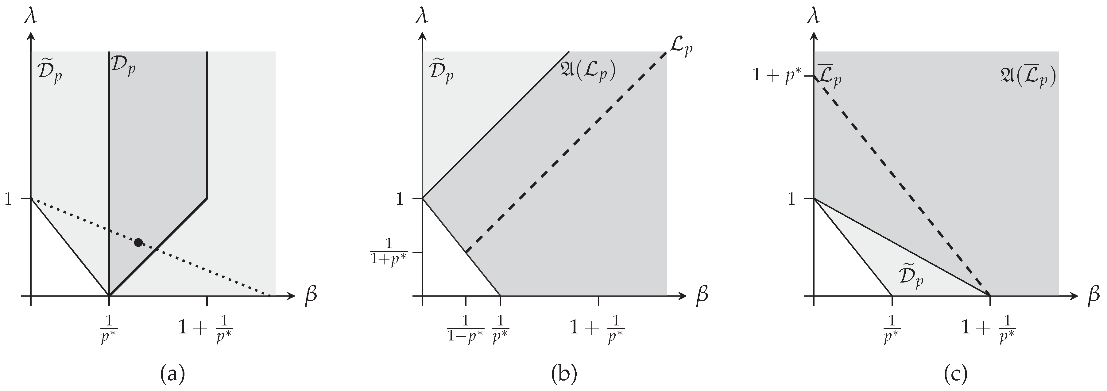
As a conclusion, the existence of a universal optimal positive constant bounding the complexity (see Proposition 2) extends from to . Note that is the overlap of the line defined by the point and itself (achieved for ), and , as depicted Figure 2. Then, it is straightforward to see that (see Figure 2a). The approach is thus the following:
- Consider a point and find an index such that , which is a point of the intersection between and the line joining and .
- Apply Proposition 2 for the point , leading to the minimizing distribution and its corresponding bound.
- Then, remarking that , the minimizer of the extended complexity writes and the corresponding bound can be computed from this minimizer or noting that .
The same procedure obviously applies dealing with : appears to be a subset of (see Figure 2b). Similarly, one can also deal with : also appears to be a subset of (see Figure 2c). Remarkably, . Moreover, we have explicit expressions for the minimizers in both and , which greatly eases determining the minimizers in (including itself).
These remarks, together with both the knowledge of the minimizing distributions and the bound on , lead to the following definition and proposition.
Definition 6
(-Gaussian distribution). For any and , we define the -Gaussian distribution as
with
is the involutary transform defined Equation (11). is the incomplete beta function, defined when and for (see [85]), and , that is the standard beta function if and infinite otherwise. is thus the inverse incomplete beta function. Finally, is the incomplete gamma function, defined when and for [85], and is the gamma function. By definition, where . Finally, by convention .
Note that, when , the inverse incomplete beta function is well known and tabulated in the usual mathematical softwares since it is the inverse cumulative function of the beta distributions [86]. Otherwise, as the incomplete beta function writes through an hypergeometric function [87] (see also [85,86]), also well known and tabulated, can be at least numerically computed. The incomplete beta function contains many special cases for particular parameters [87,88]. For instance, when is a negative integer, they express as elementary functions [87].
Similarly, when its argument is positive, the incomplete gamma function and its inverse are well known and tabulated because they are linked to the cumulative distribution of gamma laws [86]. Even for negative arguments, the incomplete gamma function is very often tabulated in mathematical software. Otherwise, one can write it using a confluent hypergeometric function [85] (see also [86,87]), generally tabulated. Thus, it can be inverted at least numerically. The incomplete gamma function also contains special cases for particular parameters. For instance, where erf is the error function [85]. Hence, for and , the -Gaussian writes in terms of the inverse error function.
Now, from the procedure previously described, we obtain the Stam inequality with the widest possible domain, together with the minimizing distributions and the explicit tight lower bound.
Proposition 5
(Stam inequality in a wider domain). The -Fisher–Rényi complexity is non trivially lower bounded as follows:
The minimizers are explicitly given by
the -Gaussian of Definition 6. Proposition 3 remains valid in . Moreover, the tight bound is
with
Proof.
See Appendix C. ⎕
4. Applications to Quantum Physics
Let us now apply the -Fisher–Rényi complexity for some specific values of the parameters to the analysis of the two main prototypes of d-dimensional quantum systems subject to a central (i.e., spherically symmetric) potential; namely, the hydrogenic and harmonic (i.e., oscillator-like) systems. The wave functions of the bound stationary states of these systems have the same angular part, so that we concentrate here on the radial distribution in both position and momentum spaces.
4.1. Brief Review on the Quantum Systems with Radial Potential
The time-independent Schrödinger equation of a single-particle system in a central potential can be written as
(atomic units are used from here onwards), where denotes the d-dimensional gradient operator and the position vector in hyperspherical units is given by , the unit d-dimensional sphere, where and for and with for , and by convention. The physical wave functions are known to factorize (see e.g., [89,90,91]) as
where and denote the radial and the angular part, respectively, being the hyperquantum numbers associated to the angular variables , which may take all values consistent with the inequalities .
As already stated, the angular part is independent of the potential V and its expression is detailed in [14,17,91,92], for instance. Only the radial part is dependent on V (and also on the energy level n and the angular quantum number l), being the solution of the radial differential equation
(see e.g., [14,17,92] for further details). Then, the associated radial probability density is given by
where we have taken into account the volume element and the normalization of the hyperspherical harmonics to unity.
Then, the wavefunction associated to the momentum of the system is given by the Fourier transform of . It is known that, again, writes as the product of a radial and angular part
with the the radial part being the modified Hankel transform of ,
with the Bessel function of the first king and order (see e.g., [14,17,91,92]). Again, it leads to the radial probability density function
In the following, we will focus on the -Fisher–Rényi complexity of the radial densities and of the d-dimensional harmonic and hydrogenic systems.
4.2. -Fisher–Rényi Complexity and the Hydrogenic System
The bound states of a d-dimensional hydrogenic system, where (Z denotes the nuclear charge) are the physical solutions of Equation (40), which correspond to the known energies
(see [14,89,90]). The radial eigenfunctions are given by
L is the grand orbital angular momentum quantum number, is a dimensionless parameter, and the normalization coefficient are given by
respectively, with the Laguerre polynomials [85,87]. Then, the radial probability density (41) of a d-dimensional hydrogenic stationary state is given in position space by
Furthermore, using 8.971 in [87], one can compute .
On the other hand, the modified Hankel transform of Equation (43) gives the radial part of the wavefunction in the conjugated momentum space as [14,89,90]
where is a dimensionless parameter and the normalization coefficient are given by
and where denotes the Gegenbauer polynomials [85,87]. This gives the radial probability density function in the momentum space as
Furthermore, using 8.939 in [87], one can compute .
These expressions can thus be injected into Equations (4)–(6) to evaluate the -Fisher–Rényi complexity of both and . Due to the special form of the density, involving orthogonal polynomials, this can be done using for instance a Gauss-quadrature method for the integrations [86].
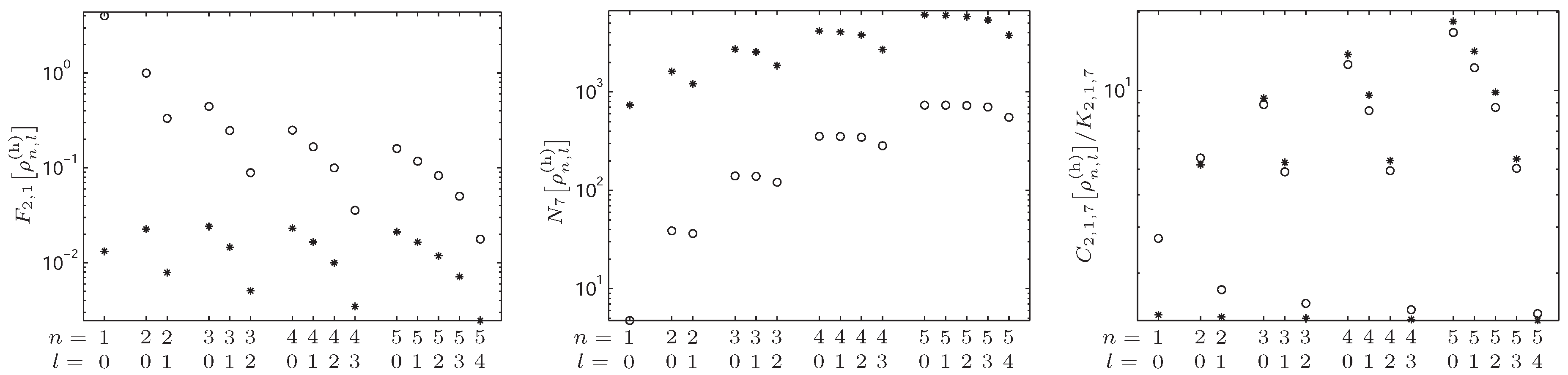
For illustration purposes, we depict in Figure 3 the behavior of the Fisher information , of the Rényi entropy power , and of the -Fisher–Rényi complexity (normalized by the lower bound) of the radial position density of the d-dimensional hydrogenic system, versus n and l, for the parameters and in dimensions and 12. Therein, we firstly observe that, for a given quantum state of the system (so, when n and l are fixed), the Fisher information decreases (see left graph) and the Rényi entropy power increases (see center graph) when d goes from 3 to 12. This indicates that the oscillatory degree and the spreading amount of the radial electron distribution have a decreasing and increasing behavior, respectively, when the dimension is increasing. The resulting combined effect, as captured and quantified by the the Fisher–Rényi complexity (see right graph), is such that the complexity has a clear dependence on the difference in such a delicate way that it decreases when but it increases when is bigger than unity as d is increasing.
To better understand this phenomenon, we have to look carefully at the opposite behavior of the Fisher information and the Rényi entropy power versus the pair .
Indeed, for the two dimensionality cases considered in this work, the Fisher information presents a decreasing behavior when l is increasing and n is fixed, reflecting essentially that the number of oscillations of the radial electron distribution is gradually smaller; keep in mind that is the degree of the Laguerre polynomials which controls the radial electron distribution. At the smaller dimension (), a similar behavior is observed when l is fixed and n is increasing, while the opposite behavior occurs at the higher dimension (). This indicates that the radial fluctuations are bigger in number as n increases and their amplitudes depend on the dimension d so that they are gradually smaller (bigger) at the high (small) dimension. This is because the dimension, hidden in both the hyperquantum numbers and L, tunes the coefficients of the Laguerre polynomials and thus the amplitude height of the oscillations.
In the case of the Rényi quantity, which is a global spreading measure, the behavior for fixed l and n increasing is clearly increasing, whereas, for fixed n, it is slowly decreasing versus l; this indicates that the radial electron distribution gradually spreads more and more (less and less) all over the space when is increasing.
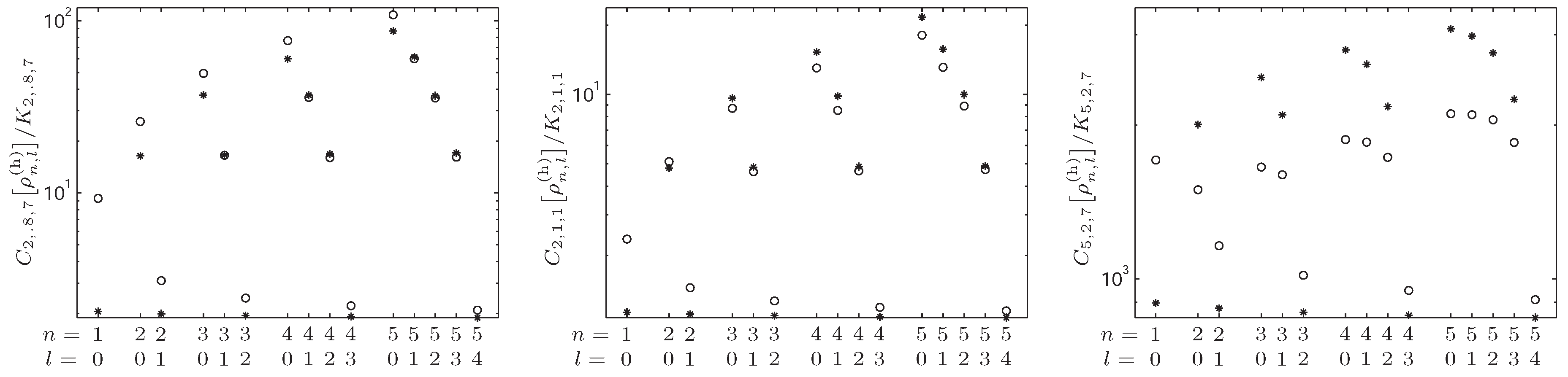
Then, in Figure 4, the parameter dependence of the -Fisher–Rényi complexity (duly normalized to the lower bound) for the radial distribution of various states of the d-dimensional hydrogenic system in position space with dimensions and 12, is investigated for the sets , (usual Fisher–Shannon complexity) and . Roughly speaking, the average behavior of the complexity versus is similar for both dimensional cases to the one shown in the right graph of the previous figure. Of course, for a given pair (), the behavior of the complexity in terms of the dimension is quantitatively different according to the values of the parameters. Let us just point out, for instance, that the comparison of the behavior of versus d and the corresponding ones of the other complexities shows that the complexity with higher value of p is more sensitive to the radial electron fluctuations with higher amplitudes.
A similar study for the previous entropy- and complexity-like measures in momentum space has been done in Figure 5 and Figure 6. Briefly, we observe that the behavior of these momentum quantities are in accordance with the analysis of the corresponding ones in position space, which has just been discussed. Note that here again the difference determines the degree of the Gegenbauer polynomials that control the momentum density , so that the influence of and d is formally similar to that for the position density . Here, the influence of d on the height of the radial oscillation of the electron distribution (through the coefficients of the Gegenbauer polynomials) is the same for the two dimensionality cases considered in this work.
Let us highlight that the -behavior of the Rényi power entropy in momentum space is just the opposite to the corresponding position one, manifesting the conjugacy of the two spaces, which is the spread of the position and momentum electron distributions are opposite.
4.3. -Fisher–Rényi Complexity and the Harmonic System
The bound states of a d-dimensional harmonic (i.e., oscillator-like) system, where (without loss of generality, the mass is assumed to be unity), are known to have the energies
(see e.g., [90,93,94]). The radial eigenfunctions writes in terms of the Laguerre polynomials as
where is a dimensionless parameter, and the normalization coefficient are given by
respectively. Then, the associated radial position density is thus given by
As for the hydrogenic system, using 8.971 in [87], one can compute , and thus the -Fisher–Rényi of . Remarkably, is invariant by the modified Hankel transform, so that the momentum radial density is formally the same as the position radial density.
For illustration purposes, we plot in Figure 7 the behavior of the Fisher information , the Rényi entropy power and the -Fisher–Rényi complexity of the radial position distribution of the d-dimensional harmonic system for various values of the quantum numbers n and l at the dimensions and 12. Figure 8 depicts duly renormalized by its lower bound, for the triplets of complexity parameters and , respectively. In these graphs, one can make a similar interpretation as for the hydrogenic case. Note, however, that here the degree of the Laguerre polynomials involved in the distribution only depends on n; this fact makes more regular the behavior of the previous information-theoretical measures in the oscillator case than in the hydrogenic one. Concomitantly, as n increases, the spreading of the distribution also increases. Conversely, parameters l and d have a relatively small influence on both the smoothness of the oscillation and on the spreading (compared to that of n). Thus, unsurprisingly, both the Fisher information and the Rényi entropy power are weakly influenced by l (especially at the higher dimension) and by d. The Fisher–Rényi complexity, which quantifies the combined oscillatory and spreading effects, exhibits a very regular increasing behavior in terms of n.
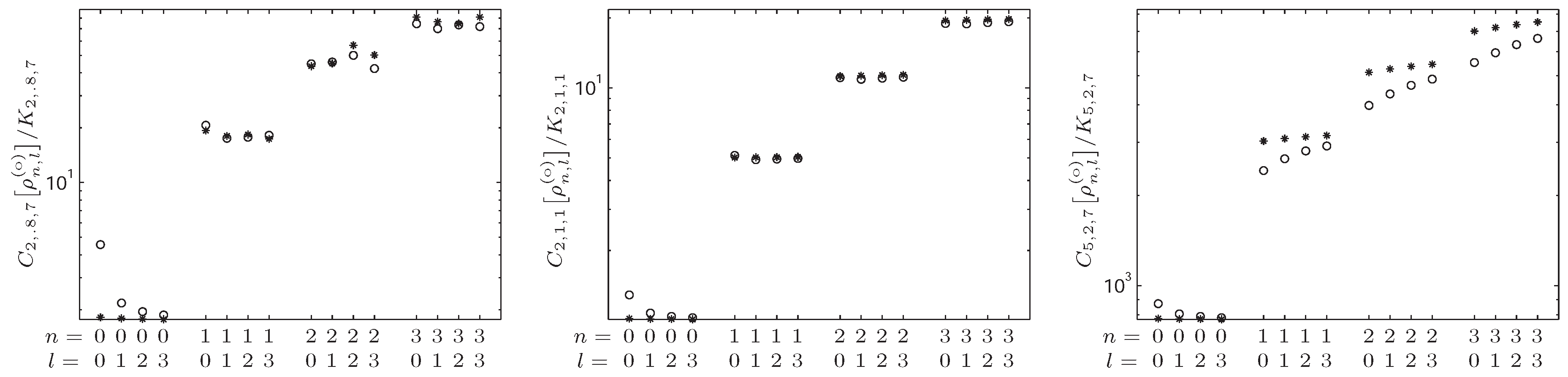
Most interesting is the parameter-dependence of the complexity. Indeed, we can play with the complexity parameter to stress different aspects of the oscillator density and thus to reveal differences between the quantum states of the system. For instance, as one can see in Figure 8, the usual Fisher–Rényi complexity is unable to quantify the difference between the states of a given n versus the orbital number l and the dimension d (especially when , whereas the systems are quite different). This holds even playing with or , while increasing parameter p (right graph), these states are distinguishable. This graph clearly shows the potentiality of the family of complexities to analyze a system, especially thanks to the full degree of freedom we have between the complexity parameters and .
5. Conclusions
In this paper, we have defined a three-parametric complexity measure of Fisher–Rényi type for a univariate probability density that generalizes all the previously published quantifiers of the combined balance of the spreading and oscillatory facets of . We have shown that this measure satisfies the three fundamental properties of a statistical complexity, namely, the invariance under translation and scaling transformations and the universal bounding from below. Moreover, the minimizing distributions are found to be closely related to the stretched Gaussian distributions. We have used an approach based on the Gagliardo–Nirenberg inequality and the differential-escort transformation of . In fact, this inequality was previously used by Bercher and Lutwak et al. to find a biparametric extension of the celebrated Stam inequality which lowerbounds the product of the Rényi entropy power and the Fisher information. We have extended this biparametric Stam inequality to a three-parametric one by using the idea of differential-escort deformation of a probability density.
Then, we have numerically analyzed the previous entropy-like quantities and the three-parametric complexity measure for various specific quantum states of the two main prototypes of multidimensional electronic systems subject to a central potential of Coulomb (the d-dimensional hydrogenic atom) and harmonic (the d-dimensional isotropic harmonic oscillator) character. Briefly, we have found that the proposed complexity allows to capture and quantify the delicate balance of the gradient and the spreading contents of the radial electron distribution of ground and excited states of the system. The variation of the three parameters of the proposed complexity allows one to stress differently this balance in the various radial regions of the charge distribution.
The results found in this work can be generalized in various ways that remain open. Indeed, the Gagliardo–Nirenberg relation is quite powerful since it involves the p-norm of the function u, the q-norm of its j-th derivative and the s-norm of its m-th derivative, where and the integers are linked by inequalities (see [95]). This leaves open the possibility to define still more extended (complete) complexity measures, with higher-order (in terms of derivative) measures of information. Even more interesting, this inequality-based relation holds for any dimension ; thus, it supports the possibility to extend our univariate results to multidimensional distributions, but with tighter restrictions on the parameters. The main difficulty in this case is related with the multidimensional extension of the validity domain by using the differential-escort technique or a similar one.
Acknowledgments
The authors are very grateful to the CNRS (Steeve Zozor) and the Junta de Andalucía and the MINECO–FEDER under the grants FIS2014–54497 and FIS2014–59311P (Jesús Sánchez-Dehesa) for partial financial support. Moreover, they are grateful for the warm hospitality during their stays at GIPSA–Lab of the University of Grenoble–Alpes (David Puertas-Centeno) and Departamento de Física Atómica, Molecular y Nuclear of the University of Granada (Steeve Zozor) where this work was partially carried out.
Author Contributions
The authors contributed equally to this work.
Conflicts of Interest
The authors declare no conflict of interest.
Appendix A. Proof of Proposition 2
Appendix A.1. The Case λ ≠ 1
The result of the proposition is a direct consequence of the Gagliardo–Nirenberg inequality [35,52,95], stated in our context as follows: let and ; then, there exists an optimal strictly positive constant K, depending only on and s such that for any function ,
provided that the involved quantities exist, the equality being achieved for u solution of the differential equation
where is such that is fixed and can be chosen arbitrarily (it corresponds to a Lagrange multiplier, see Equations (26) and (27) in [52]). Finding u thus allows to determine the optimal constant K. Note that, if the equality in (A1) is reached for , then it is also reached for for any . One can see that satisfies the differential equation . Thus, function u reaching the equality in Equation (A1) can also be chosen as the solution of the differential equation , where and can be chosen arbitrarily. As we will see later on, a judicious choice allowing to include the limit case is to take , i.e., to chose function u reaching the equality in Equation (A1) as the solution of the differential equation
where can be arbitrarily chosen.
Appendix A.1.1. The Sub-Case λ < 1
Following the very same steps than in [35], let us consider first
With integrable, one can normalize it, that is, writing it under the form with a probability density function. Thus, and from the Gagliardo–Nirenberg inequality,
Simple algebra allows to write the terms of the left-hand side in terms of the generalized Fisher information and of the Rényi entropy power, respectively, to conclude that
Using , let us then denote
and note that the conditions imposed on and s together with impose
once p and are given. Simple algebra allows thus to show that : the exponent of the Fisher information and of the entropy power in Equation (A4) are thus equal. Moreover, being strictly positive, both sides of Equation (A4) can be elevated to exponent leading to the result of the proposition, where the bound is given by
where s and can be expressed by their parametrization in . Finally, the differential Equation (10) satisfied by the minimizer u comes from Equation (A3) noting that and , remembering that and thus that is to be chosen such that sums to unity.
Appendix A.1.2. The Sub-Case λ > 1
Consider now
and , leading to
Denoting now
imposing
once p and are given. Simple algebras allows thus to show that : again, the exponent of the Fisher information and of the entropy power in Equation (A6) are equal. Here again, allowing to elevate both side of Equation (A6) to exponent . The bound is now given by
where q and can be expressed by their parametrization in . Finally, as for the previous case, the differential Equation (10) satisfied by the minimizer u comes from Equation (A3) noting that now and , remembering that now and thus that is to be chosen such that sums to unity.
Appendix A.2. The Case λ = 1
The minimizer for can be viewed as the limiting case , i.e., .
One can also process as done by Agueh in [52] to determine the sharp bound of the Gagliardo–Nirenberg inequality. To this end, let us consider the minimization problem
for and (see Chapters 5 and 6 in [96] justifying the existence of a minimum). Hence, there exists an optimal constant K such that for any function u such that sums to unity,
Now, fix a function u and consider for some . also sums to unity and thus can be put in the previous inequality, leading to
for any . Thus, this inequality is necessarily satisfied for the that minimizes . A rapid study of allows to conclude that it is minimum for
Now, injecting Equation (A11) in Equation (A10) gives
with . Consider now the minimizer of problem (A8). Obviously, is minimum for , that gives, from Equation (A11), and from Equation (A9), being an equality, . Injecting these expressions in Equation (A12) allows concluding that this inequality is sharp, and moreover that its minimizer coincides with that of the minimization problem (A8).
Inequality (8) is obtained by injecting in Equation (A12) and after some trivial algebra and denoting , confirming that it can be viewed as a limit case .
Let us now solve the minimization problem (A8), that is, from the Lagrangian technique [97], to minimize where and where and is the Lagrange multiplier. The solution of this variational problem is given by the Euler–Lagrange equation [97], , that writes here after a re-parametrization
is to be determined a posteriori so as to satisfy the constraint . Again, one can easily see that if the bound in Equation (A12) is achieved for , then it is also achieved for whatever . Reporting in the differential equation allows to see that is a solution of the differential equation . Choosing and rewriting , one can thus choose the minimizer u as the solution of the differential equation
where is to be determined a posteriori so as to satisfy the constraint . This result is precisely the limit case of the differential Equation (A3) when .
Appendix B. Proof of Proposition 3
Then, for , Relation (12) comes from the fact that the function u solution of Equation (A3) depends only on and s. Let us write and the parameters for the first situation of the above proof, i.e., and , and and the parameters for the second situation, i.e., and . It is straightforward to see that and , i.e., , and, conversely, that . Since the optimal u is fixed once and s are given, one has . Finally, simple algebra allows to show that and , which finishes the proof.
Appendix C. Proof of Proposition 5
Appendix C.1. The (p,β,λ)-Fisher–Rényi Complexity is Lowerbounded over
As detailed in the text, consider a point . Thus, there exists an index such that . Applying Propositions 2 and 4, we have
Appendix C.2. Explicit Expression for the Minimizers.
In the sequel, we determine the differential-escort transformation with . Let us denote by the normalization coefficient of the distribution [35,87]). Hence, as defined in Definition (5), with
Thus, writes
when making the change of variables and denoting . One can recognize in the integral the incomplete beta function defined when and for [85]. Here, , and noting that . Hence,
Note that , where is the beta function [85,86,87]; is thus infinite when .
Denoting the inverse of incomplete beta function, we obtain
and, thus,
Note that from [86,87]), we naturally recover that .
Finally, let us remark that
the first ensemble being a subset of and the second one a subset of . We treat now these three cases separately.
Appendix C.2.1. The Case 1 − p*β < λ < 1
Following Appendix C.1, let us first determine such that , which is such that . Hence,
The fact that and insures that .
From Section 2.3.1 and Appendix C.1, the minimizer of the complexity is thus given by
One can easily see that , and thus we immediately get from Equation (A17),
Noting that , it appears that this density is nothing more than the -Gaussian of Definition 6 (remember that the families of density are defined up to a shift and a scaling).
Appendix C.2.2. The Case λ > 1
Following again Appendix C.1, let us first determine such that , i.e., such that . We thus obtain
The fact that and insures that .
From Section 2.3.1 and Appendix C.1, the minimizers for the complexity expresses
One can easily has that and thus we immediately get from Equation (A17)
The density is again nothing more than the -Gaussian of Definition 6.
Appendix C.2.3. The Case λ = 1
We exclude here the trivial point . Now, taking gives . We know that the minimizer for is given by with [35,87].
Following again Appendix C.1, we have to determine
with
and thus
Viewing this integral in the complex plane (here in the real line), one can make the change of variables , i.e., to obtain
where is complex in general, real only if , i.e., if . One can recognize in the integral the incomplete gamma function , defined for and for any complex x [85]. We then obtain,
where . Note that the term in square brackets is real and positive, and takes its values over if (remember that we excluded the trivial situation ), and over if .
Denoting the inverse of the incomplete gamma function, this gives
defined for with the convention . We thus achieve
We again recover the -Gaussian.
Appendix C.3. Symmetry through the Involution .
For the result is trivial since (see Equation (11)).
Now, for , let us denote the involutary transform of . Some simple algebra allows to show that if , then , and reciprocally. Thus, it is straightforward to see that and that , leading to
Now, if , the optimal bound is given by (see Equations (A19) and (30)). Then, and thus (see Equations (A22) and (30), where is here denoted by and is obviously replaced by ). Simple algebraic manipulations allow us to see that and that , hence from Proposition 3. We then obtain again . The case is treated in a similar way, leading to the same conclusion.
Appendix C.4. Explicit Expression of the Lower Bound.
Let us first consider the case . Thus, (see Equation (37)). From Equations (A19), (A20) and (30), we have
that is, noting that ,
when . Thus, (see Equation (37)). Denoting (see Equation (11)) and noting that and applying successively Equation (13) (see previous subsection), Equations (A19), (A20) and (30) (where is denoted here and is obviously replaced by ), we have
It is straightforward to see that and that so that Equation (A31) still holds.
The case can be viewed as the limit case, or using Equations (A25) and (30) to conclude that Equation (A31) still holds. It remains to evaluate with . The evaluation of and was conducted for instance in [34], which gives with our notations, for
and
Noting that and taking , we achieve the wanted result from Equation (A31).
References
- Sen, K.D. Statistical Complexity. Application in Electronic Structure; Springer: New York, NY, USA, 2011. [Google Scholar]
- López-Ruiz, R.; Mancini, H.L.; Calbet, X. A statistical measure of complexity. Phys. Lett. A 1995, 209, 321–326. [Google Scholar] [CrossRef]
- López-Ruiz, R. Shannon information, LMC complexity and Rényi entropies: A straightforward approach. Biophys. Chem. 2005, 115, 215–218. [Google Scholar] [CrossRef] [PubMed]
- Chatzisavvas, K.C.; Moustakidis, C.C.; Panos, C.P. Information entropy, information distances, and complexity in atoms. J. Chem. Phys. 2005, 123, 174111. [Google Scholar] [CrossRef] [PubMed]
- Sen, K.D.; Panos, C.P.; Chatzisavvas, K.C.; Moustakidis, C.C. Net Fisher information measure versus ionization potential and dipole polarizability in atoms. Phys. Lett. A 2007, 364, 286–290. [Google Scholar] [CrossRef] [Green Version]
- Bialynicki-Birula, I.; Rudnicki, Ł. Entropic uncertainty relations in quantum physics. In Statistical Complexity. Application in Electronic Structure; Sen, K.D., Ed.; Springer: Berlin, Germay, 2010. [Google Scholar]
- Dehesa, J.S.; López-Rosa, S.; Manzano, D. Entropy and complexity analyses of D-dimensional quantum systems. In Statistical Complexities: Application to Electronic Structure; Sen, K.D., Ed.; Springer: Berlin, Germany, 2010. [Google Scholar]
- Huang, Y. Entanglement detection: Complexity and Shannon entropic criteria. IEEE Trans. Inf. Theor. 2013, 59, 6774–6778. [Google Scholar] [CrossRef]
- Ebeling, W.; Molgedey, L.; Kurths, J.; Schwarz, U. Entropy, complexity, predictability and data analysis of time series and letter sequences. In Theory of Disaster; Springer: Berlin, Germany, 2000. [Google Scholar]
- Angulo, J.C.; Antolín, J. Atomic complexity measures in position and momentum spaces. J. Chem. Phys. 2008, 128, 164109. [Google Scholar] [CrossRef] [PubMed]
- Rosso, O.A.; Ospina, R.; Frery, A.C. Classification and verification of handwritten signatures with time causal information theory quantifiers. PLoS ONE 2016, 11, e0166868. [Google Scholar] [CrossRef] [PubMed]
- Toranzo, I.V.; Sánchez-Moreno, P.; Rudnicki, Ł.; Dehesa, J.S. One-parameter Fisher-Rényi complexity: Notion and hydrogenic applications. Entropy 2017, 19, 16. [Google Scholar] [CrossRef]
- Angulo, J.C.; Romera, E.; Dehesa, J.S. Inverse atomic densities and inequalities among density functionals. J. Math. Phys. 2000, 41, 7906–7917. [Google Scholar] [CrossRef]
- Dehesa, J.S.; López-Rosa, S.; Martínez-Finkelshtein, A.; Yáñez, R.J. Information theory of D-dimensional hydrogenic systems: Application to circular and Rydberg states. Int. J. Quantum Chem. 2010, 110, 1529–1548. [Google Scholar] [CrossRef]
- López-Rosa, S.; Esquievel, R.O.; Angulo, J.C.; Antolín, J.; Dehesa, J.S.; Flores-Gallegos, N. Fisher information study in position and momentum spaces for elementary chemical reactions. J. Chem. Theor. Comput. 2010, 6, 145–154. [Google Scholar] [CrossRef] [PubMed]
- Romera, E.; Sánchez-Moreno, P.; Dehesa, J.S. Uncertainty relation for Fisher information of D-dimensional single-particle systems with central potentials. J. Math. Phys. 2006, 47, 103504. [Google Scholar] [CrossRef]
- Sánchez-Moreno, P.; Zozor, S.; Dehesa, J.S. Upper bounds on Shannon and Rényi entropies for central potential. J. Math. Phys. 2011, 52, 022105. [Google Scholar] [CrossRef]
- Zozor, S.; Portesi, M.; Sánchez-Moreno, P.; Dehesa, J.S. Position-momentum uncertainty relation based on moments of arbitrary order. Phys. Rev. A 2011, 83, 052107. [Google Scholar] [CrossRef]
- Martin, M.T.; Plastino, A.R.; Plastino, A. Tsallis-like information measures and the analysis of complex signals. Phys. A Stat. Mech. Appl. 2000, 275, 262–271. [Google Scholar] [CrossRef]
- Portesi, M.; Plastino, A. Generalized entropy as measure of quantum uncertainty. Phys. A Stat. Mech. Appl. 1996, 225, 412–430. [Google Scholar] [CrossRef]
- Massen, S.E.; Panos, C.P. Universal property of the information entropy in atoms, nuclei and atomic clusters. Phys. Lett. A 1998, 246, 530–533. [Google Scholar] [CrossRef]
- Guerrero, A.; Sanchez-Moreno, P.; Dehesa, J.S. Upper bounds on quantum uncertainty products and complexity measures. Phys. Rev. A 2011, 84, 042105. [Google Scholar] [CrossRef]
- Dehesa, J.S.; Sánchez-Moreno, P.; Yáñez, R.J. Crámer-Rao information plane of orthogonal hypergeometric polynomials. J. Comput. Appl. Math. 2006, 186, 523–541. [Google Scholar] [CrossRef]
- Antolín, J.; Angulo, J.C. Complexity analysis of ionization processes and isoelectronic series. Int. J. Quantum Chem. 2009, 109, 586–593. [Google Scholar] [CrossRef]
- Angulo, J.C.; Antolín, J.; Sen, K.D. Fisher-Shannon plane and statistical complexity of atoms. Phys. Lett. A 2008, 372, 670–674. [Google Scholar] [CrossRef]
- Romera, E.; Dehesa, J.S. The Fisher-Shannon information plane, an electron correlation tool. J. Chem. Phys. 2004, 120, 8906–8912. [Google Scholar] [CrossRef] [PubMed]
- Puertas-Centeno, D.; Toranzo, I.V.; Dehesa, J.S. The biparametric Fisher-Rényi complexity measure and its application to the multidimensional blackbody radiation. J. Stat. Mech. Theor. Exp. 2017, 2017, 043408. [Google Scholar] [CrossRef]
- Sobrino-Coll, N.; Puertas-Centeno, D.; Toranzo, I.V.; Dehesa, J.S. Complexity measures and uncertainty relations of the high-dimensional harmonic and hydrogenic systems. J. Stat. Mech. Theor. Exp. 2017, 2017, 083102. [Google Scholar] [CrossRef]
- Puertas-Centeno, D.; Toranzo, I.V.; Dehesa, J.S. Biparametric complexities and the generalized Planck radiation law. arXiv, 2017; arXiv:1704.08452v. [Google Scholar]
- Shannon, C.E. A mathematical theory of communication. Bell Syst. Tech. J. 1948, 27, 623–656. [Google Scholar] [CrossRef]
- Fisher, R.A. On the mathematical foundations of theoretical statistics. Philos. Trans. R. Soc. A 1922, 222, 309–368. [Google Scholar]
- Rudnicki, Ł.; Toranzo, I.V.; Sánchez-Moreno, P.; Dehesa., J.S. Monotone measures of statistical complexity. Phys. Lett. A 2016, 380, 377–380. [Google Scholar]
- Rényi, A. On measures of entropy and information. In Proceedings of the 4th Berkeley Symposium on Mathematical Statistics and Probability, Berkeley, CA, USA, 20 June–30 July 1960; pp. 547–561. [Google Scholar]
- Lutwak, E.; Yang, D.; Zhang, G. Cramér-Rao and moment-entropy inequalities for Rényi entropy and generalized Fisher information. IEEE Trans. Inf. Theor. 2005, 51, 473–478. [Google Scholar] [CrossRef]
- Bercher, J.F. On a (β,q)-generalized Fisher information and inequalities invoving q-Gaussian distributions. J. Math. Phys. 2012, 53, 063303. [Google Scholar] [CrossRef] [Green Version]
- Lutwak, E.; Lv, S.; Yang, D.; Zhang, G. Extension of Fisher information and Stam’s inequality. IEEE Trans. Inf. Theor. 2012, 58, 1319–1327. [Google Scholar] [CrossRef]
- Stam, A.J. Some inequalities satisfied by the quantities of information of Fisher and Shannon. Inf. Control 1959, 2, 101–112. [Google Scholar] [CrossRef]
- Cover, T.M.; Thomas, J.A. Elements of Information Theory, 2nd ed.; John Wiley & Sons: Hoboken, NJ, USA, 2006. [Google Scholar]
- Kay, S.M. Fundamentals for Statistical Signal Processing: Estimation Theory; Prentice Hall: Upper Saddle River, NJ, USA, 1993. [Google Scholar]
- Lehmann, E.L.; Casella, G. Theory of Point Estimation, 2nd ed.; Springer: New York, NY, USA, 1998. [Google Scholar]
- Bourret, R. A note on an information theoretic form of the uncertainty principle. Inf. Control 1958, 1, 398–401. [Google Scholar] [CrossRef]
- Leipnik, R. Entropy and the uncertainty principle. Inf. Control 1959, 2, 64–79. [Google Scholar] [CrossRef]
- Vignat, C.; Bercher, J.F. Analysis of signals in the Fisher-Shannon information plane. Phys. Lett. A 2003, 312, 27–33. [Google Scholar] [CrossRef]
- Sañudo, J.; López-Ruiz, R. Statistical complexity and Fisher-Shannon information in the H-atom. Phys. Lett. A 2008, 372, 5283–5286. [Google Scholar]
- Dehesa, J.S.; López-Rosa, S.; Manzano, D. Configuration complexities of hydrogenic atoms. Eur. Phys. J. D 2009, 55, 539–548. [Google Scholar] [CrossRef]
- López-Ruiz, R.; Sañudo, J.; Romera, E.; Calbet, X. Statistical complexity and Fisher-Shannon information: Application. In Statistical Complexity. Application in Electronic Structure; Springer: New York, NY, USA, 2012. [Google Scholar]
- Manzano, D. Statistical measures of complexity for quantum systems with continuous variables. Phys. A Stat. Mech. Appl. 2012, 391, 6238–6244. [Google Scholar] [CrossRef]
- Gell-Mann, M.; Tsallis, C. (Eds.) Nonextensive Entropy: Interdisciplinary Applications; Oxford University Press: Oxford, UK, 2004. [Google Scholar]
- Tsallis, C. Introduction to Nonextensive Statistical Mechanics—Approaching a Complex World; Springer: New York, NY, USA, 2009. [Google Scholar]
- Puertas-Centeno, D.; Rudnicki, L.; Dehesa, J.S. LMC-Rényi complexity monotones, heavy tailed distributions and stretched-escort deformation. 2017; in preparation. [Google Scholar]
- Agueh, M. Sharp Gagliardo-Nirenberg inequalities and mass transport theory. J. Dyn. Differ. Equ. 2006, 18, 1069–1093. [Google Scholar] [CrossRef]
- Agueh, M. Sharp Gagliardo-Nirenberg inequalities via p-Laplacian type equations. Nonlinear Differ. Equ. Appl. 2008, 15, 457–472. [Google Scholar]
- Costa, J.A.; Hero, A.O., III; Vignat, C. On solutions to multivariate maximum α-entropy problems. In Proceedings of the 4th International Workshop on Energy Minimization Methods in Computer Vision and Pattern Recognition, Lisbon, Portugal, 7–9 July 2003; pp. 211–226. [Google Scholar]
- Johnson, O.; Vignat, C. Some results concerning maximum Rényi entropy distributions. Ann. Inst. Henri Poincare B Probab. Stat. 2007, 43, 339–351. [Google Scholar] [CrossRef]
- Nanda, A.K.; Maiti, S.S. Rényi information measure for a used item. Inf. Sci. 2007, 177, 4161–4175. [Google Scholar] [CrossRef]
- Panter, P.F.; Dite, W. Quantization distortion in pulse-count modulation with nonuniform spacing of levels. Proc. IRE 1951, 39, 44–48. [Google Scholar] [CrossRef]
- Loyd, S.P. Least squares quantization in PCM. IEEE Trans. Inf. Theor. 1982, 28, 129–137. [Google Scholar] [CrossRef]
- Gersho, A.; Gray, R.M. Vector Quantization and Signal Compression; Kluwer: Boston, MA, USA, 1992. [Google Scholar]
- Campbell, L.L. A coding theorem and Rényi’s entropy. Inf. Control 1965, 8, 423–429. [Google Scholar] [CrossRef]
- Humblet, P.A. Generalization of the Huffman coding to minimize the probability of buffer overflow. IEEE Trans. Inf. Theor. 1981, 27, 230–232. [Google Scholar] [CrossRef]
- Baer, M.B. Source coding for quasiarithmetic penalties. IEEE Trans. Inf. Theor. 2006, 52, 4380–4393. [Google Scholar] [CrossRef]
- Bercher, J.F. Source coding with escort distributions and Rényi entropy bounds. Phys. Lett. A 2009, 373, 3235–3238. [Google Scholar] [CrossRef] [Green Version]
- Bobkov, S.G.; Chistyakov, G.P. Entropy Power Inequality for the Rényi Entropy. IEEE Trans. Inf. Theor. 2015, 61, 708–714. [Google Scholar] [CrossRef]
- Pardo, L. Statistical Inference Based on Divergence Measures; Chapman & Hall: Boca Raton, FL, USA, 2006. [Google Scholar]
- Harte, D. Multifractals: Theory and Applications, 1st ed.; Chapman & Hall/CRC: Boca Raton, FL, USA, 2001. [Google Scholar]
- Jizba, P.; Arimitsu, T. The world according to Rényi: Thermodynamics of multifractal systems. Ann. Phys. 2004, 312, 17–59. [Google Scholar] [CrossRef]
- Beck, C.; Schögl, F. Thermodynamics of Chaotic Systems: An Introduction; Cambridge University Press: Cambridge, UK, 1993. [Google Scholar]
- Bialynicki-Birula, I. Formulation of the uncertainty relations in terms of the Rényi entropies. Phys. Rev. A 2006, 74, 052101. [Google Scholar] [CrossRef]
- Zozor, S.; Vignat, C. On classes of non-Gaussian asymptotic minimizers in entropic uncertainty principles. Phys. A Stat. Mech. Appl. 2007, 375, 499–517. [Google Scholar] [CrossRef]
- Zozor, S.; Vignat, C. Forme entropique du principe d’incertitude et cas d’égalité asymptotique. In Proceedings of the Colloque GRETSI, Troyes, France, 11–14 Septembre 2007. (In French). [Google Scholar]
- Zozor, S.; Portesi, M.; Vignat, C. Some extensions to the uncertainty principle. Phys. A Stat. Mech. Appl. 2008, 387, 4800–4808. [Google Scholar] [CrossRef]
- Zozor, S.; Bosyk, G.M.; Portesi, M. General entropy-like uncertainty relations in finite dimensions. J. Phys. A 2014, 47, 495302. [Google Scholar] [CrossRef]
- Jizba, P.; Dunningham, J.A.; Joo, J. Role of information theoretic uncertainty relations in quantum theory. Ann. Phys. 2015, 355, 87–115. [Google Scholar] [CrossRef]
- Jizba, P.; Ma, Y.; Hayes, A.; Dunningham, J.A. One-parameter class of uncertainty relations based on entropy power. Phys. Rev. E 2016, 93, 060104. [Google Scholar] [CrossRef] [PubMed]
- Hammad, P. Mesure d’ordre α de l’information au sens de Fisher. Rev. Stat. Appl. 1978, 26, 73–84. (In French) [Google Scholar]
- Pennini, F.; Plastino, A.R.; Plastino, A. Rényi entropies and Fisher information as measures of nonextensivity in a Tsallis setting. Phys. A Stat. Mech. Appl. 1998, 258, 446–457. [Google Scholar] [CrossRef]
- Chimento, L.P.; Pennini, F.; Plastino, A. Naudts-like duality and the extreme Fisher information principle. Phys. Rev. E 2000, 62, 7462–7465. [Google Scholar] [CrossRef]
- Casas, M.; Chimento, L.; Pennini, F.; Plastino, A.; Plastino, A.R. Fisher information in a Tsallis non-extensive environment. Chaos Solitons Fractals 2002, 13, 451–459. [Google Scholar] [CrossRef]
- Pennini, F.; Plastino, A.; Ferri, G.L. Semiclassical information from deformed and escort information measures. Phys. A Stat. Mech. Appl. 2007, 383, 782–796. [Google Scholar] [CrossRef]
- Bercher, J.F. On generalized Cramér-Rao inequalities, generalized Fisher information and characterizations of generalized q-Gaussian distributions. J. Phys. A 2012, 45, 255303. [Google Scholar] [CrossRef] [Green Version]
- Bercher, J.F. Some properties of generalized Fisher information in the context of nonextensive thermostatistics. Phys. A Stat. Mech. Appl. 2013, 392, 3140–3154. [Google Scholar] [CrossRef] [Green Version]
- Bercher, J.F. On escort distributions, q-gaussians and Fisher information. In Proceedings of the 30th International Workshop on Bayesian Inference and Maximum Entropy Methods in Science and Engineering, Chamonix, France, 4–9 July 2010; pp. 208–215. [Google Scholar]
- Devroye, L. Non-Uniform Random Variate Generation; Springer: New York, NY, USA, 1986. [Google Scholar]
- Korbel, J. Rescaling the nonadditivity parameter in Tsallis thermostatistics. Phys. Lett. A 2017, 381, 2588–2592. [Google Scholar] [CrossRef]
- Olver, F.W.J.; Lozier, D.W.; Boisvert, R.F.; Clark, C.W. NIST Handbook of Mathematical Functions; Cambridge University Press: Cambridge, UK, 2010. [Google Scholar]
- Abramowitz, M.; Stegun, I.A. Handbook of Mathematical Functions with Formulas, Graphs, and Mathematical Tables; Dover: New York, NY, USA, 1970. [Google Scholar]
- Gradshteyn, I.S.; Ryzhik, I.M. Table of Integrals, Series, and Products, 7th ed.; Academic Press: San Diego, CA, USA, 2007. [Google Scholar]
- Prudnikov, A.P.; Brychkov, Y.A.; Marichev, O.I. Integrals and Series, Volume 3: More Special Functions; Gordon and Breach: New York, NY, USA, 1990. [Google Scholar]
- Nieto, M.M. Hydrogen atom and relativistic pi-mesic atom in N-space dimensions. Am. J. Phys. 1979, 47, 1067–1072. [Google Scholar] [CrossRef]
- Yáñez, R.J.; van Assche, W.; Dehesa, J.S. Position and momentum information entropies of the D-dimensional harmonic oscillator and hydrogen atoms. Phys. Rev. A 1994, 50, 3065–3079. [Google Scholar] [CrossRef] [PubMed]
- Avery, J.S. Hyperspherical Harmonics and Generalized Sturmians; Kluwer Academic: Dordrecht, The Netherlands, 2002. [Google Scholar]
- Yáñez, R.J.; van Assche, W.; González-Férez, R.; Sánchez-Dehesa, J. Entropic integrals of hyperspherical harmonics and spatial entropy of D-dimensional central potential. J. Math. Phys. 1999, 40, 5675–5686. [Google Scholar] [CrossRef]
- Louck, J.D.; Shaffer, W.H. Generalized orbital angular momentum of the n-fold degenerate quantum-mechanical oscillator. Part I. The twofold degenerate oscillator. J. Mol. Spectrosc. 1960, 4, 285–297. [Google Scholar]
- Louck, J.D.; Shaffer, W.H. Generalized orbital angular momentum of the n-fold degenerate quantum-mechanical oscillator. Part II. The n-fold degenerate oscillator. J. Mol. Spectrosc. 1960, 4, 298–333. [Google Scholar]
- Nirenberg, L. On elliptical partial differential equations. Annali della Scuola Normale Superiore di Pisa 1959, 13, 115–169. [Google Scholar]
- Gelfand, I.M.; Fomin, S.V. Calculus of Variations; Prentice Hall: Englewood Cliff, NJ, USA, 1963. [Google Scholar]
- Van Brunt, B. The Calculus of Variations; Springer: New York, NY, USA, 2004. [Google Scholar]
Figure 1.
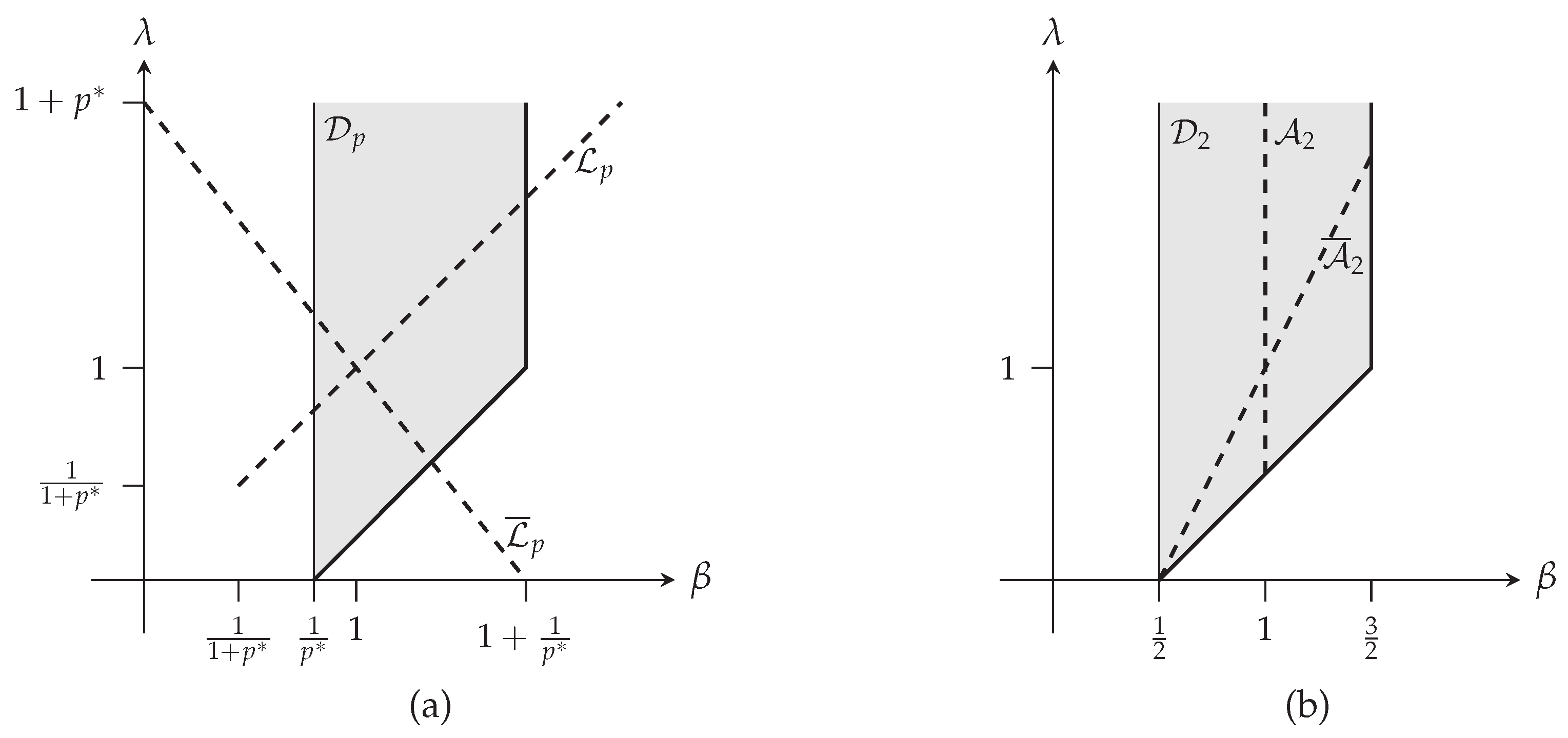
(a) the domain for a given p is represented by the gray area (here ). The thick line belongs to . The dashed line represents , corresponding to the Lutwak situation of Section 2.3.1, where the relation holds and the minimizers are explicitly known (stretched deformed Gaussian distributions), whereas corresponds to Section 2.3.2 ( and obtained by the Gagliardo–Nirenberg inequality are their restrictions to ); (b) same situation for , with the domains and (dashed lines) that correspond to the situations of Section 2.3.3 and Section 2.3.4, respectively, ( and are not represented for the clarity of the figure).
Figure 1.
(a) the domain for a given p is represented by the gray area (here ). The thick line belongs to . The dashed line represents , corresponding to the Lutwak situation of Section 2.3.1, where the relation holds and the minimizers are explicitly known (stretched deformed Gaussian distributions), whereas corresponds to Section 2.3.2 ( and obtained by the Gagliardo–Nirenberg inequality are their restrictions to ); (b) same situation for , with the domains and (dashed lines) that correspond to the situations of Section 2.3.3 and Section 2.3.4, respectively, ( and are not represented for the clarity of the figure).

Figure 2.
Given a p, the domain in gray represents , where we know that the -Fisher–Rényi complexity is optimally lower bounded and where the minimizers can be deduced from proposition 2. (a) the domain in dark gray represents , which is obviously included in ; the dot is a particular point and the dotted line represents its transform by ; (b) the domain in dark gray represents , which obviously contains represented by the dashed line; (c) same as (b) with and . This illustrates that .

Figure 3.
Fisher information (left graph), Rényi entropy power (center graph), and -Fisher–Rényi complexity (right graph) of the radial hydrogenic distribution in position space with dimensions versus the quantum numbers n and l. The complexity parameters are .
Figure 3.
Fisher information (left graph), Rényi entropy power (center graph), and -Fisher–Rényi complexity (right graph) of the radial hydrogenic distribution in position space with dimensions versus the quantum numbers n and l. The complexity parameters are .

Figure 4.
-Fisher–Rényi complexity (normalized to its lower bound), , with for the radial hydrogenic distribution in the position space with dimensions and .
Figure 4.
-Fisher–Rényi complexity (normalized to its lower bound), , with for the radial hydrogenic distribution in the position space with dimensions and .

Figure 5.
Fisher information (left graph), Rényi entropy power (center graph), and -Fisher–Rényi complexity (right graph) of the radial hydrogenic distribution in momentum space with dimensions versus the quantum numbers n and l. The complexity parameters are .
Figure 5.
Fisher information (left graph), Rényi entropy power (center graph), and -Fisher–Rényi complexity (right graph) of the radial hydrogenic distribution in momentum space with dimensions versus the quantum numbers n and l. The complexity parameters are .
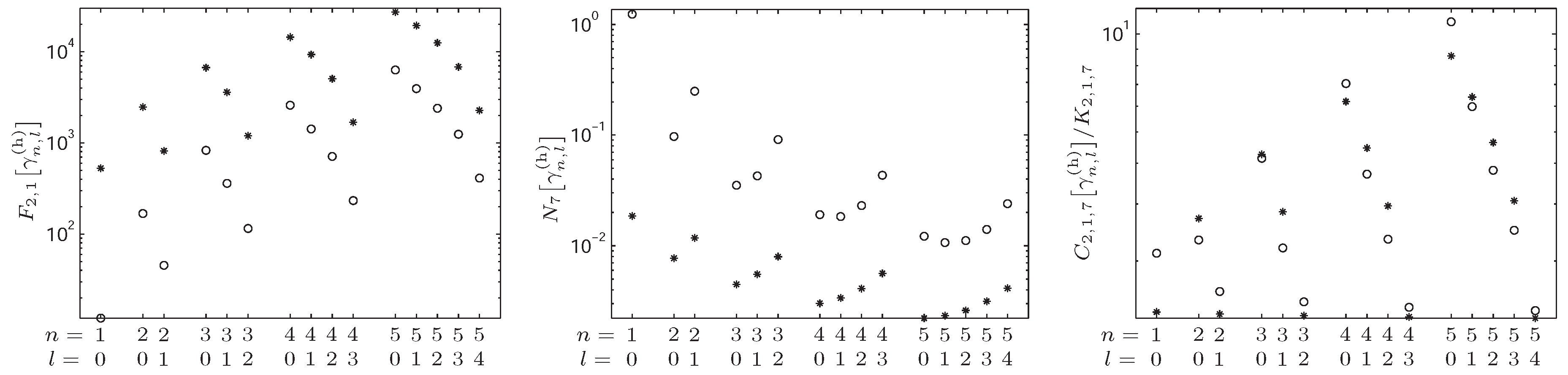
Figure 6.
-Fisher–Rényi complexity (normalized to its lower bound), , with for the radial hydrogenic distribution in the momentum space with dimensions and .
Figure 6.
-Fisher–Rényi complexity (normalized to its lower bound), , with for the radial hydrogenic distribution in the momentum space with dimensions and .
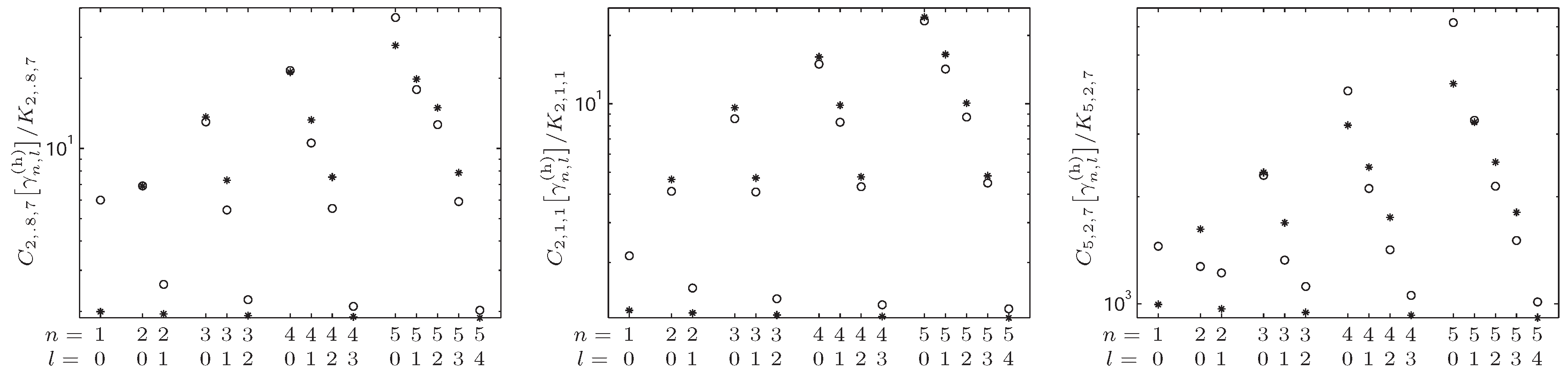
Figure 7.
Fisher information (left graph), Rényi entropy power (center graph), and -Fisher–Rényi complexity (right graph) versus n and l for the radial harmonic system in position space with dimensions . The informational parameters are .
Figure 7.
Fisher information (left graph), Rényi entropy power (center graph), and -Fisher–Rényi complexity (right graph) versus n and l for the radial harmonic system in position space with dimensions . The informational parameters are .
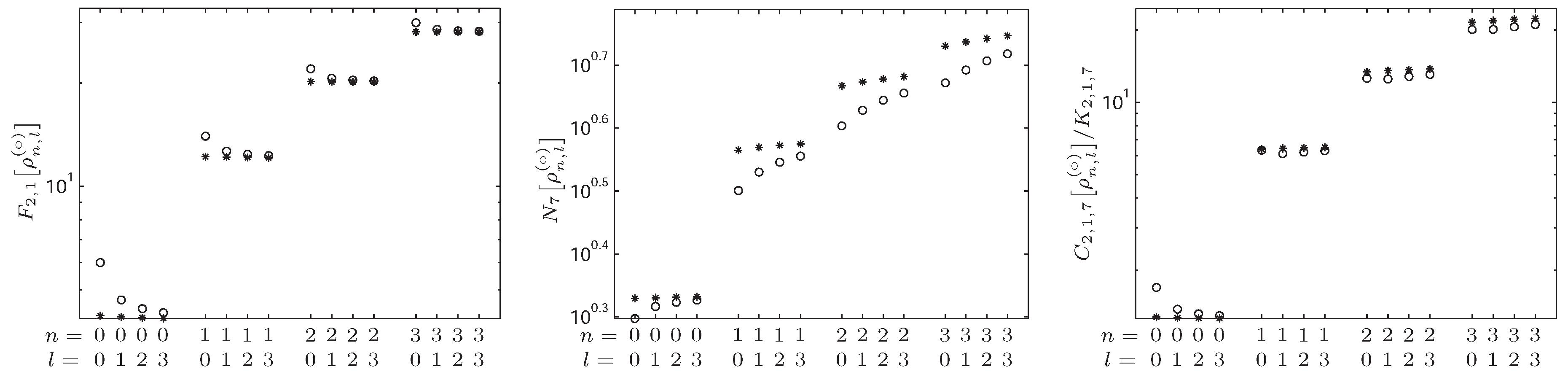
Figure 8.
-Fisher–Rényi complexity (normalized to its lower bound) with for the oscillator system in the position space with dimensions .
Figure 8.
-Fisher–Rényi complexity (normalized to its lower bound) with for the oscillator system in the position space with dimensions .
© 2017 by the authors. Licensee MDPI, Basel, Switzerland. This article is an open access article distributed under the terms and conditions of the Creative Commons Attribution (CC BY) license (http://creativecommons.org/licenses/by/4.0/).
Share and Cite
MDPI and ACS Style
Zozor, S.; Puertas-Centeno, D.; Dehesa, J.S. On Generalized Stam Inequalities and Fisher–Rényi Complexity Measures. Entropy 2017, 19, 493. https://doi.org/10.3390/e19090493
AMA Style
Zozor S, Puertas-Centeno D, Dehesa JS. On Generalized Stam Inequalities and Fisher–Rényi Complexity Measures. Entropy. 2017; 19(9):493. https://doi.org/10.3390/e19090493
Chicago/Turabian StyleZozor, Steeve, David Puertas-Centeno, and Jesús S. Dehesa. 2017. "On Generalized Stam Inequalities and Fisher–Rényi Complexity Measures" Entropy 19, no. 9: 493. https://doi.org/10.3390/e19090493
Note that from the first issue of 2016, this journal uses article numbers instead of page numbers. See further details here.