Log Likelihood Spectral Distance, Entropy Rate Power, and Mutual Information with Applications to Speech Coding


Department of Electrical and Computer Engineering, University of California, Santa Barbara, CA 93106, USA
*
Author to whom correspondence should be addressed.
Entropy 2017, 19(9), 496; https://doi.org/10.3390/e19090496
Submission received: 22 August 2017
/
Revised: 9 September 2017
/
Accepted: 10 September 2017
/
Published: 14 September 2017
(This article belongs to the Special Issue Entropy in Signal Analysis)
Abstract
:We provide a new derivation of the log likelihood spectral distance measure for signal processing using the logarithm of the ratio of entropy rate powers. Using this interpretation, we show that the log likelihood ratio is equivalent to the difference of two differential entropies, and further that it can be written as the difference of two mutual informations. These latter two expressions allow the analysis of signals via the log likelihood ratio to be extended beyond spectral matching to the study of their statistical quantities of differential entropy and mutual information. Examples from speech coding are presented to illustrate the utility of these new results. These new expressions allow the log likelihood ratio to be of interest in applications beyond those of just spectral matching for speech.
1. Introduction
We provide new expressions relating the log likelihood ratio from signal processing, the minimum mean squared prediction error from time series analysis, and the entropy power from information theory. We then show how these new expressions for the log likelihood ratio invite new analyses and insights into problems in digital signal processing. To demonstrate their utility, we present applications to speech coding and show how the entropy power can explain results that previously escaped interpretation.
The linear prediction model plays a major role in many digital signal processing applications, but none perhaps more important than linear prediction modeling of speech signals. Itakura introduced the log likelihood ratio as a distance measure for speech recognition [1], and it was quickly applied to evaluating the spectral match in other speech-processing problems [2,3,4,5]. In time series analysis, the linear prediction model, called the autoregressive (AR) model, has also received considerable attention, with a host of results on fitting AR models, AR model prediction performance, and decision-making using time series analysis based on AR models. The particular results of interest here from time series analysis are the expression for the mean squared prediction error and the decomposition in terms of nondeterministic and deterministic processes [6,7,8].
The quantity called entropy power was defined by Shannon [9], and has primarily been used in bounding channel capacity and rate distortion functions. Within the context of information theory and rate distortion theory, Kolmogorov [10] and Pinsker [11] derived an expression for the entropy power in terms of the power spectral density of a stationary random process. Interestingly, their expression for the entropy power is the same as the expression from time series analysis for the minimum mean squared prediction error. This fact was recognized by Gish and Berger in 1967, but the connection has never been formalized and exploited [12,13].
In this paper, we use the expression for the minimum mean squared prediction error to show that the log likelihood ratio equals the logarithm of the ratio of entropy powers, and then develop an expression for the log likelihood ratio in terms of the difference of differential entropies and the difference of two mutual informations. We specifically consider applications of linear prediction to speech coding, including codec performance analysis and speech codec design.
In Section 2, we define and discuss expressions for the log likelihood ratio, and in Section 3, we define and explain the entropy power and its implications in information theory. Section 4 examines the mean squared prediction error from time series analysis and relates it to entropy power. The quantities of entropy power and mean squared prediction error are then used in Section 5 to develop the new expressions for the log likelihood ratio in terms of differential entropy and mutual information. Experimental results are presented in Section 6 for several speech coding applications, and in Section 7, a detailed discussion of the experimental results is provided, as the difference in differential entropies and mutual informations reveals new insights into codec performance evaluation and codec design. Section 8 provides the experimental lessons learned and suggestions for additional applications.
2. Log Likelihood Spectral Distance Measure
A key problem in signal processing, starting in the 1970s, has been to determine an expression for the difference between the spectra of two different discrete time signals. One distance measure that was proposed by Itakura [1] and found to be effective for some speech recognition applications and for comparing the linear prediction coefficients calculated from two different signals is the log likelihood ratio defined by [2,3,4,5]:
where and are the augmented linear prediction coefficient vectors of the original signal, , and processed signal, , respectively, and V is the Toeplitz autocorrelation matrix [14,15] of the processed signal, with diagonal components N is the number of samples used for the analysis window, and n is the predictor order [5]. We thus see that is the minimum mean squared prediction error for predicting the processed signal, and that is the mean squared prediction error obtained when predicting the processed signal with the coefficients calculated based on the original signal [2,3,4,5,14,15]. Magill [2] employed the ratio to determine when to transmit linear prediction coefficients in a variable rate speech coder based on Linear Predictive Coding (LPC).
A filtering interpretation corresponding to and is also instructive [3,5]. Defining and , we consider as the mean squared prediction error when passing the signal through , which, upon letting , can be expressed as ; also, is the mean squared prediction error when passing the signal through , which can be expressed as . Here, denotes the discrete time Fourier transform of the sequence . We can thus write the log likelihood ratio in (1) in terms of the spectral densities of autoregressive (AR) processes as [3,5]:
where the spectral density divides out.
The quantity has been compared to different thresholds in order to classify how good of a spectral match is being obtained, particularly for speech signals. Two thresholds often quoted in the literature are d = 0.3, called the statistically significant threshold, and what has been called a perceptually significant threshold, d = 0.9. The value d > 0.3 indicates that “there is less than a 2% chance” that the set of coefficients are from an unprocessed signal with coefficients , and thus d = 0.3 is called the statistically significant threshold [4]. Itakura [1,4] found that for the difference in coefficients to be significant for speech recognition applications, the threshold should be 3 times the statistically significant threshold or d > 0.9. These values were based on somewhat limited experiments, and it has been noted that these specific threshold values are not set in stone, but it was generally accepted that d > 0.9 is a poor spectral fit [3,4]. Therefore, for speech coding applications, d > 0.9, is considered an indicator that the codec being evaluated is performing poorly.
The challenge with the log likelihood ratio has always been that the interpretation of the value of d when it is less than the perceptually significant threshold and greater than 0.3 is not evident. In the range 0.3 < d < 0.9, the log likelihood was simply interpreted to be an indicator that the spectral match was less than perfect, but perhaps acceptable perceptually. It appears that the lack of clarity as to the perceptual meaning of the possible values taken on by d caused it to lose favor as a useful indicator of performance in various applications.
In the sections that follow, we introduce two new additional expressions for d that allow us to better interpret the log likelihood ratio when it is less than the perceptually significant threshold of 0.9. These new interpretations admit a new modeling analysis that we show relates directly to speech codec design.
3. Entropy Power/Entropy Rate Power
For a continuous valued random variable X with probability density function p(x), we can write the differential entropy
where X has the variance . In his original paper, Shannon [9] defined what he called the derived quantity of entropy power corresponding to the differential entropy of the random variable X. In particular, Shannon defined the entropy power as the power in a Gaussian random variable having the same entropy as the given random variable X. Specifically, since a Gaussian random variable has the differential entropy, solving for and letting we have that the corresponding entropy power is
where here h(X) is not Gaussian, but it is the differential entropy of the “original” random variable.
Generally, we will be modeling our signals of interest as stationary random processes. If we let X be a stationary continuous-valued random process with samples , then the differential entropy rate of the process X is [16]
We assume that this limit exists in our developments and we drop the overbar notation and use as before . Thus, for random processes, we use the entropy rate in the definition of entropy power, which yields the nomenclature entropy rate power.
We now consider a discrete-time stationary random process X with correlation function and define its periodic discrete-time power spectral density for For an n-dimensional random process with correlation matrix , we know that the determinant of is the product of its eigenvalues, so , and we can write
To obtain an expression for the entropy rate power, we note that the differential entropy of a Gaussian random process with the given power spectral density, , and correlation matrix is , then solving for and taking the limit as in (7), we can write the entropy rate power Q as [8,9]
One of the primary applications of Q has been for developing a lower bound to the rate distortion function [9,12,13]. Note that, in defining Q, we have not assumed that the original random process is Gaussian. The Gaussian assumption is only used in Shannon’s definition of entropy rate power. In this paper, we expand the utility of entropy rate power to digital signal processing, and in particular, in our examples, to speech codec performance evaluation and codec design.
4. Mean Squared Prediction Error
To make the desired connection of entropy rate power with the log likelihood ratio, we now develop some well-known results in statistical time series analysis. As before, we start with a discrete-time stationary random process X with autocorrelation function and corresponding power spectral density , again without the Gaussian assumption. It can be shown that the minimum mean squared prediction error (MMSPE) for the one-step ahead prediction of , given all can be written as [6,8]
which, as was first observed by Gish and Berger, is the same expression as for the entropy rate power Q of the signal [13].
The entropy rate power is defined by Shannon to be the power in a Gaussian signal with the same differential entropy as the original signal. The signal being analyzed is not assumed to be Gaussian, but to determine the entropy rate power, Q, we use the signal differential entropy, whatever distribution and differential entropy it has, in the relation for a Gaussian process. It is tempting to conclude that, given the MMSPE of a signal, we can use the entropy rate power connection to the differential entropy of a Gaussian process to explicitly exhibit the differential entropy of the signal being analyzed as ; however, this is not true and this conclusion only follows if the underlying signal being analyzed is Gaussian.
Explicitly, Shannon’s definition of entropy rate power is not reversible. Shannon stated clearly that entropy rate power is a derived quantity [9]. For a known differential entropy, we can calculate the entropy rate power as in Shannon’s original expression. If we start with the MMSPE or a signal variance, we cannot obtain the true differential entropy from the Gaussian expression as above. Given an MMSPE, however, what we do know is that there exists a corresponding differential entropy and we can use the MMSPE to define an entropy rate power in terms of the differential entropy of the original signal. We just cannot calculate the differential entropy using the Gaussian expression.
While the expression for the MMSPE is well-known in digital signal processing, it is the connection to the entropy rate power Q and thus to the differential entropy of the signal, which has not been exploited in digital signal processing, that opens up new avenues for digital signal processing and for interpreting past results. Specifically, we can interpret comparisons of MMSPE as comparisons of entropy powers, and thus interpret these comparisons in terms of the differential entropies of the two signals. This observation provides new insights into a host of signal processing results that we develop in the remainder of the paper.
5. Connection to the Log Likelihood Ratio
To connect the entropy rate power to the log likelihood ratio, we focus on autoregressive processes or the linear prediction model, which is widely used in speech processing and speech coding. We recognize as the when predicting a processed or coded signal with the linear prediction coefficients optimized for that signal, and we also see that is the MSPE, not the minimum, when predicting the processed signal with the coefficients optimized for the original unprocessed signal. The interpretation of as an entropy rate power is direct, since we know that, for a random variable X with zero mean and variance the Gaussian distribution lower bounds its differential entropy, so , and thus it follows by definition that Therefore, , since here.
However, is not the minimum MSPE for the process being predicted, because the prediction coefficients were calculated on the unprocessed signal but used to predict the processed signal, so it does not automatically achieve any lower bound. What we do is define as the of a new process, so that for this new process, we can obtain a corresponding entropy rate power as This is equivalent to associating the suboptimal prediction error with a whitened nondeterministic component [6,8]. In effect, the resulting is the maximum power in the nondeterministic component that can be associated with .
Using the expression for entropy power Q from Equation (4), substituting for both and , and taking the logarithm of the two expressions, we have that
where is the differential entropy of the signal generated by passing the processed signal through a linear prediction filter using the linear prediction coefficients computed from the unprocessed signal, and is the differential entropy of the signal generated by passing the processed signal through a linear filter using the linear coefficients calculated from the processed signal. Gray and Markel [3] have used such linear filter analogies for the log likelihood ratio in terms of a test signal and a reference signal before for spectral matching studies, and other log likelihood ratios can be investigated based on switching the definitions of the test and reference.
It is now evident that the log likelihood ratio has an interpretation beyond the usual viewpoint of just involving a ratio of prediction errors or just as a measure of a spectral match. We now see that the log likelihood ratio is interpretable as the difference between two differential entropies, and although we do not know the form or the value of each differential entropy, we do know their difference.
We can provide an even more intuitive form of the log likelihood ratio: since we have as the MMSPE when predicting the processed signal with the linear prediction coefficients optimized for that signal, and we have that is the MMSPE when predicting the processed signal with the coefficients optimized for the original unprocessed signal, we can add and subtract , the differential entropy of the processed signal, to Equation (10) to obtain
where, as before, we have used the notation for the predictor, obtaining and for the predictor, and generating This is particularly meaningful, since it indicates the difference in the mutual information between the processed signal and the predicted signal based on coefficients optimized for the processed signal, and the mutual information between the processed signal and the predicted signal based on using the processed signal and the coefficients optimized for the unprocessed signal. Mutual information is always greater than or equal to zero, so since we would expect that , this result is intuitively very satisfying. We emphasize that we do not know the individual mutual informations but we do know their difference.
In the case of any speech processing application, we see that the log likelihood ratio is now not only interpretable in terms of a spectral match, but also in terms of matching differential entropies or the difference between mutual informations. As we shall demonstrate, important new insights are now available.
6. Experimental Results
To examine the new insights provided by the new expressions for the log likelihood ratio, we study the log likelihood ratio for three important speech codecs that have been used extensively in the past, namely G.726 [17], G.729 [18], and AMR-NB [19], at different transmitted bit rates. Note that we do not study the newest standardized voice codec, designated Enhanced Voice Services (EVS) [20], since it is not widely deployed at present. Further, AMR was standardized in December 2000 and has been the default codec in 3GPP cellular systems, including Long Term Evolution (LTE), through 2014, when the new EVS codec was standardized [19,21]. LTE will still be widely used until there is a larger installed base of the EVS codec. AMR is also the codec (more specifically, its wideband version) that is planned for use in U.S. next generation emergency first responder communication systems [22]. For more information on these codecs, the speech coding techniques, and the cellular applications, see Gibson [23].
We use two different speech sequences as inputs, “We were away a year ago”, spoken by a male speaker, and “A lathe is a big tool”, spoken by a female speaker, filtered to 200 to 3400 Hz, often called narrowband speech, and sampled at 8000 samples/s. In addition to calculating the log likelihood ratio, we also use the Perceptual Evaluation of Speech Quality-Mean Opinion Score (PESQ-MOS) [24] to give a general guideline as to the speech quality obtained in each case.
After processing the original speech through each of the codecs, we employed a 25 ms Hamming window and calculated the log likelihood ratio over nonoverlapping 25 ms segments. Studies of the effect of overlapping the windows by 5 ms and 10 ms showed that the results and conclusions remain the same as for the nonoverlapping case.
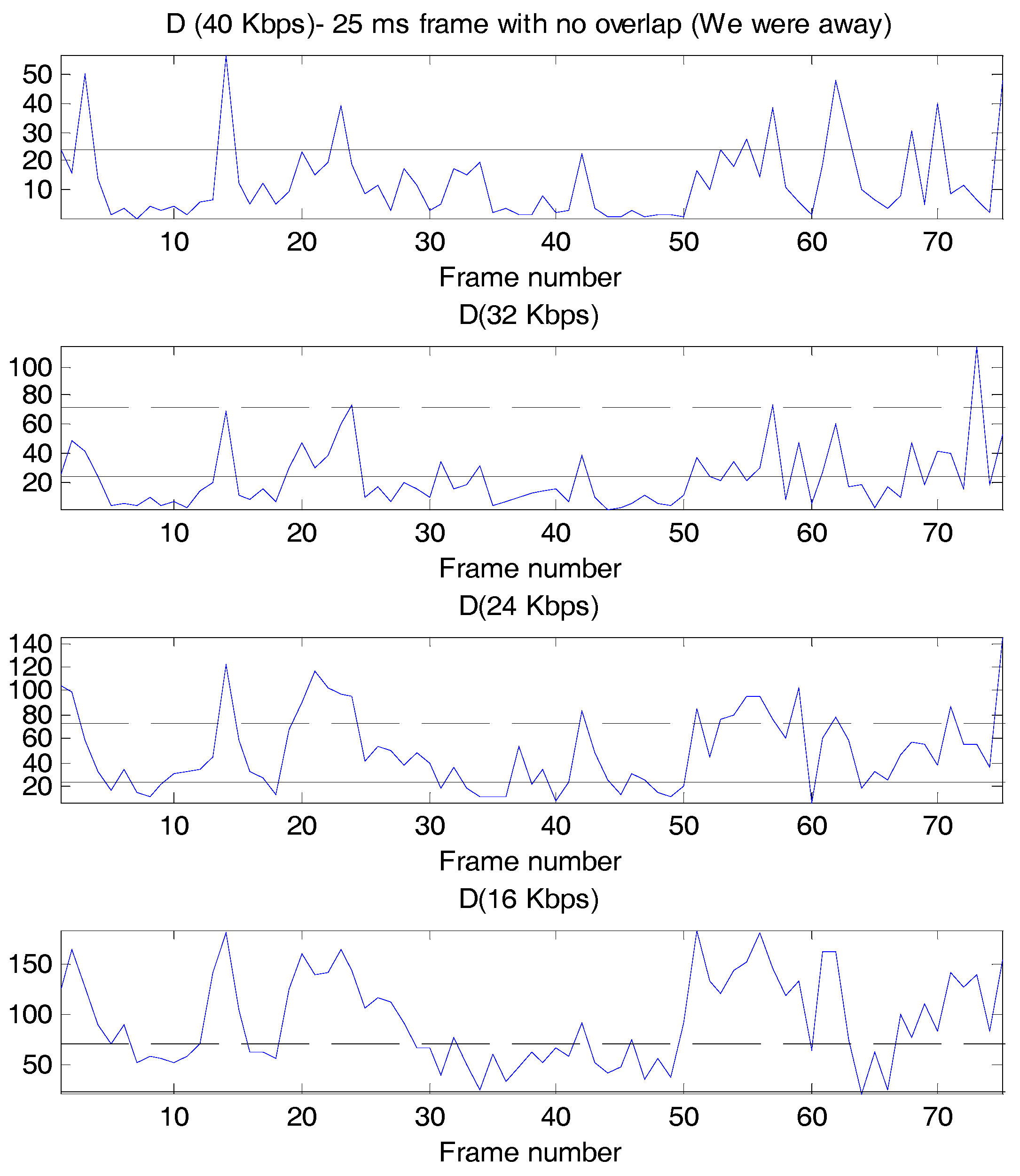
Common thresholds designated in past studies for the log likelihood ratio, d, are what is called a statistically significant threshold of 0.3 and a perceptually significant threshold of 0.9. Of course, neither threshold is a precise delineation, and we show in our studies that refinements are needed. We also follow prior conventions and study a transformation of d that takes into account the effects of the chosen window [8], namely, , where is the effective window length, which for the Hamming window is where N is the rectangular window length of for 25 ms and 8000 samples/s [4]. With these values, we set the statistically significant and perceptually significant thresholds for D at 24 and 72, respectively.
6.1. G.726: Adaptive Differential Pulse Code Modulation
Adaptive differential pulse code modulation (ADPCM) is a time-domain waveform-following speech codec, and the International Standard for ADPCM is ITU-T G.726. G.726 has the four operational bit rates of 16, 24, 32, and 40 Kbps, corresponding to 2, 3, 4, and 5 bits/sample scalar quantization of a prediction residual. ADPCM is the speech coding technique that was first associated with the log likelihood ratio; so, it is an important codec to investigate initially.
Figure 1 shows the D values as a function of frame number, with the perceptually and statistically significant thresholds superimposed where possible, for the bit rates of 40, 32, 24, and 16 Kbps. Some interesting observations are possible from these plots. First, clearly the log likelihood varies substantially across frames, even at the highest bit rate of 40 Kbps. Second, even though designated as “toll quality” by ITU-T, G.726 at 32 Kbps has a few frames where the log likelihood ratio is larger than even the perceptually significant threshold. Third, as would be expected, as the bit rate is lowered, the number of frames that exceed each of the thresholds increases, and, in fact, at 16 Kbps, only the perceptually significant threshold is drawn on the figure, since the statistically significant threshold is so low in comparison. Fourth, the primary distortion heard in ADPCM is granular quantization noise, or a hissing sound, and in lowering the rate from 32 to 24 to 16 Kbps, an increase in the hissing sound is audible, and a larger fraction of the log likelihood values exceeds the perceptually significant threshold.
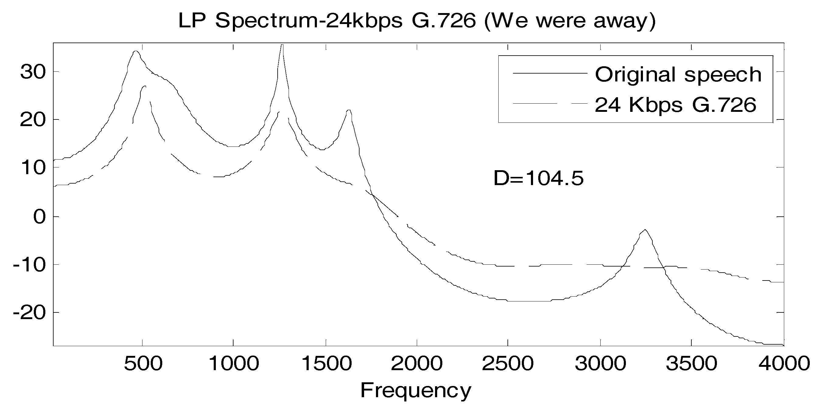
It is useful to associate a typical spectral match to a value of D, so in Figure 2, Figure 3 and Figure 4, we show the linear prediction spectra of three frames of speech coded at 24 Kbps: one frame with a D value less than the statistically significant threshold, one with a D value between the statistically significant and the perceptually significant threshold, and one with a D value greater than both thresholds. In Figure 2, D = 11, considerably below both thresholds, and visually, the spectral match appears to be good. In Figure 3, we have D = 36.5 > 24, and the spectral match is not good at all at high frequencies, with two peaks, called formants, at higher frequencies, poorly reproduced. The linear prediction (LP) spectrum corresponding to a log likelihood value of D = 104.5 > 72 is shown in Figure 4, where the two highest frequency peaks are not reproduced at all in the coded speech, and the spectral shape is not well approximated either. Figure 2 and Figure 4 would seem to validate, for these particular cases, the interpretation of D = 24 and D = 72 as statistically and perceptually significant thresholds, respectively, for the log likelihood ratio. The quality of the spectral match in Figure 3 would appear to be unsatisfactory and so the statistically significant threshold is also somewhat validated; however, it would be useful if something more interpretive or carrying more of a physical implication could be concluded for this D value.
Motivated by the variation in the values of the log likelihood ratio across frames, we calculate the percentage of frames that fall below the statistically significant threshold, in between the statistically significant and perceptually significant thresholds, and above the perceptually significant threshold for each G.726 bit rate for the sentence “We were away a year ago” and for the sentence “A lathe is a big tool”, and list these values in Table 1 and Table 2, respectively, along with the corresponding signal-to-noise ratios in dB and the PESQ-MOS values [23].
A few observations are possible from the data in Table 1 and Table 2. From Table 1, we see that for 24 Kbps, the PESQ-MOS indicates a noticeable loss in perceptual performance, even though the log likelihood ratio has values above the perceptually significant threshold only 25% of the time. Although not as substantial as in Table 1, the PESQ-MOS at 24 Kbps in Table 2 shows that there is a noticeable loss in quality even though the log likelihood ratio exceeds the perceptually significant threshold only 9% of the time. However, it is notable that at 24 Kbps in Table 1, D > 24 for 75% of the frames, and in Table 2, for more than 50% of the frames. This leads to the needed interpretation of the log likelihood ratio as a comparison of distributional properties rather than just the logarithm of the ratio of mean squared prediction errors (MSPEs) or as a measure of spectral match.
Considering the log likelihood as a difference between differential entropies, we can conclude that the differential entropy of the coded signal when passed through a linear prediction filter based on the coefficients computed on the original speech is substantially different from the differential entropy when passing the coded signal through a linear prediction filter based on the coefficients calculated on the coded speech signal. Further, in terms of the difference between two mutual informations, the mutual information between the coded speech signal and the signal passed through a linear filter with coefficients calculated based on the coded speech is substantially greater than the mutual information between the coded speech and the coded speech passed through a linear prediction filter with coefficients calculated on the original speech.
Notice also that, for both the differential entropy and the mutual information interpretations, as the coded speech signal approaches that of the original signal, that is, as the rate for G.726 is increased or the quantizer step size is reduced, the difference in differential entropies and the difference in mutual informations each approach zero.
6.2. G.729
We also study the behavior of the log likelihood ratio for the ITU-T standardized codec G.729 at 8 Kbps. Even though G.729 is not widely used at this point, we examine its performance because of its historical importance as the forerunner of today’s best codecs, and also so that we can compare AMR-NB at 7.95 Kbps to G.729 at 8 Kbps, both of which fall into the category of code-excited linear prediction (CELP) approaches [23].
Table 3 and Table 4 show the percentage of frames in the various D ranges along with the PESQ-MOS value for the two sentences “We were away a year ago” and “A lathe is a big tool”. SNR is not included, since it is not a meaningful performance indicator of CELP codecs.
As expected, the PESQ-MOS values are near 4.0 in both cases and in neither table does any fraction of D exceed the perceptually significant threshold. Strikingly, however, in both tables, more than 50% of the frames have a D value above the statistically significant threshold. To think about this further, we note the bit allocation for the G.729 codec is, for each 20 ms interval, 36 bits for the linear prediction model, 28 bits for the pitch delay, 28 bits for the codebook gains, and 68 bits for the fixed codebook excitation. One fact that stands out is that the parameters for the linear prediction coefficients are allocated 36 bits when 24 bits/20 ms frame is considered adequate [25]. In other words, the spectral match should be quite good for most of the frames, and yet, based on D, more than 50% of the frames imply a less than high quality spectral match over the two sentences.
Further analysis of this observation is possible in conjunction with the AMR-NB results.
6.3. AMR-NB
The adaptive multirate (AMR) set of codecs is a widely installed, popular speech codec used in digital cellular and Voice over Internet Protocol (VoIP) applications [22,26]. A wideband version (50 Hz to 7 kHz input bandwidth) is standardized, but a narrowband version is also included. The AMR-NB codec has rates of 12.2, 10.2, 7.95, 7.4, 6.7, 5.9, 5.15, and 4.75 Kbps.
In Table 5 and Table 6, we list the percentage of frames with the log likelihood ratio in several ranges for all of the AMR-NB bit rates and the two sentences “We were away a year ago” and “A lathe is a big tool”, respectively. At a glance, it is seen that although the PESQ-MOS changes by over 0.5 for the sentence “We were away a year ago” and by more than 0.8 for the sentence “A lathe is a big tool” as the rates decrease, there are no frames above the perceptually significant threshold! This observation points out that the “perceptually significant” threshold is fairly arbitrary, and also that the data need further analysis.
A more subtle observation is that, for the sentence “We were away a year ago”, changes in PESQ-MOS of more than 0.1 align with a significant increase in the percentage of frames satisfying . The converse can be stated for the sentence “A lathe is a big tool”, namely that when the percentage of frames satisfying increases substantially, there is a change in PESQ-MOS of 0.1 or more. There are two changes in PESQ-MOS of about 0.1 for this sentence, which correspond to only slight increases in the number of frames greater than the statistically significant threshold.
Analyses of the number of bits allocated to the different codec parameters allow further important interpretations of D, particularly in terms of the new expressions involving differential entropy and mutual information. Table 7 shows the bits/20 ms frame for each AMR-NB bit rate for each of the major codec parameter categories, predictor coefficients, pitch delay, fixed codebook, and codebook gains. Without discussing the AMR-NB codec, we point out in summary that, first, the AMR-NB codec does not quantize and code the predictor coefficients directly, but quantizes and codes a one-to-one transformation of these parameters called line spectrum pairs [15,23], but we use the label “predictor coefficients”, since these are the model parameters discussed in this paper.
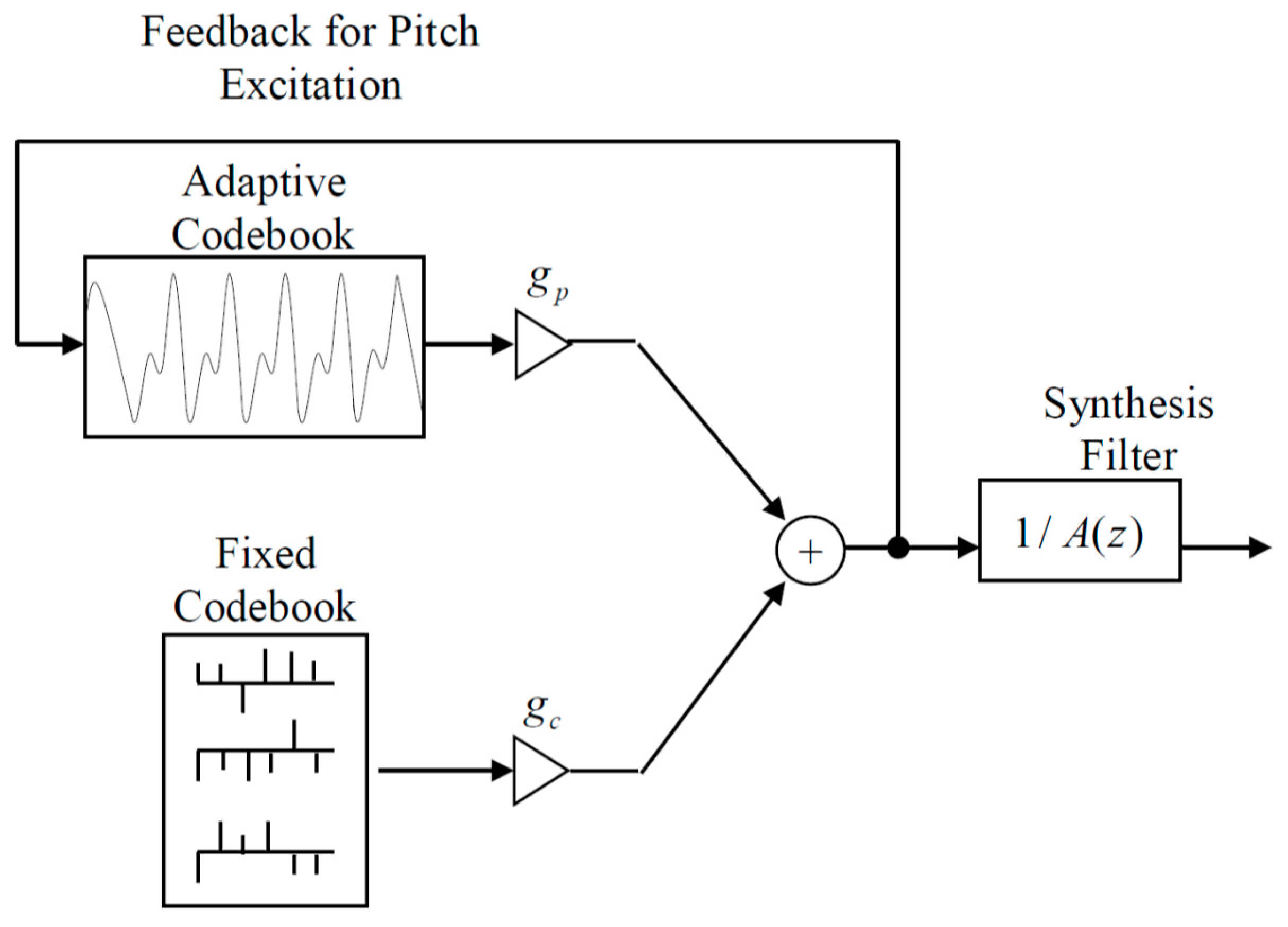
Further, as shown in Figure 5, the synthesizers or decoders in these speech codecs (as well as G.729) are linear prediction filters with two excitations added together, the adaptive codebook, depending on the pitch delay, and the fixed codebook, which is intended to capture the elements of the residual error that are not predictable using the predictor coefficients and the long-term pitch predictor.
Reading across the first row of Table 7, we see that the number of bits allocated to the predictor coefficients, which model the linear prediction spectra, is almost constant for the bit rates of 10.2 down to 5.9 Kbps. Referring now to Table 5 and Table 6, we see that for the rates 7.95 down through 5.9 kbps, the PESQ-MOS with the percentage of frames greater than the statistically significant threshold but less than the perceptually significant threshold is roughly constant as well. The outlier for the rates with the same number of bits allocated to predictor coefficients in terms of a lower percentage D value above the statistically significant threshold is 10.2 Kbps. What is different about this rate? From Table 7, we see that the fixed codebook has a much finer representation of the prediction residual, since it is allocated 124 bits/frame at 10.2 Kbps compared to only 68 or fewer bits for the other lower rates. Focusing on the fixed codebook bit allocation, we see that both the 7.95 and 7.4 Kbps rates have 68 bits assigned to this parameter, and the PESQ-MOS and the percentage of frames satisfying are almost identical, the latter of which is much higher than 10.2 Kbps, for these two rates.
We further see that the continued decrease in PESQ-MOS for “A lathe is a big tool” in Table 6 as the rate is reduced from 7.4 to 6.7 to 5.9 to 5.15 corresponds to decreases for the fixed codebook bit allocation. This same trend is not observed in Table 5. The reason for this appears to be that the sentence “We were away a year ago” is almost all what is called Voiced speech, which is well-modeled by linear prediction [23], and the bits allocated for the predictor coefficients remain almost constant over those rates. However, the sentence “A lathe is a big tool” has considerable Unvoiced speech content, which has more of a noise-like spectrum not captured well by a linear prediction model. As a result, the fixed codebook excitation is more important for this sentence.
We put all of these analyses in the context of the new interpretations of the log likelihood ratio in the next section.
7. Modeling, Differential Entropy, and Mutual Information
For linear prediction speech modeling, there is a tradeoff between the number of bits and the accuracy of the representation of the predictor coefficients as opposed to the number of bits allocated to the linear prediction filter excitation. For a purely AR process, if we know the predictor order and the predictor coefficients exactly, the MSPE will be the variance of the AR process driving term. If we now try to code this AR process using a linear prediction based codec, such as CELP, there is a tradeoff between the number of bits allocated to the predictor coefficients, which corresponds with the number and accuracy of coefficients used to approximate the AR process, and the number of bits used to model the excitation of the AR process; that is, the linear filter excitation.
Any error in the number and accuracy of the predictor or AR process coefficients is translated into a prediction error that must be modeled by the excitation, thus requiring more bits to be allocated to the codebook excitation. Also, if we use a linear prediction-based codec on a segment that is not well-modeled by an AR process, the prediction will be poor and the number of bits required for the excitation will need to increase.
While the spectral matching interpretation of the log likelihood ratio captures the error in the fit of the order and accuracy of the predictor for the predictor part, it is not as revelatory for the excitation. For the excitation, the expression for d in terms of differential entropies illuminates the change in randomness caused by the accuracy of the linear prediction. For example, the change in the percentage of d values that fall within in Table 5 when the rate is decreased from 10.2 to 7.95 or 7.4 is not explained by the predictor fit, since the number of bits allocated to the coefficients is not decreased. However, this change is quite well-indicated by the change in bits allocated to the fixed codebook excitation. The difference in the two differential entropies is much better viewed as the source of the increase than the spectral fit.
As discussed earlier, the interaction between the spectral fit and the excitation is illustrated in Table 6 when the rate is changed from 6.7 to 5.9, the number of bits allocated to the predictor is unchanged but the fixed codebook bits are reduced, and this produces only a slight change in the percentage of d values that fall within and a 0.1 decrease in PESQ-MOS. Further, changing the rate from 5.9 to 5.15, both the number of bits allocated to the predictor and to the fixed codebook are both reduced, and there is a large jump in the percentage of d values that fall within and a 0.12 decrease in PESQ-MOS. A decrease in bits for spectral modeling without increasing the bits allocated to the codebook causes the predictor error to grow, which is again better explained by the difference in differential entropy interpretation of d.
Similarly, the expression for d as a difference in mutual informations illuminates the source of the errors in the approximation more clearly than just a spectral match, since mutual information captures distributional differences beyond correlation. For example, G.729 has more bits allocated to the predictor coefficients than AMR-NB at 10.2 Kbps, yet in Table 3 and Table 4 for G.729, we see a much larger percentage of d values that fall within . This indicates other, more subtle modeling mismatches that suit the mutual information or differential entropy interpretations of d.
Certainly, with these new interpretations, d is a much more useful quantity for codec design beyond the expression for spectral mismatch. Much more detailed analyses of current codecs using this new tool are indicated, and d should find a much larger role in the design of future speech codecs.
8. Finer Categorization and Future Research
In hindsight, it seems evident, from the difference in the differential entropies expression and the difference in the mutual information expressions, that to utilize d as an effective tool in digital signal analysis, a finer categorization of d beyond just greater than 0.3, between 0.3 and 0.9, and greater than 0.9, would be much more revealing. For example, even though the fraction of values within an interval does not change, the number of values in the upper portion of the interval could have changed substantially. Future studies should thus incorporate a finer categorization of d in order to facilitate deeper analyses.
Even though the new interpretations of d have been quite revealing for speech coding, even more could be accomplished on this topic with a finer categorization. Additionally, the log likelihood ratio now clearly has a utility in signal analysis, in general, beyond speech, and should find applications to Electromyography (EMG), Electroencephalography (EEG), and Electrocardiogram (ECG) analyses among many other applications, where spectral mismatch alone is not of interest. In particular, the ability to use d to discover changes in differential entropy in the signals or to recognize the change in the mutual information between processed (for example, filtered or compressed) signals and unprocessed signals should prove useful.
Author Contributions
J. Gibson provided the theoretical developments, P. Mahadevan performed the speech coding experiments, and J. Gibson wrote the paper.
Conflicts of Interest
The authors declare no conflict of interest.
References
- Itakura, F. Minimum prediction residual principle applied to speech recognition. IEEE Trans. Acoust. Speech Signal Process. 1975, 23, 67–72. [Google Scholar]
- Magill, D.T. Adaptive speech compression for packet communication systems. In Proceedings of the Conference Record of the IEEE National Telecommunications Conference, Atlanta, GA, USA, 26–28 November 1973. [Google Scholar]
- Gray, A.H., Jr.; Markel, J.D. Distance measures for speech processing. IEEE Trans. Acoust. Speech Signal Process. 1976, 24, 380–391. [Google Scholar] [CrossRef]
- Sambur, M.R.; Jayant, N.S. LPC analysis/synthesis from speech inputs containing quantizing noise or additive white noise. IEEE Trans. Acoust. Speech Signal Process. 1976, 24, 488–494. [Google Scholar] [CrossRef]
- Crochiere, R.E.; Rabiner, L.R. An interpretation of the log likelihood ratio as a measure of waveform coder performance. IEEE Trans. Acoust. Speech Signal Process. 1980, 28, 318–323. [Google Scholar] [CrossRef]
- Grenander, U.; Rosenblatt, M. Statistical Analysis of Stationary Time Series; Wiley: Hoboken, NJ, USA, 1957. [Google Scholar]
- Grenander, U.; Szego, G. Toeplitz Forms and Their Applications; University of California Press: Berkeley, CA, USA, 1958. [Google Scholar]
- Koopmans, L.H. The Spectral Analysis of Time Series; Academic Press: Cambridge, MA, USA, 1974. [Google Scholar]
- Shannon, C.E. A mathematical theory of communication. Bell Syst. Tech. J. 1948, 27, 379–423. [Google Scholar]
- Kolmogorov, A.N. On the Shannon theory of information transmission in the case of continuous signals. IRE Trans. Inf. Theory 1956, 2, 102–108. [Google Scholar] [CrossRef]
- Pinsker, M.S. Information and Information Stability of Random Variables and Processes; Holden-Day: San Francisco, CA, USA, 1964. [Google Scholar]
- Berger, T. Rate Distortion Theory: A Mathematical Basis for Data Compression; Prentice-Hall: Upper Saddle River, NJ, USA, 1971. [Google Scholar]
- Berger, T.; Gibson, J.D. Lossy source coding. IEEE Trans. Inf. Theory 1998, 44, 2693–2723. [Google Scholar] [CrossRef]
- Gibson, J.D. Digital Compression for Multimedia: Principles and Standards; Morgan-Kaufmann: Burlington, MA, USA, 1998; pp. 142–147. [Google Scholar]
- Rabiner, L.R.; Schafer, R.W. Theory and Applications of Digital Speech Processing; Prentice Hall: Upper Saddle River, NJ, USA, 2011; pp. 480–483. [Google Scholar]
- El Gamal, A.; Kim, Y.-H. Network Information Theory; Cambridge University Press: Cambridge, UK, 2011. [Google Scholar]
- 40, 32, 24, 16 Kbits/s Adaptive Differential Pulse Code Modulation (ADPCM). Available online: https://www.itu.int/rec/T-REC-G.726-199012-I/en (accessed on 12 September 2017).
- Coding of Speech at 8 kb/s Using Conjugate-Structure Algebraic-Code-Excited Linear Prediction (CS-ACELP). Available online: https://www.ece.cmu.edu/~ece796/documents/g729.pdf (accessed on 12 September 2017).
- Mandatory Speech Codec Speech Processing Functions. Available online: http://www.qtc.jp/3GPP/Specs/26071-a00.pdf (accessed on 12 September 2017).
- Dietz, M.; Multrus, M.; Eksler, V.; Malenovsky, V.; Norvell, E.; Pobloth, H.; Miao, L.; Wang, Z.; Laaksonen, L.; Vasilache, A.; et al. Overview of the EVS codec architecture. In Proceedings of the IEEE International Conference on the Acoustics, Speech and Signal Processing (ICASSP), Brisbane, Australia, 19–24 April 2015; pp. 5698–5702. [Google Scholar]
- Dietz, M.; Pobloth, H.; Schnell, M.; Grill, B.; Gibbs, J.; Miao, L.; Järvinen, K.; Laaksonen, L.; Harada, N.; Naka, N.; et al. Standardization of the new 3GPP EVS codec architecture. In Proceedings of the IEEE International Conference on Acoustics, Speech and Signal Processing (ICASSP), Brisbane, Australia, 19–24 April 2015; pp. 5703–5707. [Google Scholar]
- U.S. Public Safety Research Program. Objective Speech Quality Estimates for Project 25/Voice over Long Term Evolution (P25/VoLTE) Interconnections; Technical Report, DHS-TR-PSC-13-01; Department of Homeland Security, Science and Technology Directorate: Washington DC, USA, March 2013.
- Gibson, J.D. Speech compression. Information 2016, 7, 32. [Google Scholar] [CrossRef]
- Perceptual Evaluation of Speech Quality (PESQ): An Objective Method for End-to-End Speech Quality Assessment of Narrowband Telephone Networks and Speech Codecs. Available online: http://www.itu.int/rec/T-REC-P.862-200102-I/en (accessed on 12 September 2017).
- Paliwal, K.K.; Atal, B.S. Efficient vector quantization of LPC parameters at 24 bits/frame. IEEE Trans. Speech Audio Process. 1993, 1, 3–14. [Google Scholar] [CrossRef]
- Holma, H.; Toskala, A. LTE for UMTS—OFDMA and SC-FDMA Based Radio Access; Wiley: Chichester, UK, 2009; pp. 259–281. [Google Scholar]
Figure 1.
D values for G.726 at various bit rates for “We were away a year ago”. ____: Statistically significant threshold. _ _ _: Perceptually significant threshold.
Figure 1.
D values for G.726 at various bit rates for “We were away a year ago”. ____: Statistically significant threshold. _ _ _: Perceptually significant threshold.

Figure 2.
Comparison of linear prediction (LP) spectra of original and 24 Kbps G.726 “We were away a year ago” where D = 11.
Figure 2.
Comparison of linear prediction (LP) spectra of original and 24 Kbps G.726 “We were away a year ago” where D = 11.
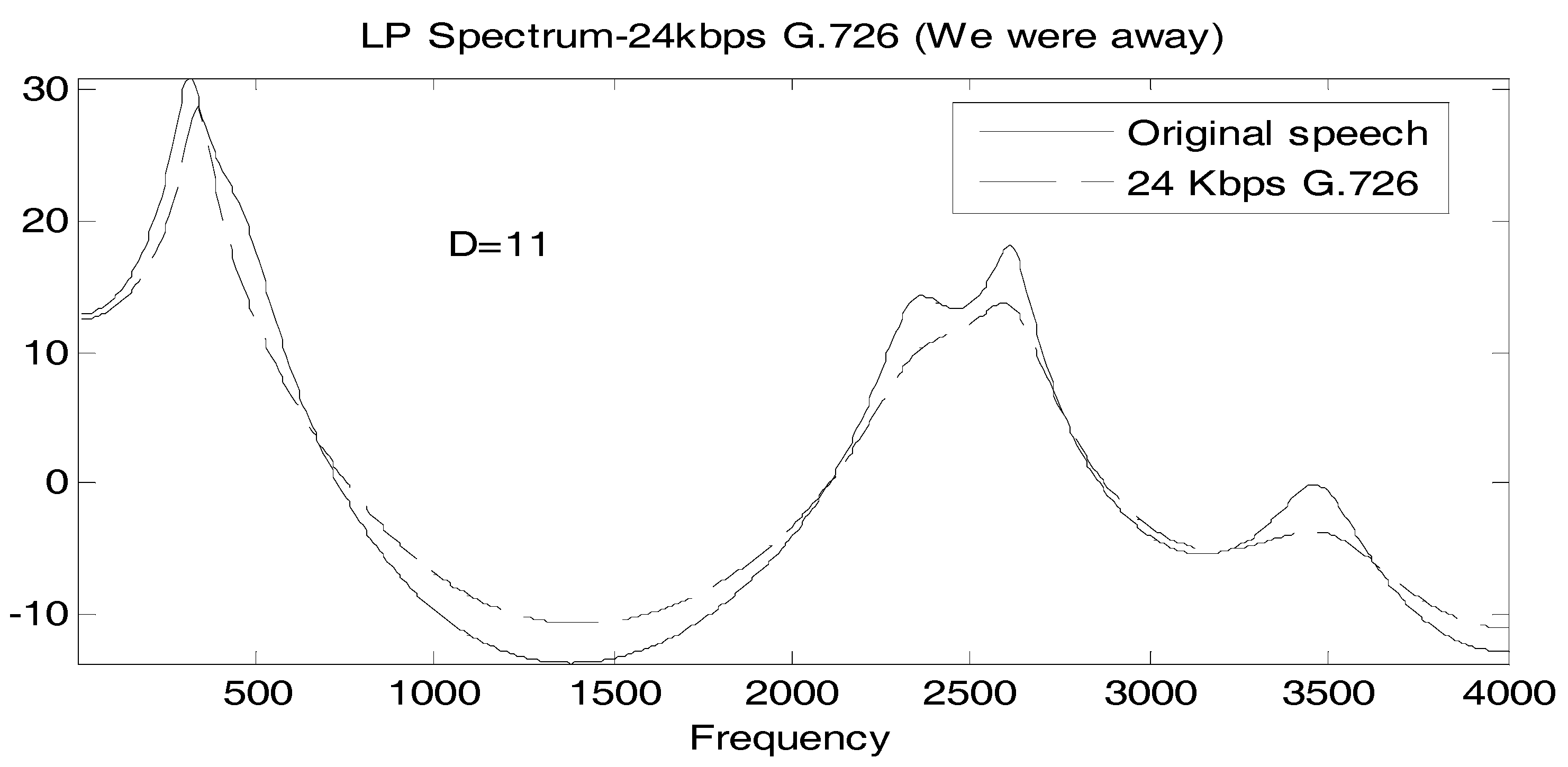
Figure 3.
Comparison of LP spectra of original and 24 Kbps G.726 “We were away a year ago” where D = 36.5.
Figure 3.
Comparison of LP spectra of original and 24 Kbps G.726 “We were away a year ago” where D = 36.5.
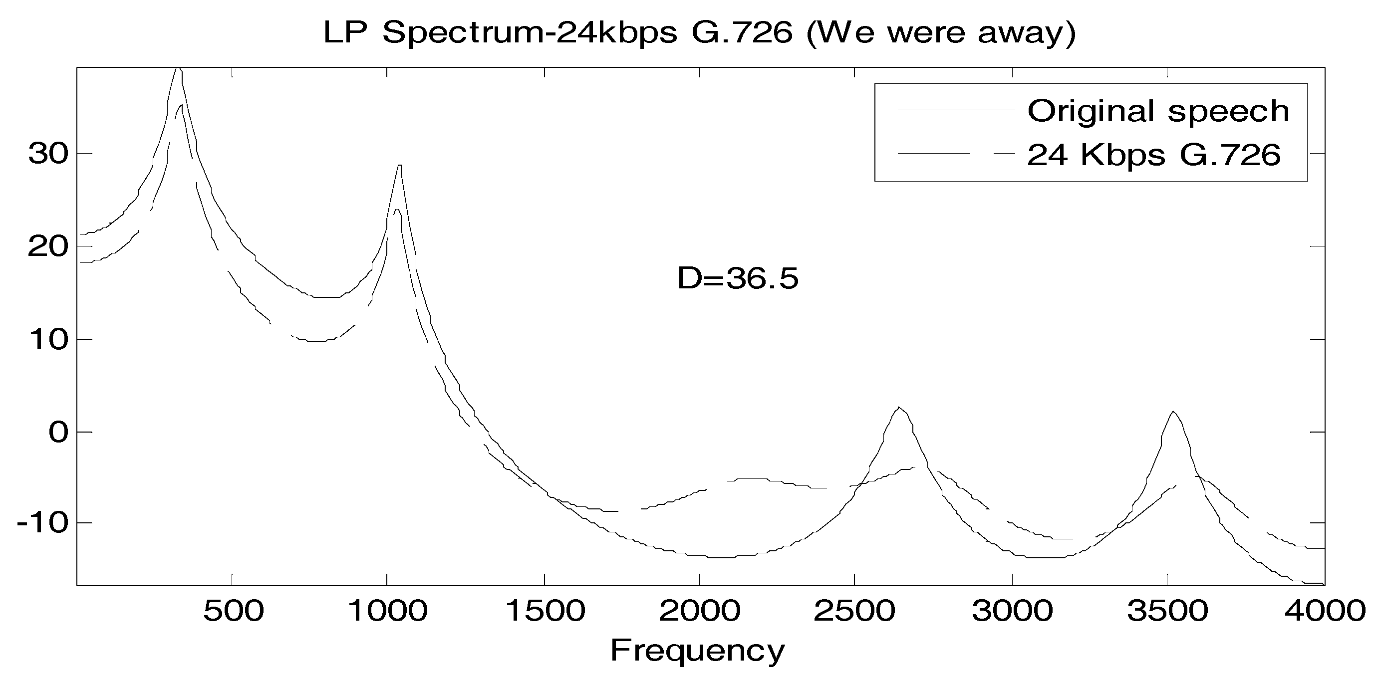
Figure 4.
Comparison of LP spectra of original and 24 Kbps G.726 “We were away a year ago” where D = 104.5.
Figure 4.
Comparison of LP spectra of original and 24 Kbps G.726 “We were away a year ago” where D = 104.5.

Figure 5.
General Block Diagram of a code-excited linear prediction (CELP) Decoder.

Table 1.
D and PESQ values for G.726 “We were away a year ago”.
| Bit Rate (Kbps) | % Frames with D < 24 | % Frames with 24 < D < 72 | % Frames with D > 72 | PESQ-MOS | SNR (dB) |
|---|---|---|---|---|---|
| 40 | 85.83 | 14.67 | 0 | 4.163 | 24.3077 |
| 32 | 65.33 | 30.67 | 4 | 3.810 | 22.0074 |
| 24 | 24 | 50.67 | 25.33 | 3.180 | 16.5884 |
| 16 | 1.33 | 41.33 | 57.33 | 2.503 | 13.1695 |
SNR: Signal-to-noise ratio.
Table 2.
D and PESQ values for G.726 “A lathe is a big tool”.
| Bit Rate (Kbps) | % Frames with D < 24 | % Frames with 24 < D < 72 | % Frames with D > 72 | PESQ-MOS | SNR (dB) |
|---|---|---|---|---|---|
| 40 | 98.46 | 1.54 | 0 | 4.35 | 29.03 |
| 32 | 83.08 | 16.92 | 0 | 4.155 | 23.67 |
| 24 | 44.3 | 46.5 | 9.2 | 3.643 | 17.86 |
| 16 | 9.2 | 46.15 | 44.62 | 2.858 | 13.50 |
Table 3.
Comparison of D and PESQ values for G.729 “We were away a year ago”.
| G.729 (We Were Away a Year Ago) | % Frames with D < 24 | % Frames with 24 < D < 72 | % Frames with D > 72 | PESQ-MOS |
|---|---|---|---|---|
| 8 Kbps | 38.67 | 61.33 | 0 | 3.955 |
Table 4.
Comparison of D and PESQ values for G.729 “A lathe is a big tool”.
| Bit Rate (Kbps) | % Frames with D < 24 | % Frames with 24 < D < 72 | % Frames with D > 72 | PESQ-MOS |
|---|---|---|---|---|
| 8 Kbps | 42.19 | 57.81 | 0 | 3.810 |
Table 5.
D and PESQ-MOS values for AMR-NB “We were away a year ago”.
| Bit Rate (Kbps) | % Frames with D < 24 | % Frames with 24 < D < 72 | % Frames with D > 72 | PESQ-MOS |
|---|---|---|---|---|
| 12.2 | 82.67 | 17.33 | 0 | 4.113 |
| 10.2 | 80 | 20 | 0 | 4.084 |
| 7.95 | 41.33 | 58.67 | 0 | 3.836 |
| 7.4 | 45.33 | 54.67 | 0 | 3.871 |
| 6.7 | 44 | 56 | 0 | 3.803 |
| 5.9 | 53.33 | 46.67 | 0 | 3.807 |
| 5.15 | 30.37 | 69.33 | 0 | 3.658 |
| 4.75 | 33.33 | 66.67 | 0 | 3.586 |
Table 6.
Comparison of D and PESQ-MOS values for AMR-NB “A lathe is a big tool”.
| Bit Rate (Kbps) | % Frames with D < 24 | % Frames with 24 < D < 72 | % Frames with D > 72 | PESQ-MOS |
|---|---|---|---|---|
| 12.2 | 100 | 0 | 0 | 4.006 |
| 10.2 | 90.32 | 9.68 | 0 | 3.899 |
| 7.95 | 64.52 | 35.48 | 0 | 3.651 |
| 7.4 | 62.90 | 37.10 | 0 | 3.645 |
| 6.7 | 62.90 | 37.10 | 0 | 3.546 |
| 5.9 | 61.29 | 38.71 | 0 | 3.435 |
| 5.15 | 43.55 | 56.45 | 0 | 3.310 |
| 4.75 | 37.10 | 62.90 | 0 | 3.197 |
Table 7.
Allocated Bits per 20 ms Frame for AMR-NB.
| Bit Rate (Kbps) | 12.2 | 10.2 | 7.95 | 7.4 | 6.7 | 5.9 | 5.15 | 4.75 |
|---|---|---|---|---|---|---|---|---|
| Predictor Parameters | 38 | 26 | 27 | 26 | 26 | 26 | 23 | 23 |
| Pitch Delay | 30 | 26 | 28 | 26 | 24 | 24 | 20 | 20 |
| Fixed Codebook | 140 | 124 | 68 | 68 | 56 | 44 | 36 | 36 |
| Codebook Gains | 36 | 28 | 36 | 28 | 28 | 24 | 24 | 16 |
© 2017 by the authors. Licensee MDPI, Basel, Switzerland. This article is an open access article distributed under the terms and conditions of the Creative Commons Attribution (CC BY) license (http://creativecommons.org/licenses/by/4.0/).
Share and Cite
MDPI and ACS Style
Gibson, J.D.; Mahadevan, P. Log Likelihood Spectral Distance, Entropy Rate Power, and Mutual Information with Applications to Speech Coding. Entropy 2017, 19, 496. https://doi.org/10.3390/e19090496
AMA Style
Gibson JD, Mahadevan P. Log Likelihood Spectral Distance, Entropy Rate Power, and Mutual Information with Applications to Speech Coding. Entropy. 2017; 19(9):496. https://doi.org/10.3390/e19090496
Chicago/Turabian StyleGibson, Jerry D., and Preethi Mahadevan. 2017. "Log Likelihood Spectral Distance, Entropy Rate Power, and Mutual Information with Applications to Speech Coding" Entropy 19, no. 9: 496. https://doi.org/10.3390/e19090496
Note that from the first issue of 2016, this journal uses article numbers instead of page numbers. See further details here.