Modeling NDVI Using Joint Entropy Method Considering Hydro-Meteorological Driving Factors in the Middle Reaches of Hei River Basin

1
College of Water Resources and Architectural Engineering, Northwest A & F University, Yangling 712100, China
2
Department of Biological & Agricultural Engineering and Zachry Department of Civil Engineering, Texas A&M University, 2117 TAMU, College Station, TX 77843, USA
3
Department of Water Resources Management and Agricultural-Meteorology, Federal University of Agriculture, PMB 2240, Abeokuta 110282, Nigeria
*
Author to whom correspondence should be addressed.
Entropy 2017, 19(9), 502; https://doi.org/10.3390/e19090502
Submission received: 4 August 2017
/
Revised: 8 September 2017
/
Accepted: 13 September 2017
/
Published: 15 September 2017
(This article belongs to the Special Issue Entropy Applications in Environmental and Water Engineering)
Abstract
:Terrestrial vegetation dynamics are closely influenced by both hydrological process and climate change. This study investigated the relationships between vegetation pattern and hydro-meteorological elements. The joint entropy method was employed to evaluate the dependence between the normalized difference vegetation index (NDVI) and coupled variables in the middle reaches of the Hei River basin. Based on the spatial distribution of mutual information, the whole study area was divided into five sub-regions. In each sub-region, nested statistical models were applied to model the NDVI on the grid and regional scales, respectively. Results showed that the annual average NDVI increased at a rate of 0.005/a over the past 11 years. In the desert regions, the NDVI increased significantly with an increase in precipitation and temperature, and a high accuracy of retrieving NDVI model was obtained by coupling precipitation and temperature, especially in sub-region I. In the oasis regions, groundwater was also an important factor driving vegetation growth, and the rise of the groundwater level contributed to the growth of vegetation. However, the relationship was weaker in artificial oasis regions (sub-region III and sub-region V) due to the influence of human activities such as irrigation. The overall correlation coefficient between the observed NDVI and modeled NDVI was observed to be 0.97. The outcomes of this study are suitable for ecosystem monitoring, especially in the realm of climate change. Further studies are necessary and should consider more factors, such as runoff and irrigation.
1. Introduction
Terrestrial vegetation plays a key role in energy, water, and biogeochemical cycles, while variation in vegetation can significantly influence atmospheric and hydrological processes. Vegetation is a sensitive indicator of global change and can also be a natural link between the atmosphere, land surface, soil, and water [1,2]. Changes in vegetation cover are influenced by climate change, human activities, and the atmospheric CO2 fertilization effect [3,4,5]. It is necessary to explore the response mechanism of vegetation dynamics to hydrological processes and climate change.
Vegetation emergence and senescence are closely related to characteristics of the lower atmosphere, including the annual cycle of weather pattern shifts, temperature and precipitation [6]. In particular, the amount and duration of precipitation and temperature play a significant role in controlling vegetation development [2,7,8,9]. During the last decades, the global average land surface air temperature has been increasing systematically in the northern middle and high latitude [10]. Elevated air temperature increased plant growth by lengthening the growing season [11], enhancing photosynthesis, and altering nitrogen availability by accelerating decomposition or mineralization. Precipitation is the dominant controlling climatic factor in water-limited, semi-arid and arid regions such as the northern China [10]. The increase in precipitation contributes to the growth of vegetation. Several studies have reported relationships between vegetation indices and precipitation and temperature [3,12,13,14,15,16,17]. However, most of these studies focused solely on either precipitation or temperature for vegetation models, thereby resulting in low precision and low correlation coefficients between vegetation indices and climatic variables [17]. For instance, Ichii et al. (2002) found a weaker relationship between vegetation growth and precipitation [18], while Nicholson et al. (1990) reported a weaker relationship between NDVI and precipitation, indicating a nonlinear overall relationship [19]. However, apart from the influence of climatic change, vegetation is also strongly related to the groundwater table level (GTL) in arid and semi-arid regions [2,20,21,22]. Groundwater is a key impact factor in sustaining the ecological environment, by supplying soil moisture through capillarity for maintaining the root system. The shallower the groundwater depth the more available soil moisture, and vice versa [22]. Many investigators have also reported the relationship between vegetation and groundwater availability [2,21]. For instance, Jin et al. (2016) found a linear correlation between NDVI and groundwater depth in the Qaidam basin [2]. The distribution of GTL is becoming more heterogeneous in the middle reaches of the Hei River as a result of increasing cultivated land area and runoff from Yingluoxia station [21]. The distribution of vegetation is also highly heterogeneous and depends upon multiple factors. In this study, different statistical tools, as well as the joint entropy method, were employed in order to understand the relationships between NDVI and precipitation, temperature, and GTL. This will be necessary for investigating the relevance of coupling variables.
The joint entropy expresses the total amount of uncertainty contained in the union of events [23] either in a linear or nonlinear system [24] and has been employed for various purposes. For instance, Li et al. (2012) employed joint entropy to design appropriate hydrometric networks [25], while Mishra et al. (2012) employed the entropy theory to overcome the nonlinear relationship between precipitation and vegetation, and further identified the downscaling method yielding higher mutual information [23]. Entropy theory has also been applied in ecological studies [5,17,26,27]. For instance, Sohoulande, Djebou and Singh (2015) employed joint entropy to retrieve vegetation growth patterns from climatic variables. However, this study emphasizes the mutual information of NDVI and the influencing factors.
In this paper, the mutual information of NDVI was investigated by coupling cumulative precipitation, the average temperature of growing season, and GTL. To that end, the study area was divided into 5 sub-regions, based on 3 spatial distributions of mutual information. In each sub-region, NDVI was modeled using nested statistical models at the grid and regional scales, respectively.
2. Methodology
2.1. Trend Analysis
Trends for each pixel were represented to reflect the characteristics of vegetation cover over different periods of time [28]. The rate of change of NDVI was calculated as [29].
where is the slope of the trend line of annual NDVI; i represents the years; n is the time span; and NDVIi is the NDVI value for the i-th year.
describes the trend in the annual NDVI within the study area. If , the NDVI increases; or else, the NDVI decreases () or remains constant ().
2.2. Joint Entropy and Mutual Information
Mutual information was employed to explore the relationship between NDVI and influencing factors. Considering a random variable X, for each value of X, xi represents an event with a corresponding probability of occurrence, pi. The entropy H(X) can be expressed as:
Where i means the ith event. The logarithm is based on 2, because it is more convenient to use than logarithms based one or 10, however, the base can be taken as other than 2 without alteration [24]. The entropy is thereby measured in bits. The probability density function (PDF) of variable X is obtained using discrete intervals for the values of X. The discrete PDF is defined for n equal-width bins defined for the range of X [17,24,30]. The entropy H(X) is a measurement of information or uncertainty [24]. Similarly, the joint entropy can be computed for a joint probability distribution of two or more variables [24,25]. Specifically, with three variables, the joint PDF is computed based on a three-dimensional contingency analysis as illustrated in Table 1. Considering the three variables precipitation, temperature and NDVI, the process generates a discrete PDF made of n3 discrete probabilities such that:
The joint entropy of the three variables can be defined as:
where n means the number of events.
The mutual information represents the amount of information common to both X and Y and provides a general measure of dependence between the random variables. It is superior to the Pearson correlation coefficient, because it captures both linear and nonlinear dependence while the Pearson correlation coefficient is only suitable for linear relationships [25]. It equals the difference between the sum of two marginal entropies and the total entropy:
The two-dimensional cases of the amount of information transmitted can be extended to three or more dimensional cases [31]. Considering the three variables of precipitation, temperature, and NDVI, precipitation and temperature are considered inputs while NDVI is considered an output. Therefore:
Moreover, applying the same methodology, the coupling of P and GTL; T and GTL along with NDVI were further explored. The ensemble E of candidate equations can be summarized as:
3. Study Area and Data
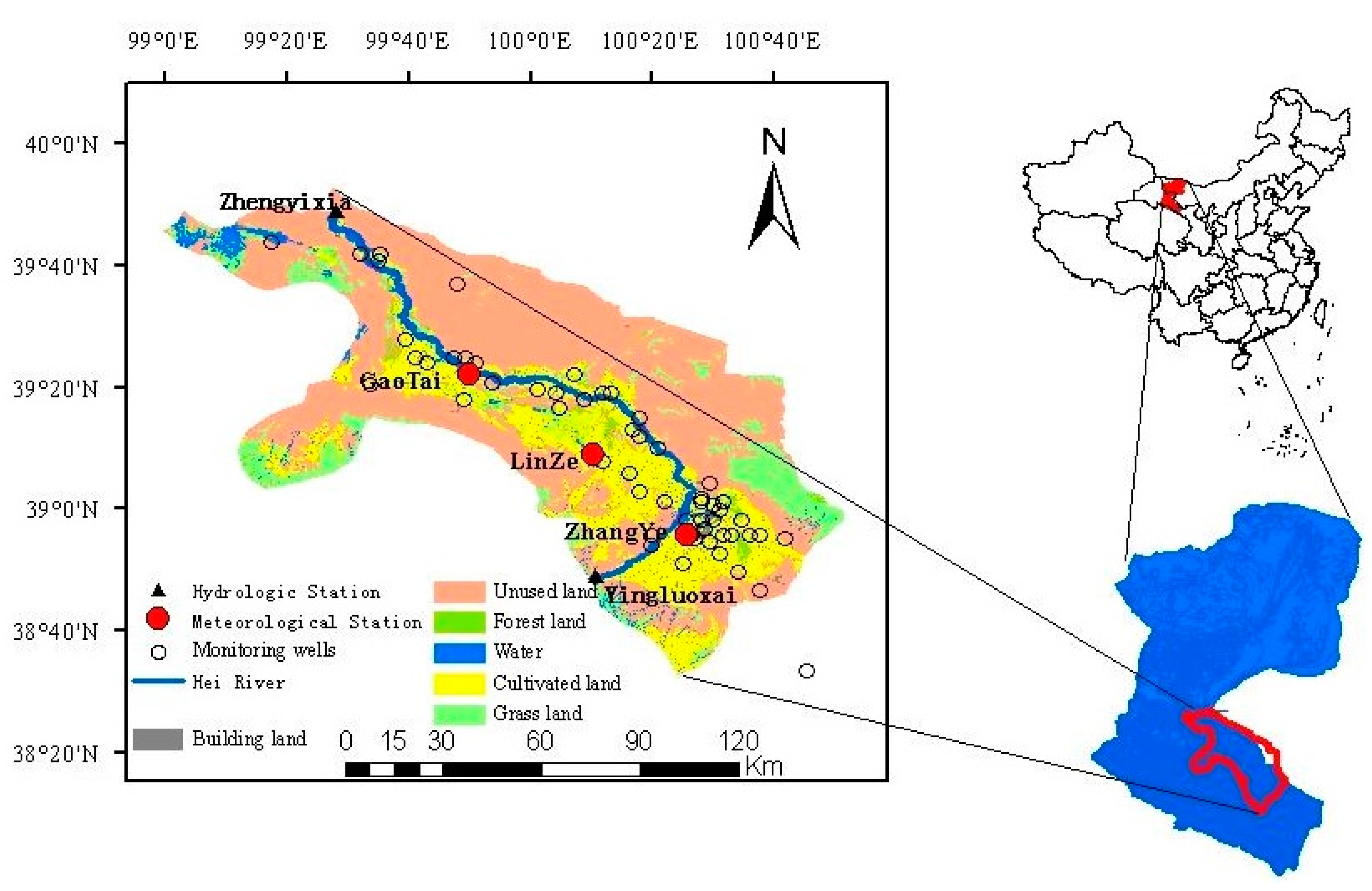
The study area occupied the middle reaches of the Hei River basin (38°30′–39°55′N, 98°55′–100°55′E; Figure 1), which is located in the middle of Hexi corridor of Gansu Province, northwest of China, and belongs to an arid climate zone. The total area is about 10,000 km2. The mean annual temperature is around 8 °C, the mean annual precipitation is between 69 and 216 mm and is concentrated between June and September, while the mean annual potential evaporation is between 1453 and 2351 mm [32].
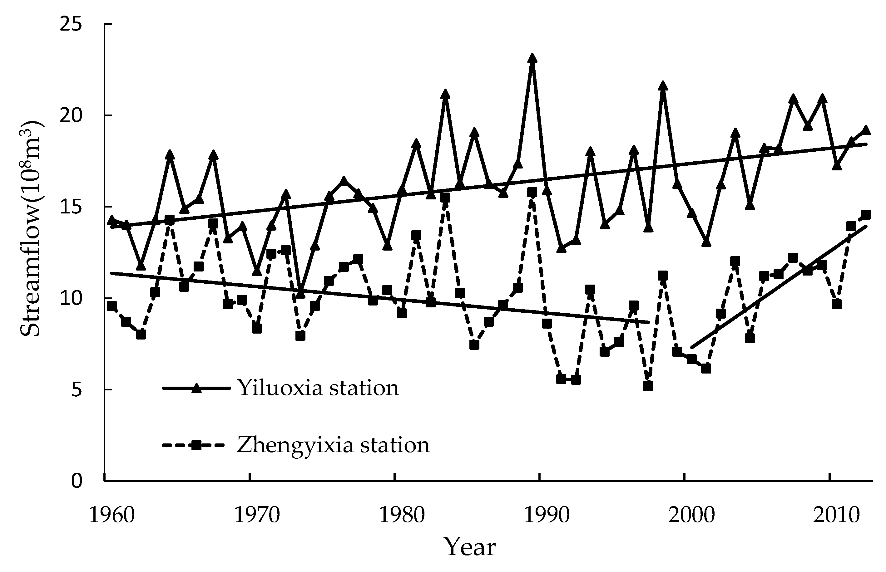
The Hei River is the second largest inland river in China with a total length of 821 km and a runoff of 16.0 × 10⁸ m3·year−1. It flows through Yingluoxia and Zhengyixia stations, entering and exiting middle reaches. Runoff has shown an increasing/decreasing trend in the past decade. The annual runoff at Yingluoxai station increased to 16.0 × 10⁸ m3 in the 1990s from around 14.4 × 10⁸ m3 in the 1960s (Figure 2), while the runoff at Zhengyixai station decreased by 3 × 10⁸ m3 during the same time period (Figure 2). This situation accelerated desertification within the northern parts of the basin [33,34]. In order to mitigate deteriorating ecosystems in the Hei River basin, an Ecological Water Diversion Project (EWDP) was initiated by the Chinese government in 2000 to ensure the delivery of water to the lower reaches for ecological water needs [35]. After that, runoff at Zhengyixia station has increased to levels not recorded since the 1960s [33,36]. The implementation of the EWDP alleviated the ecological deterioration in the lower reaches of the Hei River but aggravated the water resources shortage in the middle reaches. In order to meet the increasing demand for water resources, groundwater exploration provided an option. After 2004, the recharge of groundwater also increased due to the increase in precipitation, irrigation and runoff replenishment. The temporal variation in groundwater levels of the observation wells over the period from2001 to 2011 is shown in Figure 3c which shows a rising trend in groundwater level along the Hei River [37]. However, the water level in the region away from the river showed a declining trend.
The annual NDVI of each pixel was calculated by the annual maximum value of NDVI in order to eliminate the noise from the cloud and solar altitude. The Moderate-resolution imaging spectroradiometer (MODIS)-based NDVI products(MYD13A2 and MOD13A2)used for this study were acquired from the National Natural Science Foundation of China “Environmental and Ecological Science Data Center in the West of China (http://westdc.westgis.ac.cn/)” with a spatial resolution of 1 km and a temporal resolution of 1 day, groundwater depths of 53 wells were obtained from the National Natural Science Foundation of China “Hei River Project Data Management Center (http://westdc.westgis.ac.cn/)” while monthly precipitation and temperature datasets were acquired from the China Meteorological Network (http://data.cma.cn/), with a 0.5° spatial resolution, interpolated according to the observed data of 2747 stations in China.
The ordinary kriging method was employed to interpolate the observed values of ground water depths. For consistency regarding the NDVI spatial resolution, the interpolated groundwater table levels, precipitation, and temperature datasets were rescaled to a 1 km spatial resolution.
4. Results and Discussion
4.1. Variation of Hydrometeorological Variables and NDVI
During the period from2001 to 2011, both the average temperature and cumulative precipitation increased at the three hydrologic stations (Figure 3a,b). The temperature increases significantly at Gaotai station (p < 0.05). However, the trend of temperature increase is not obvious at another two stations. The distributions of cumulative precipitation and average temperature are shown in Figure 4a,b. Temperature gradually rises from south to north, while precipitation decreases were also observed. This is mainly determined by topography.
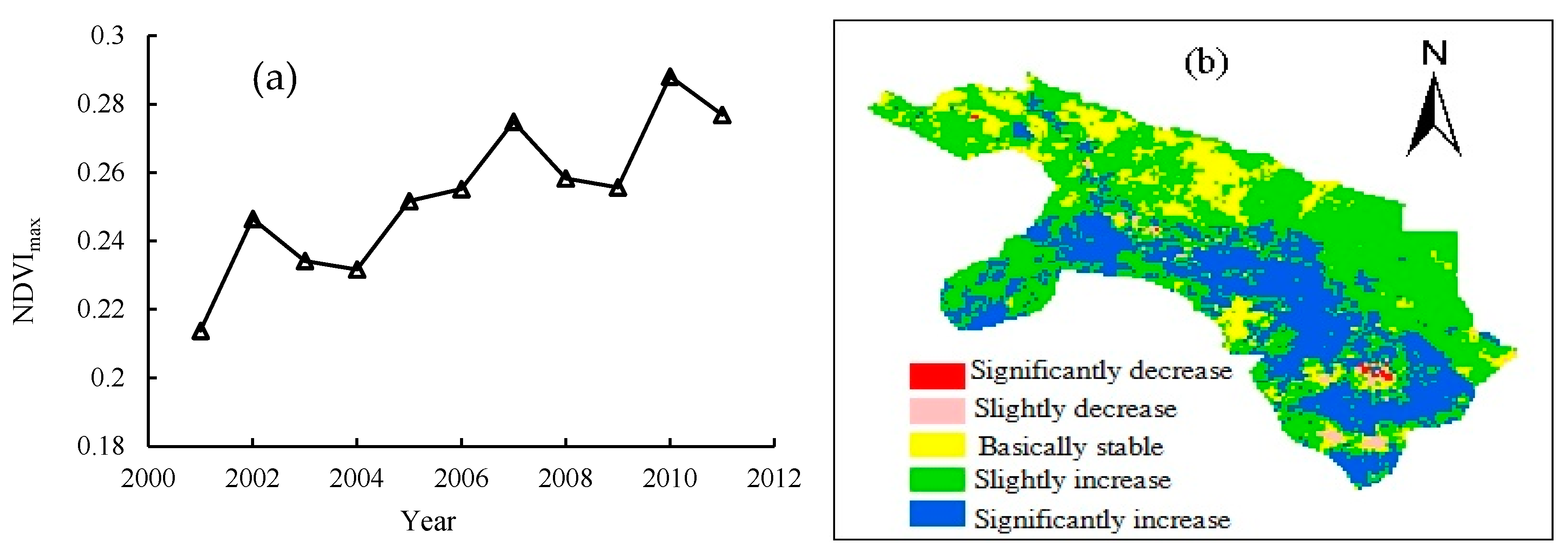
Figure 5a illustrates the annual maximum NDVI in the middle reaches of the Hei River basin from 2000 to 2011. The slope of the linear regression trend-line was 0.005. The NDVI time series corresponded to the average of all the pixels in the study area and reflected the overall trend. Figure 5b shows the spatial distribution of the linear regression slope (). In most cases, the area in which NDVI increased occupied about 94% of the total area. It can be seen that NDVI changes obviously. In order to explore the influencing factors on NDVI variation, the whole region was divided into 5 sub-regions based on the joint entropy method, and different regression models were constructed considering hydro-meteorological variables.
4.2. Mutual Information of NDVI with Coupling of Variables
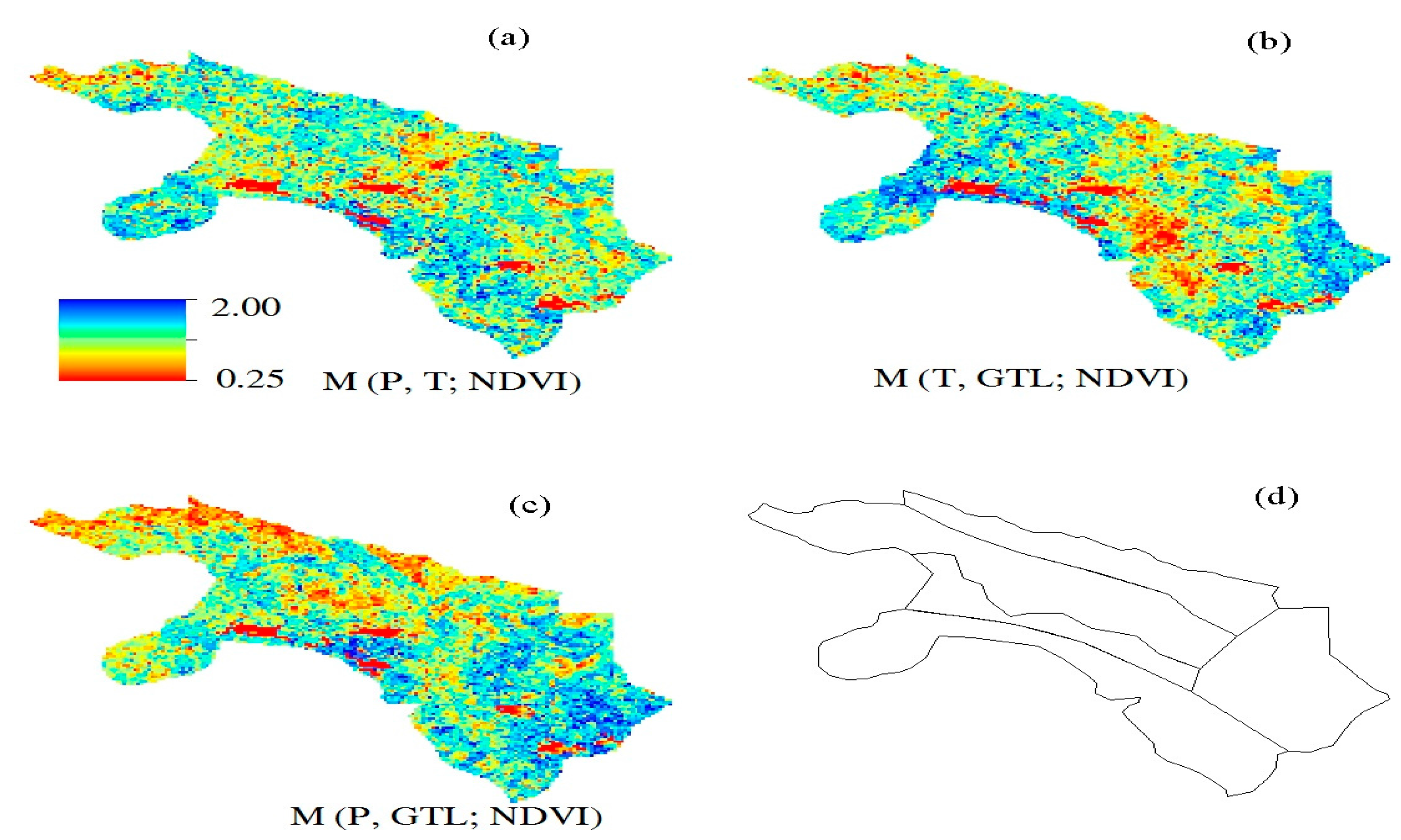
To understand the relationship between NDVI and hydro-meteorological variables, mutual information was employed to measure the dependence between the NDVI time series and each coupled variable. The greater the values of mutual information the higher the correlation. The spatial distribution of mutual information between NDVI and coupled variables are shown in Figure 6a–c, respectively. It can be observed from the figures that the mutual information of NDVI and coupled variables of precipitation and GTL generally decreased from southeast to northwest. The mutual information values of NDVI and the coupled variables of precipitation and temperature were dispersedly distributed, increasing from the center to the edge of regions, while the mutual information of NDVI and the coupled variables of temperature and groundwater table levels were greater in the northwestern and southeastern regions. In order to appropriately model the NDVI using dependent variables, the study region was artificially divided into 5 sub-regions (Figure 6d), based on three spatial distributions of mutual information, topographic and land use maps. In order to simply construct models, as far as possible each sub-region was made to have the same characteristics. For instance, sub-region I and sub-region IV are mainly mountainous and M (P, T; NDVI) is higher than M (T, GTL; NDVI) and M (P, GTL; NDVI) in most areas of these sub-regions. As the same time, the land use types are desert. Likewise, in most areas of sub-region II and sub-region V, M (GTL, P; NDVI) is higher than M (P, T; NDVI) and M (T, GTL; NDVI), and these areas are distributed as artificial oases.
4.3. Modelling NDVI
In sub-regions I and IV, precipitation and temperature were used to model the NDVI, since the mutual information of NDVI and the variables of precipitation and temperature were relatively higher. GTL and precipitation were used to model the NDVI in sub-regions II and V, while temperature and GTL were selected to model the NDVI in sub-region III.
Nested statistical models were developed for modeling NDVI in each sub-region. In most cases, the linear fitting of the NDVI time series to precipitation, temperature, and GTL resulted in poor correlation coefficients and high root means square error [17]. The vegetation growth may not be monotonic in relation to the atmospheric variables. For example, the temperature sensitivity of photosynthesis increases up to an optimum and later decreases as temperature gets higher [17]. A two-dimensional fitting was used to model NDVI using each of the hydro-meteorological variables as a factor. In order to select appropriate functional forms for modeling NDVI, four simple functional forms including linear function, quadratic function, exponent function and logarithm function were compared using Akaike information criterion (AIC) criteria. AIC is a measure of the relative quality of statistical models for a given set of data. The comparison of AIC values between different functional forms are as shown in Table 2. The smaller the AIC value, the more appropriate the form of the regression function. It was discovered that a logarithmic transformation of precipitation produced a better correlation with NDVI in some sub-regions (I, II, IV). Considering GTL and temperature, a negative exponential and a quadratic model showed a better relationship with NDVI. However, the logarithm regression model exhibited a better relationship between GTL and NDVI in sub-region III.
Different candidate equations were used to fit NDVI by coupling pair-wise precipitation, temperature, and GTL. The aim of the fitting procedures was to maximize the correlation coefficient and minimize the sum of squared residuals. However, the main importance of the fitting procedure was to maximize the proportion of the area in which the correlation coefficient met with significance testing.
In each sub-region, analysis was performed at the grid scale. In sub-regions I and IV, the coupling of precipitation and temperature resulted in a model of NDVI time series with an average correlation coefficient of 0.68 and 0.58, respectively. Li et al. (2016) also reported that in the desert regions in middle reaches of the Hei River, precipitation is a dominant influencing factor on annual NDVI variation [38]. Zhou et al. (2013) also demonstrated that precipitation and temperature are important factors driving the increase of NDVI in the study area [39]. However, the percentage of the area in which the correlation coefficient met with significance testing was only 42% (p < 0.05) and 15% (p < 0.01) in sub-region IV. This was mainly because the temperature was relatively high, thereby increasing evapotranspiration and water demand for vegetation growth that precipitation was unable to satisfy. In sub-regions II and V, the best fitting models were obtained by combining pair-wise negative exponentially transformed GTL respectively with the logarithmically and linearly transformed precipitation. In these regions, groundwater depths became an important influencing factor. Zhao et al. (2014) have also reported that in an oasis ecosystem, groundwater plays an important role in the formation of vegetation productivity [40]. In sub-region V, the percentage area in which the correlation coefficient met with the significance testing was only 50% (p < 0.05) and 16% (p < 0.01). There was a large area of arable land and artificial grassland in sub-region V (Figure 1). In sub-regions III and V, the growth of vegetation was strongly influenced by human activities, e.g., irrigation. Therefore, irrigation was the main influencing factor for vegetation growth. Beyond that, there was a considerable amount of water in sub-region III, thereby influencing prediction accuracy. After various fittings in different sub-regions, the correlation coefficients were combined for the entire study area (Figure 7). Results showed that there was about 53% of the area in which relationships were significant.
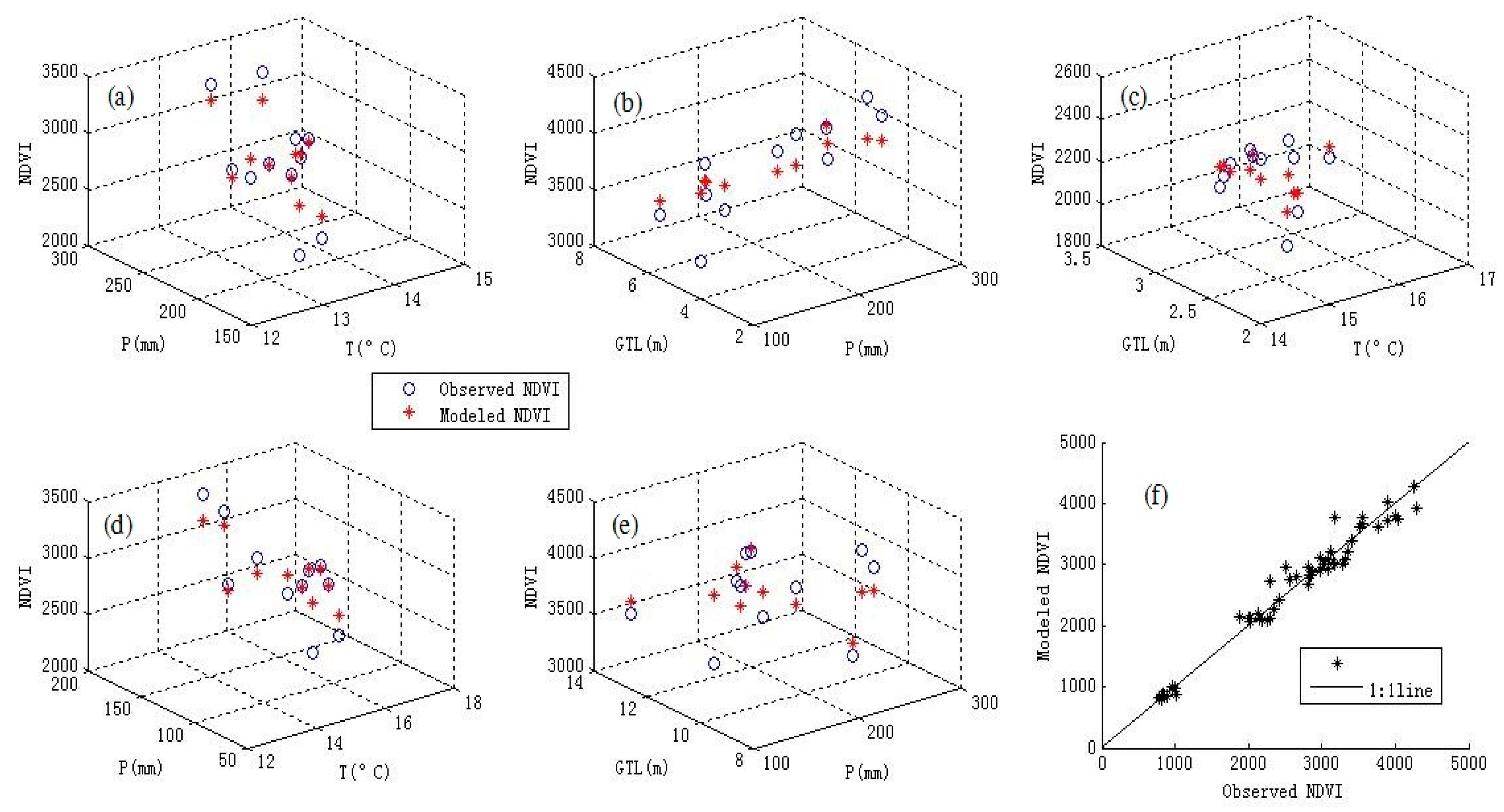
Analysis was also performed on a regional scale. Using the average NDVI time series of different sub-regions as predicted and each of the average hydro-meteorological variables as a predictor, a two-dimensional fitting was employed in the five sub-regions, respectively. This prediction also employed the same formulas used for the prediction on a grid scale (Table 3). Figure 8a–e showed the results of the three-dimensional scatter-plot couplings. Comparisons of these figures demonstrated that sub-regions I and II had a better accuracy of fitting. Figure 8f presents the overall relationship between observed NDVI and modeled NDVI for the whole region, where the correlation coefficient was observed to be 0.97, which indicated a high accuracy. This showed that this method was suitable for NDVI modeling.
5. Conclusions
In this study, the spatio-temporal variation of vegetation cover in the middle reaches of theHei River basin and the main driving factors during the period from 2001 to 2011 were analyzed using MODIS NDVI data and hydro-meteorological data. Considering the nonlinear relationship between hydro-meteorological variables, the entropy theory was employed to calculate the mutual information between the NDVI time series and coupled hydro meteorological variables. Based on the spatial distribution of mutual information, the whole region was further divided into 5 sub-regions, and nested statistical models were employed to simulate NDVI in each sub-region. The main conclusions are as follows:
- (1)
- The average annual NDVI increased at a rate of 0.005/a over the past 11 years in the middle reaches of the Hei River. The percentage area in which NDVI increased occupied 94% of the total area.
- (2)
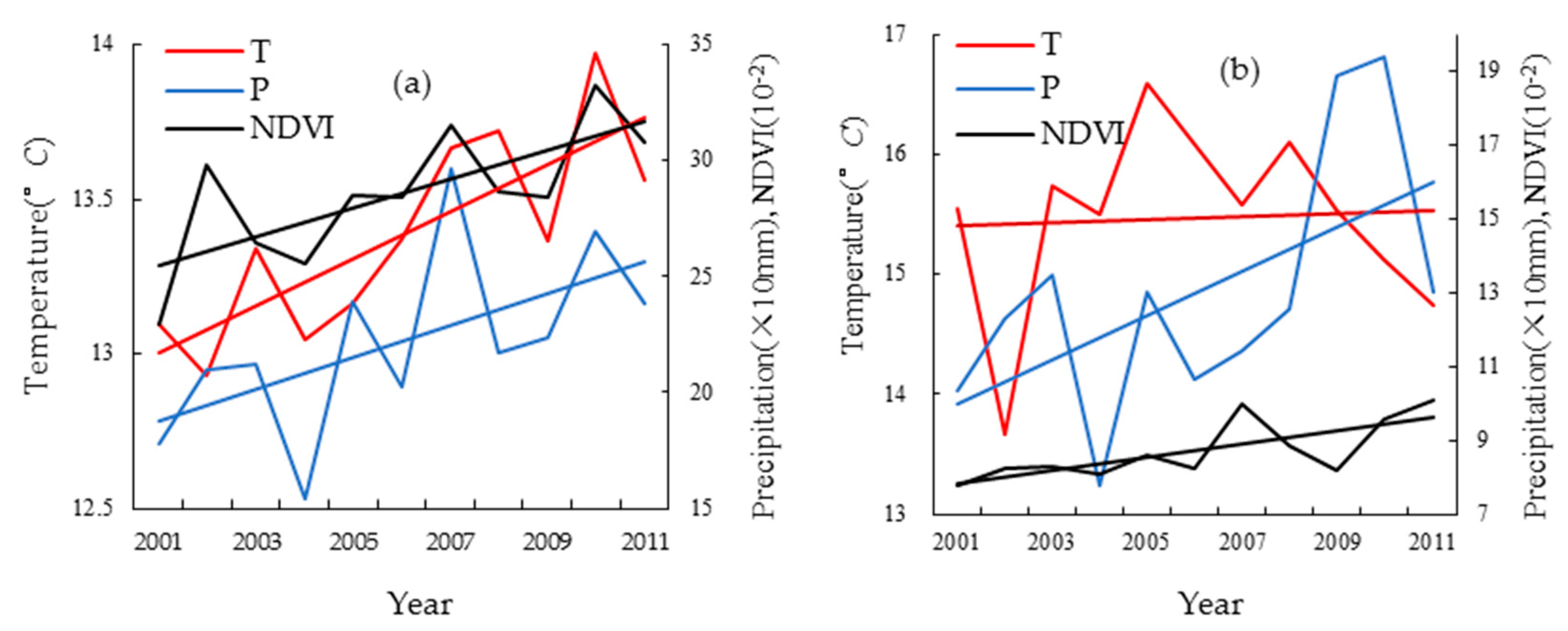
- In the desert sub-regions (I and IV), temperature and precipitation are the main driving factors for vegetation growth. In sub-region I, NDVI is consistent with the trend of temperature and precipitation (Figure 9a). However, in sub-region IV, the trend of temperature change is not obvious and the change in NDVI is mainly due to the increase in precipitation (Figure 9b). In the oasis regions (sub-region II and sub-region III), groundwater was an important factor for vegetation growth.
- (3)
- In coupling hydro-meteorological variables, a nested statistical model was proposed for modeling NDVI on a regional scale. The overall correlation coefficient between observed NDVI and modeled NDVI was observed to be 0.97. This high simulation accuracy further proves the suitability of this method.
- (4)
- Due to the influence of human activities, the modeling accuracy was not effective within the artificial oasis (sub-region III and sub-region V). For instance, in irrigation areas, vegetation can absorb water from irrigation to sustain growth but in non-irrigation areas the over-exploitation of groundwater caused by the increase in the amount of irrigation breaks the natural ecological balance, affecting the growth of natural vegetation. Additionally, the shortage of the dataset may also be a factor influencing the modeling accuracy. For instance, the scarcity of temperature and precipitation data may cause nearby cells to have similar values of T and P. Therefore, further studies are necessary for modeling NDVI that consider additional factors such as runoff and irrigation using long-term and higher resolution datasets.
The results can provide some scientific guidance for water resources management and the reasonable exploitation of groundwater, especially in the artificial oasis areas. The outcomes demonstrated the ability to successfully employ the joint entropy method in vegetation dynamics analysis in relation to hydro-meteorological variables.
Acknowledgments
We are grateful for the grant support from the National Natural Science Fund in China (91425302 and 51279166).
Author Contributions
Gengxi Zhang and Xiaoling Su designed the computations and wrote the paper; Vijay P. Singh and Olusola O Ayantobo revised the paper and gave some suggestions; All authors have read and approved the final manuscript.
Conflicts of Interest
The authors declare no conflict of interest.
References
- Kutiel, P.; Cohen, O.; Shoshany, M.; Shub, M. Vegetation establishment on the southern Israeli coastal sand dunes between the years 1965 and 1999. Landsc. Urban Plann. 2004, 67, 141–156. [Google Scholar] [CrossRef]
- Jin, X.M.; Liu, J.T.; Wang, S.T.; Xia, W. Vegetation dynamics and their response to groundwater and climate variables in Qaidam Basin, China. Int. J. Remote Sens. 2016, 37, 710–728. [Google Scholar] [CrossRef]
- Piao, S.L.; Mohammat, A.; Fang, J.Y.; Cai, Q.; Feng, J.M. NDVI-based increase in growth of temperate grasslands and its responses to climate changes in China. Glob. Environ. Chang. 2006, 16, 340–348. [Google Scholar] [CrossRef]
- Dai, S.P.; Zhang, B.; HaiJun, W.J.; Wang, Y.M. Vegetation cover change and the driving factors over northwest China. J. Arid Land 2011, 3, 25–33. [Google Scholar] [CrossRef]
- Liu, J.H.; Wu, J.J.; Wu, Z.T.; Liu, M. Response of NDVI dynamics to precipitation in the Beijing–Tianjin sandstorm source region. Int. J. Remote Sens. 2013, 34, 5331–5350. [Google Scholar] [CrossRef]
- Reed, B.C.; Brown, J.F.; Darrel, V.Z.; Loveland, T.R.; Merchant, J.W.; Ohlen, D.O. Measuring phenological variability from satellite imagery. J. Veg. Sci. 1994, 5, 703–714. [Google Scholar] [CrossRef]
- Clerici, N.; Weissteiner, C.J.; Gerard, F.G. Exploring the Use of MODIS NDVI-Based Phenology Indicators for Classifying Forest General Habitat Categories. Remote Sens. 2012, 4, 1781–1803. [Google Scholar] [CrossRef] [Green Version]
- Feilhauer, H.; He, K.S.; Rocchini, D. Modeling Species Distribution Using Niche-Based Proxies Derived from Composite Bioclimatic Variables and MODISNDVI. Remote Sens. 2012, 4, 2057–2075. [Google Scholar] [CrossRef]
- Rousvel, S.; Armand, N.; Andre, L.; Tengeleng, S. Comparison between vegetation and rainfall of Bioclimatic Ecoregions in Central Africa. Atmosphere 2013, 4, 411–427. [Google Scholar] [CrossRef]
- Xiao, J.F.; Zhou, Y.; Zhang, L. Contribution of natural and human factors to increases in vegetation productivity in China. Ecosphere 2015, 6, 1–20. [Google Scholar] [CrossRef]
- Nemani, R.; White, M.; Thornton, P.; Nishid, K.; Reddy, S.; Jenkins, J.; Running, S. Recent trends in hydrologic balance have enhanced the terrestrial carbon sink in the United States. Geophys. Res. Lett. 2002, 29, 1–4. [Google Scholar] [CrossRef]
- Brunsell, N.A.; Young, C.B. Land surface response to precipitation events using MODIS and NEXRAD data. Int. J. Remote Sens. 2008, 29, 1965–1982. [Google Scholar] [CrossRef]
- Kawabata, A.; Ichii, K.; Yamaguchi, Y. Global monitoring of interannual changes in vegetation activities using NDVI and its relationships to temperature and precipitation. Int. J. Remote Sens. 2001, 22, 1377–1382. [Google Scholar] [CrossRef]
- Pettorelli, N.; Pelletier, F.; Hardenberg, A.; Festa-Bianchet, M.; Cote, S.D. Early onset of vegetation growth vs. rapid green-up, Impacts on juvenile mountain ungulates. Ecology 2007, 88, 381–390. [Google Scholar] [CrossRef] [PubMed]
- Piao, S.L; Nan, H.J.; Huntingford, C.; Ciais, P.; Friedlingstein, P. Evidence for a weakening relationship between interannual temperature variability and northern vegetation activity. Nat. Commun. 2014, 5, 5018. [Google Scholar] [CrossRef] [PubMed] [Green Version]
- Pielke, R.A.; Avissar, R. Interactions between the atmosphere and terrestrial ecosystems, influence on weather and climate. Glob. Chang. Biol. 1998, 4, 461–475. [Google Scholar] [CrossRef]
- Sohoulande, D.C.; Singh, V.P. Retrieving vegetation growth patterns from soil moisture, precipitation and temperature using maximum entropy. Ecol. Model. 2015, 309, 10–21. [Google Scholar] [CrossRef]
- Ichii, K.; Kawabata, A.; Yamaguchi, Y. Global correlation analysis for NDVI and climatic variables and NDVI trends, 1982–1990. Int. J. Remote Sens. 2002, 23, 3873–3878. [Google Scholar] [CrossRef]
- Nicholson, S; Davenport, M. A comparison of the vegetation response to rainfall in the Sahel and East-Africa, using normalized difference vegetation index from NOAA AVHRR. Clim. Chang. 1990, 17, 209–241. [Google Scholar] [CrossRef]
- Jin, X.M.; Guo, R.H.; Zhang, Q.; Zhou, Y.X.; Zhang, D.R.; Yang, Z. Response of vegetation pattern to different landform and water-table depth in Hailiutu River basin, Northwestern China. Environ. Earth Sci. 2014, 71, 4889–4898. [Google Scholar] [CrossRef]
- Lv, J.J.; Wang, X.S.; Zhou, Y.X.; Qian, K.Z.; Wan, L.; Eamus, D.; Tao, Z.P. Groundwater-dependent distribution of vegetation in Hailiutu River catchment, a semi-arid region in China. Ecohydrology 2013, 6, 142–149. [Google Scholar] [CrossRef]
- Jin, X.M.; Schaepman, M.E.; Clevers, J.; Su, Z.B.; Hu, G.C. Groundwater Depth and Vegetation in the Ejina Area, China. Arid Land Res. Manag. 2011, 25, 194–199. [Google Scholar] [CrossRef]
- Mishra, A.K.; Ines, A.V.M.; Singh, V.P.; Asen, J.W. Extraction of information content from stochastic disaggregation and bias corrected downscaled precipitation variables for crop simulation. Stoch. Environ. Res. Risk Assess. 2012, 27, 449–457. [Google Scholar] [CrossRef]
- Singh, V.P. Entropy Theory and Its Application in Environmental and Water Engineering; Wiley: New York, NY, USA, 2013. [Google Scholar]
- Li, C.; Singh, V.P.; Mishra, A.K. Entropy theory-based criterion for hydrometric network evaluation and design, Maximum information minimum redundancy. Water Resour. Res. 2012, 48, 1–15. [Google Scholar] [CrossRef]
- Phillips, S.J.; Anderson, R.P.; Schapire, R.E. Maximum entropy modeling of species geographic distributions. Ecol. Model. 2006, 190, 231–259. [Google Scholar] [CrossRef]
- Pueyo, S.; He, F.; Zillio, T. The maximum entropy formalism and the idiosyncratic theory of biodiversity. Ecol. Lett. 2007, 10, 1017–1028. [Google Scholar] [CrossRef] [PubMed]
- Urbani, F.; Alessandro, P.; Frasca, R.; Biondi, M. Maximum entropy modeling of geographic distributions of the flea beetle species endemic in Italy (Coleoptera, Chrysomelidae, Galerucinae, Alticini). Zoologischer Anzeiger 2015, 258, 99–109. [Google Scholar] [CrossRef]
- Song, Y.; Ma, M. Varition of AVHRR NDVI and its relationship with climate in Chinese arid and cold regions. J. Remote Sens. 2008, 12, 499–505. [Google Scholar]
- Sohoulande Djebou, D.C.; Singh, V.P.; Frauenfeld, O.W. Analysis of watershed topography effects on summer precipitation variability in the southwestern United States. J. Hydrol. 2014, 511, 838–849. [Google Scholar] [CrossRef]
- McGill, W.J. Mutivariate information transmisson. Psychometrica 1954, 19, 97–116. [Google Scholar] [CrossRef]
- Nian, Y.; Li, X.; Zhou, J.; Hu, X. Impact of land use change on water resource allocation in the middle reaches of the Heihe River Basin in northwestern China. J. Arid Land 2013, 6, 273–286. [Google Scholar] [CrossRef]
- Wang, Y.; Roderick, M.L.; Shen, Y.; Sun, F. Attribution of satellite-observed vegetation trends in a hyper-arid region of the Heihe River basin, Western China. Hydrol. Earth Syst. Sci. 2014, 18, 3499–3509. [Google Scholar] [CrossRef]
- Guo, Q.; Feng, Q.; Li, J. Environmental changes after ecological water conveyance in the lower reaches of Heihe River, northwest China. Environ. Geol. 2009, 58, 1387–1396. [Google Scholar] [CrossRef]
- Zhang, A.; Zheng, C.; Wang, S.; Yao, Y. Analysis of streamflow variations in the Heihe River Basin, northwest China, Trends, abrupt changes, driving factors and ecological influences. J. Hydrol. Reg. Stud. 2015, 3, 106–124. [Google Scholar] [CrossRef]
- Qin, D.; Zhao, Z.; Han, L.; Qian, Y. Determinnation of groundwater recharge regim and flowpath in the Lower Heihe River basin in an arid area of Northwest China by using environmental tracers, Implications for vegetation degradation in the Ejina Oasis. Appl. Geochem. 2012, 27, 1133–1145. [Google Scholar] [CrossRef]
- Mi, L.; Xiao, H.; Zhang, J.; Yin, Z.; Shen, Y. Evolution of the groundwater system under the impacts of human activities in middle reaches of Heihe River Basin (Northwest China) from 1985 to 2013. Hydrogeol. J. 2016, 24, 971–986. [Google Scholar] [CrossRef]
- Li, F.; Zhao, W. Changes in normalized difference vegetation index of deserts and dunes with precipitation in the middle Heihe River Basin. Chin. J. Plant Ecol. 2016, 40, 1245–1256. [Google Scholar] [CrossRef]
- Zhou, W.; Wang, Q.; Zhang, C.B.; Li, J. Spatiotemporal variation of grassland vegetation NDVI in the middle and upper reaches of the Hei River and its response to climatic factors. Acta Prataculturae Sin. 2013, 22, 138–147. [Google Scholar]
- Zhao, W.; Chang, X. The effect of hydrologic process changes on NDVI in the desert-oasis ecotone of the Hexi Corridor. Sci. China Earth Sci. 2014, 57, 3107–3117. [Google Scholar] [CrossRef]
Figure 1.
Map of the middle reaches of Hei River basin and the monitoring wells.

Figure 2.
Annual discharge of Hei River at Yinluoxia and Zhengyixia stations.

Figure 3.
The temporal variation of average temperature of growing season (a); cumulative precipitation (b) and average ground depths (c).
Figure 3.
The temporal variation of average temperature of growing season (a); cumulative precipitation (b) and average ground depths (c).
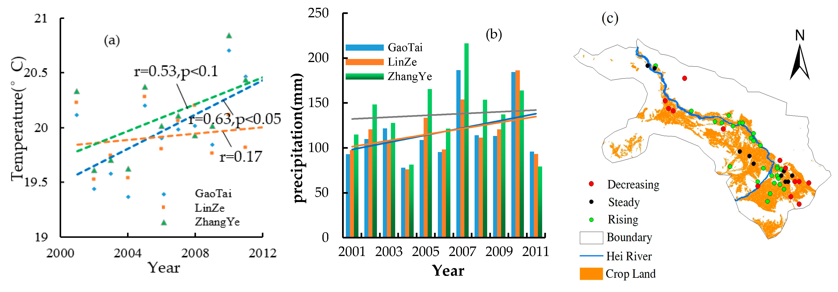
Figure 4.
The spatial distribution of (a) average temperature of growing season; (b) cumulative precipitation.
Figure 4.
The spatial distribution of (a) average temperature of growing season; (b) cumulative precipitation.
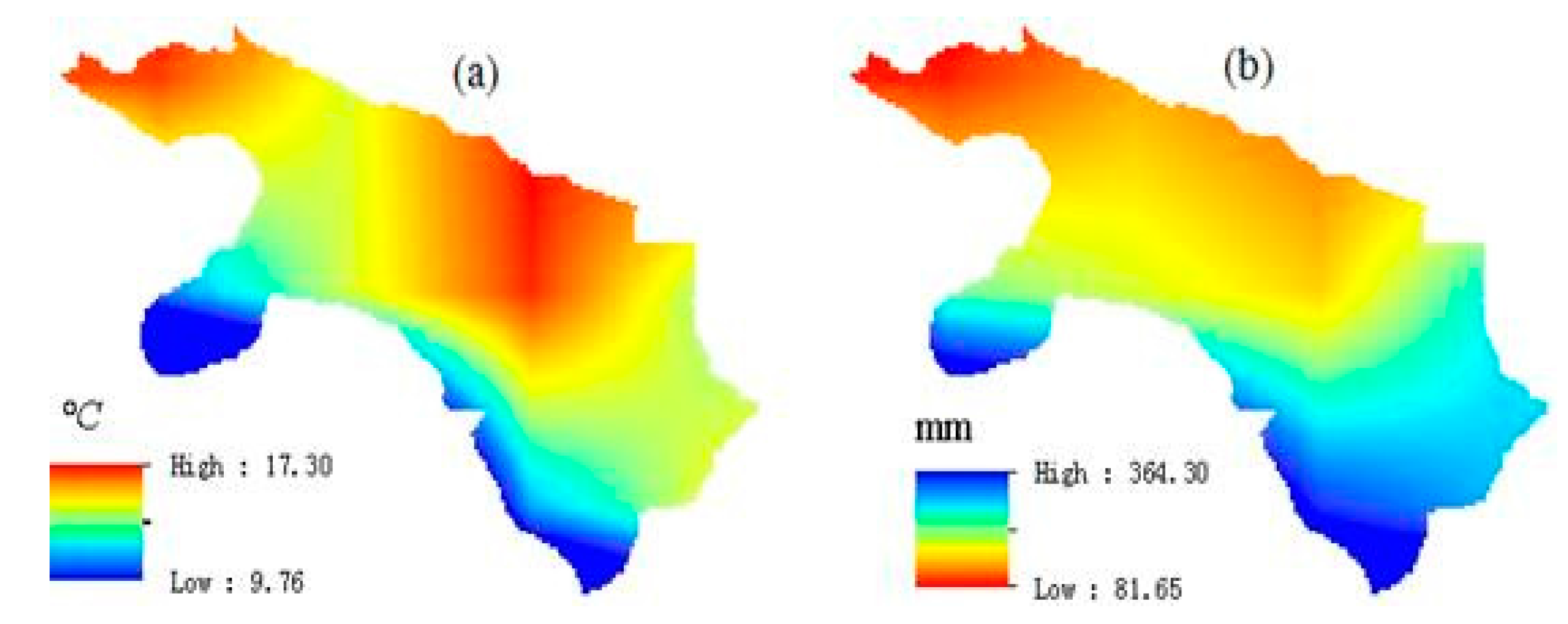
Figure 5.
Inter-annual variability of annual NDVI (a) and the trends of NDVI (b).

Figure 6.
The distribution of mutual information of NDVI and three coupling hydro-meteorological variables (a–c) and the divided sub-regions (d).
Figure 6.
The distribution of mutual information of NDVI and three coupling hydro-meteorological variables (a–c) and the divided sub-regions (d).

Figure 7.
The distribution of correlation coefficients of estimated NDVI by coupling hydro-meteorological variables.
Figure 7.
The distribution of correlation coefficients of estimated NDVI by coupling hydro-meteorological variables.
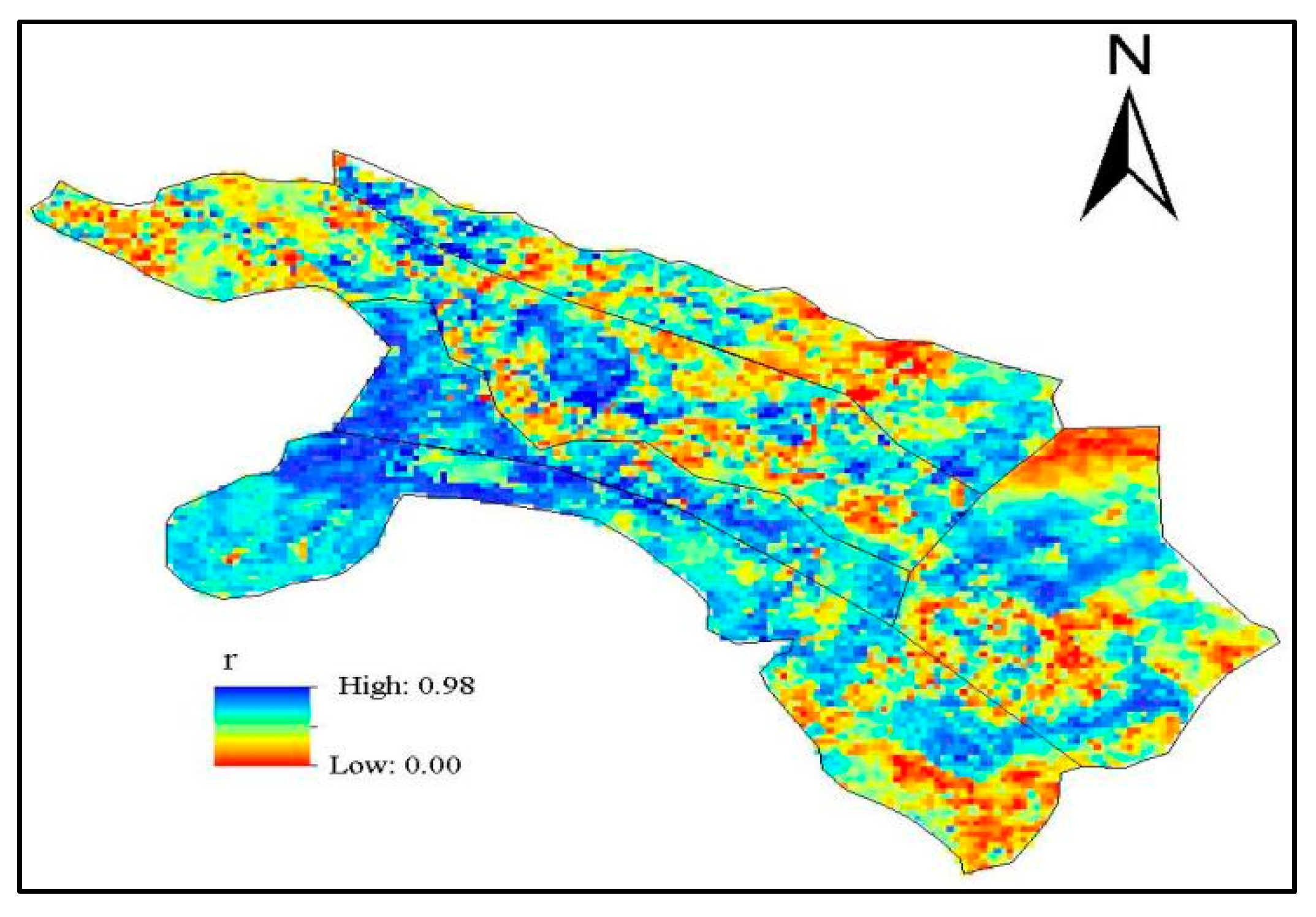
Figure 8.
Three-dimensional scatter plots of NDVI (multiplied by 104) in five sub-regions (a–e) and the relationship between observed NDVI modeled NDVI in the whole region (f).
Figure 8.
Three-dimensional scatter plots of NDVI (multiplied by 104) in five sub-regions (a–e) and the relationship between observed NDVI modeled NDVI in the whole region (f).

Figure 9.
The variation of NDVI, temperature and precipitation on region I (a) and region IV (b). Note: The black, red and blue lines express the trend of variation in NDVI, temperature and precipitation respectively.
Figure 9.
The variation of NDVI, temperature and precipitation on region I (a) and region IV (b). Note: The black, red and blue lines express the trend of variation in NDVI, temperature and precipitation respectively.

Table 1.
Illustration of a three-dimension contingency employed to compute the joint PDF. Consider 3 variables X, Y, and Z.
Table 1.
Illustration of a three-dimension contingency employed to compute the joint PDF. Consider 3 variables X, Y, and Z.
| Variables | Discrete Probabilities | ||
|---|---|---|---|
| X = {X1,X2} | Y = {Y1,Y2} | Z = {Z1,Z2} | |
| X = X1 | Y = Y1 | Z = Z1 | p(X = X1, Y = Y1, Z = Z1) |
| Z = Z2 | p(X = X1, Y = Y1, Z = Z2) | ||
| Y = Y2 | Z = Z1 | p(X = X1, Y = Y2, Z = Z1) | |
| Z = Z2 | p(X = X1, Y = Y2, Z = Z2) | ||
| X = X2 | Y = Y1 | Z = Z1 | p(X = X2, Y = Y1, Z = Z1) |
| Z = Z2 | p(X = X2, Y = Y1, Z = Z2) | ||
| Y = Y2 | Z = Z1 | p(X = X2, Y = Y2, Z = Z1) | |
| Z = Z2 | p(X = X2, Y = Y2, Z = Z2) | ||
Note: Each variable is categorized into 2 classes (n = 2).
Table 2.
The comparison of AIC values between different functional forms on 5 sub-regions; AIC in bold indicates most appropriate functional form.
Table 2.
The comparison of AIC values between different functional forms on 5 sub-regions; AIC in bold indicates most appropriate functional form.
| NDVI and Temperature | ||||||
| Region | Region I | Region II | Region III | Region IV | Region V | |
| Function | ||||||
|---|---|---|---|---|---|---|
| liner | −3.6153 | −4.7407 | −6.1732 | |||
| quadratic | −3.8733 | −5.4122 | −6.5508 | |||
| exponent | −0.6537 | −1.3973 | −2.9187 | |||
| logarithm | −3.7049 | −5.2447 | −6.5427 | |||
| NDVI and Groundwater | ||||||
| Region | Region I | Region II | Region III | Region IV | Region V | |
| Function | ||||||
| liner | −1.8812 | −3.8162 | −2.7076 | |||
| quadratic | −3.8876 | −5.1042 | −4.3212 | |||
| exponent | −3.9708 | −2.2641 | −4.3329 | |||
| logarithm | 0.3744 | −5.1401 | 0.4571 | |||
| NDVI and Precipitation | ||||||
| Region | Region I | Region II | Region III | Region IV | Region V | |
| Function | ||||||
| liner | −3.5757 | −1.7001 | −4.9864 | −2.8516 | ||
| quadratic | −4.5808 | −4.714 | −7.1646 | −4.4654 | ||
| exponent | −4.5530 | −4.5093 | −7.1620 | −4.4443 | ||
| logarithm | −4.7402 | −4.7974 | −7.2847 | −2.5677 | ||
Table 3.
Fitting models, correlation coefficients and area proportion meeting significance testing in five sub-regions.
Table 3.
Fitting models, correlation coefficients and area proportion meeting significance testing in five sub-regions.
| Sub-Region No. | Fitting Formula | Average Correlation Coefficient | Area Proportion | Area Proportion |
|---|---|---|---|---|
| (p < 0.05) | (p < 0.01) | |||
| I | 0.68 | 0.75 | 0.40 | |
| II | 0.66 | 0.72 | 0.42 | |
| III | 0.47 | 0.36 | 0.16 | |
| IV | 0.58 | 0.42 | 0.15 | |
| V | 0.57 | 0.50 | 0.16 |
© 2017 by the authors. Licensee MDPI, Basel, Switzerland. This article is an open access article distributed under the terms and conditions of the Creative Commons Attribution (CC BY) license (http://creativecommons.org/licenses/by/4.0/).
Share and Cite
MDPI and ACS Style
Zhang, G.; Su, X.; Singh, V.P.; Ayantobo, O.O. Modeling NDVI Using Joint Entropy Method Considering Hydro-Meteorological Driving Factors in the Middle Reaches of Hei River Basin. Entropy 2017, 19, 502. https://doi.org/10.3390/e19090502
AMA Style
Zhang G, Su X, Singh VP, Ayantobo OO. Modeling NDVI Using Joint Entropy Method Considering Hydro-Meteorological Driving Factors in the Middle Reaches of Hei River Basin. Entropy. 2017; 19(9):502. https://doi.org/10.3390/e19090502
Chicago/Turabian StyleZhang, Gengxi, Xiaoling Su, Vijay P. Singh, and Olusola O. Ayantobo. 2017. "Modeling NDVI Using Joint Entropy Method Considering Hydro-Meteorological Driving Factors in the Middle Reaches of Hei River Basin" Entropy 19, no. 9: 502. https://doi.org/10.3390/e19090502
Note that from the first issue of 2016, this journal uses article numbers instead of page numbers. See further details here.