Paths of Cultural Systems


Owner and Operator, Ballonoff Consulting, 9307 Kings Charter Drive, Richmond, VA 23116, USA
Entropy 2018, 20(1), 8; https://doi.org/10.3390/e20010008
Submission received: 6 November 2017
/
Revised: 9 December 2017
/
Accepted: 17 December 2017
/
Published: 25 December 2017
(This article belongs to the Special Issue Quantum Probability and Randomness)
Abstract
:A theory of cultural structures predicts the objects observed by anthropologists. We here define those which use kinship relationships to define systems. A finite structure we call a partially defined quasigroup (or pdq, as stated by Definition 1 below) on a dictionary (called a natural language) allows prediction of certain anthropological descriptions, using homomorphisms of pdqs onto finite groups. A viable history (defined using pdqs) states how an individual in a population following such history may perform culturally allowed associations, which allows a viable history to continue to survive. The vector states on sets of viable histories identify demographic observables on descent sequences. Paths of vector states on sets of viable histories may determine which histories can exist empirically.
1. Ethnographic Foundation
The structures described here and their consequences imply much of what may be predicted about empirical cultures. Anthropologists very often draw illustrations of structures using methods discussed here, but based on intuition, thus have little notion of what their commonly used diagrams might predict. While [1,2] defined mathematical means to describe the current and future demographic organization of lineage organizations, with empirical examples, we here specify the demography of kinship-based systems [3,4,5,6,7,8] with some related definitions in our Appendix A; and empirical examples in [9,10,11,12,13]. We follow the inspiration of [14]. In an empirical culture many other relations may also occur; we note some of those in our Part 7, Discussion at the end.
Our notion of studying viable minimal structures—which are the smallest minimal cultural structures that can “reproduce” the ascribed social relations in one generation—follows from [15]. Our history describes how sustaining those relations allow the culture to reproduce the rules. Cultural rules describing histories may be stated in natural languages, which label the individuals in a descent sequence with a subset called a kinship terminology. Our term viable embodies what anthropologist Radcliff-Brown called “persistent cultural systems” ([10], p. 124). Radcliff-Brown and others often described histories using discrete generations, as do we. Empirical cultures are almost ubiquitously described by many anthropologists using viable histories, typically represented in an ethnography by its minimal structure. The nearly ubiquitous presence in ethnographies of viable histories implies they may be the only observed histories.
An example is Figure 1 (whose source is [9]) which is an actual viable minimal structure of a history (that is, a persistent cultural system). The triangles in the illustration are males, the circles are females, descent moves in the downward direction, the labels are names used in the kinship terminology. The sign “=” means “marriage” between the two individuals attached to it; the “=” on the far right in the illustration shows a marriage to the partner on the far left in each generation. The horizontal line which connects two individuals shows that those two are assigned descendants of the marriage above them. The fifth generation in this illustration is equal to the first (by its labels in vertical descent in the diagram), showing that minimal structure shown here reproduces the labelled culture here in four generations, but reproduces the minimal structure (the graphs without the kinship labels) in each generation. This minimal structure has 4 marriages in each generation hence has structural number s = 4. The minimal structure is not intended to illustrate the actual empirical relations of each empirical generation of individuals, instead it shows “how the rule operates”—it describes the minimal representation of the kinship and marriage rules (see Appendix A Definitions A3). The minimal structure describes the “principles” used in the rules of the culture.
Figure 1 is also obviously an example of a group. Claude Levi-Strauss [9] initially used groups to demonstrate histories in an appendix by A. Weil. Ref. [9] mainly discusses groups of orders 2, 4 and 8, though its illustration 1.17 shows a helical structure of order 4. Other studies include orders 3, 6 and others. Ref. [16] also shows a helical structure of order 7; helical minimal structures are also groups and have surjective descent sequences, so our modal demography discussed in [8] and Appendix A Definition A7 also apply to helices.
2. Basic Definitions
While lineage organizations [1,2] predicted examples of population measures including the “local” village size given the lineage structure, the kinship examples described here use values found in [8] to predict values associated to the structural number of the history, which apply no matter what the empirical size of the total population (so long as it is at or above the minimal size). Our definitions are stated in our Appendix A from previous articles (see also Appendix A) and those below.
Definition 1.
Let D be a finite non-empty set (called a dictionary) and let * be a partially defined binary operation on D, such that when x, y ∈ D:
- (1)
- If there exists an a ∈ D such that a*x and a*y are defined and a*x = b and a*y = b then x = y, we call such object (D, *) a partially defined quasigroup, or pdq.
- (2)
- If (D, *) is a pdq and * is fully defined on D, then (D, *) is a (complete) quasigroup.
- (3)
- The pair L = (D, *) is a natural language with dictionary D whenever (D, *) is a pdq.
- (4)
- If L = (D, *) is a natural language, a kinship terminology is a quasigroup subset k ⊆ L.
Definition 2.
Let X, Y and Z be non-empty finite sets and let (X, *), (Y, °) and (Z, ▪) be quasigroups with binary relations *, ° and ▪ respectively. Then:
- (1)
- A function f: X → Y is a homomorphism if f for all b, c ∈ X, f(b * c) = f(b) ° f(c).
- (2)
- If f: X → Z and g: Y → Z are homomorphisms then f and g are isotopic.
All empirical languages are natural languages [7]. Under Definition 2(2) if Y and Z are isotopic they are also istotopic dictionaries: two possibly different descriptions, thus typically of distinct natural languages, of the “same” objects or illustrations. Our definition of kinship terminologies based on quasigroups follows from [17], which refined the discussion of Weil in [9]. While empirical kinship systems are non-associative [18], a large class is associative and complete, form finite permutations, indeed groups [19,20,21] hence form kinship terminologies as defined here. Groups thus arise in anthropology because a set of all 1-1 mappings of a finite subset set k of a quasigroup (a kinship terminology k) onto itself forms a group (the symmetric group on k). If (X, *), (Y, °) and (Z, ▪) are complete pdqs then (isotopic) homomorphisms classify kinship terminologies by the form of the pdq onto which they are mapped. For example, the isotopic terminologies classified as Dravidian [12,22,23] and others are often discussed, in part because they have interesting group theoretical structures.
Definition 3.
Let H be a non-empty finite set of viable histories. Let G be a non-empty descent sequence using H, let Gt ∈ G be a generation of G at t, and let Ht ⊆ H be a subset of t. Then then for each α ∈ Ht, the real numbers 0 vα(t) 1 such that Σαvα(t) = 1 is the vector state of Gt.
Adopting a standard order for listing the histories, we write the vector state at t as v(t) := (vα(t), …, vχ(t)), or when |Ht| = h, as v(t) = (v1(t), …, vh(t)). Let H be a finite non-empty set of viable histories, let α ∈ H, let Gt ∈ G be a generation of G, and let v(t) be the vector state of Gt (see also Appendix A Definitions A2–A5). Then:
- From [2,5,6,8] and Appendix A Definition A4 each structural number s has a set of values ns and ps where nsps = 2, where ns is the average family size of a pure system of structural number s and ps is the proportion of reproducing adults of a pure system of structural number s. If history α has structural number s, then each α has modal demography (nα, pα) = (ns, ps) (see Appendix A Definition A7) where ps = 2/ns; for s ≥ 3 and sα ≠ sχ then (nα, pα) ≠ (nχ, pχ).
- Since H is finite, each non-empty set of viable histories H thus has a largest structural number smax with modal demography (nmax, pmax), and a smallest structural number smin with modal demography (nmin, pmin). Note that if nmax increases then pmax decreases (and as nmin decreases then pmin increases, since given s, nsps = 2, with 0 < p ≤ 1. Structural numbers s = 2 or 3 have identical modal demography (ns, ps) = (2, 1); all others structural numbers have distinct modal demographies see [5,8].
- The modal demography of history α with structural number sα is (nα, pα) = (ns, ps) is a set of values that represent the history α maintaining its modal demography with neither increase nor decrease in total empirical population size; it is prediction of nα and pα based on the determination that the structural number is s, and maintains the structural number s.
- n(t) = Σαvα(t)nα, α ∈ H, is the predicted average family size of Gt at t, given the vector state at t see [8]. Note that this is the average family size of the population at time t, given the vector state of each α ∈ Ht. This while the “size” of the minimal structure might be small, the size predicted by n(t) is the predicted actual size of the total population at t, not of the minimal structure; the minimal structure illustration “size” is dependent on the rules, not on the empirical size of the population.
- p(t) = Σαvα(t)pα, α ∈ H, is the predicted proportion of reproducing adults of Gt at t ascribed as married and reproducing, given the vector state of sα at t [8].
- Thus, all of the “demographics” of cultural theory discussed here are predictions on the result of maintaining or changing the vector states of t, given the SNSK determined values for each modal demography (nα, pα) at time t. Thus, [8] defineswhere r(t) ∈ R predicts an average rate of change of total population size between two generations of G, based on the vector state of structural numbers of the histories Ht ⊆ H. [8] showed that r(t) predicts changes in the probabilities v(t) imply cultural change is adiabatic.er(t) = 1/2n(t)p(t)
- Let H be a finite non-empty set of viable histories, and α, χ ∈ H. Using vα(t) = 1 − vχ(t), nα = 2/pα and nχ = 2/pχ, then Equation (1) becomeswhere:er(t) = 1 + (nαχ – 2)vα(t) + (2 – nαχ)vα(t)2is a constant determined by the values of nα and nχ; note nαχ = nχα.nαχ := (nα2 + nχ2)/(nαnχ)
3. Paths of Descent Sequences
Definition 4.
Let H be a finite set of non-empty viable histories. Let α, χ, etc ∈ Ht ⊆ H and let the structural number of α ≠ χ, etc. If for any such set, |Ht| > 1, vt(α) = 1 or 0, then H is not full; otherwise H is full.
Definition 5.
If H is a finite non-empty set of viable histories, then F ⊆ H is a face of H see [2,4,8]. Let I = [1, 0]. A path from point a to point b in a set X is a function f: I → X with f(0) = a and f(1) = b, in which case a is called the initial point of the path and b is called the terminal point of the path. Given a path, in case a = b then such path is a closed path. If [x, y] ∈ I and f(x) = a and f(y) = b then f[x, y] is called an interval and a sub-path of I. A reverse path from point a to point b in X is a function f: I → X with f(1) = a and f(0) = b. Given a path (or reverse path) from t0 to t1, if t1 ≥ tk ≥ t0 we say that tk is in the path.
Lemma 1.
Let Ht be a finite non-empty set of full viable histories and α, χ ∈ Ht. Then:
- 1.
- r(t) ≥ 0, and r(t) = 0 if all structural numbers have the same modal demography or if all have structural numbers 2 or 3.
- 2.
- If α and χ are distinct structural numbers and at least one has structural number >3, then r(t) > 0 and r(t) has a maximum at v(t) = (0.5, 0.5).
- 3.
- Given any finite non-empty set H of two or more viable histories, there is a unique maximum r(t), given by (ii).
Proof 1.
Assume first the modal demographies of histories α and χ are equal (which occurs if sα = sχ or if sα, sχ < 4). Then nα = nχ. Then nαχ = 2, so the sum in Equation (2) is er(t) = 1, or r(t) = 0. Assume now sα ≠ sχ and at least one structural number is >3, so the modal demographies of α and χ are distinct, and we do not have vα(t) = 0 or 1. Then in Equation (2) (nαχ − 2) = −(2 − nαχ), but vα(t) > 0, so then vα(t) > vα(t)2. Thus, (nαχ − 2)vα(t) > (2 − nαχ)vα(t)2, so Equation (2) states r(t) > 0. ☐
Proof 2.
To show r(t) has a maximum when v(t) = (0.5, 0.5), we use the first two terms of a Taylor expansion from (1) to find er(t) = 1 + r(t). Differentiating twice gives a2 exp[r(t)]/δy2 = 2 − 2nαχ where y = v(t). When sα ≠ sχ and at least one of sα, sχ is > 3, nαχ > 2, then exp[r(t)] is concave down; so, r(t) is also concave down. ☐
Proof 3.
There is a finite number of two-history pairs in H. Since ns increases as s increases, then Lemma 1 part 1 shows that the largest value of r(t) will be set by that two-history subset α, χ of H having the largest difference between their structural numbers, hence the largest nαχ in Equation (3). Combining the ns of the largest s with any other combination of ns values will result in a smaller nαχ hence smaller er(t), from Equation (3). ☐
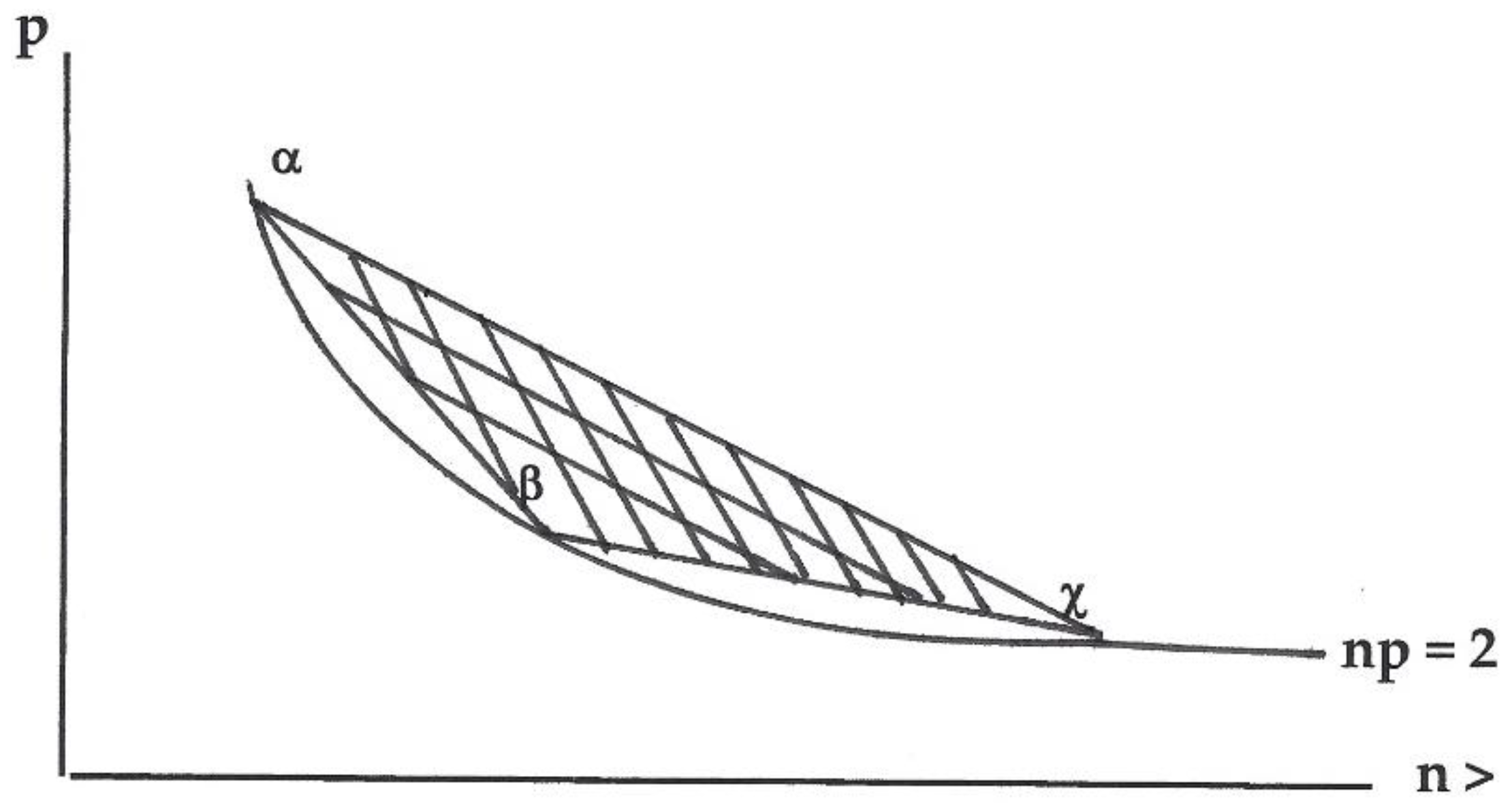
Observation 1.
Assume a finite non-empty set of viable histories H acting on a finite non-empty descent sequence G. Let α, β, χ ∈ Ht ⊆ H act on generation Gt ∈ G. See Figure 2:
The curved bottom-line in Figure 2 is the locus wherever np = 2, so includes the modal demography of each history in H; that is, the modal demography for each of α, β and χ each appear on the line np = 2, since nsps = 2. If for any α, vα(t) = 1, then n(t) = nα, p(t) = pα, so er(t) = ½n(t)p(t) = ½nαpα = ½2 = 1 so r(t) = 0; this occurs if all histories in Ht have the same structural number (or all have structural numbers 2 and 3). When that does not occur we have a set of two or more histories in Ht each with 0 < vα(t) < 1 and thus r(t) > 0; see also Lemma 1. When H is full, assume α, β and χ have distinct structural numbers, at least two of α, β, χ have structural numbers >3, and α is has the lowest structural number of those three histories. Then the modal demography of α, β, χ have (nα, bα) ≠ (nβ, bβ) ≠ (nχ, bχ), and the computation of r(t) appears in the values in the triangle area of Figure 2. However, if Ht is not full then events in the triangle area might not occur. Even if paths allow α with β, α with χ and β with χ (thus the boundaries of the triangle area), values of r(t) within the triangle only occur if all three histories are allowed by H, which may be prohibited by not-full H. We call such area an un-accessed region. Thus, we study change using both full and non-full sets of histories.
4. Pictures of States on Descent Sequences
Definition 6.
Let H be a finite non-empty set of histories and let (nα, pα) be the modal demography for history α ∈ H. Let G be a finite non-empty descent sequence using H, and let Gt ∈ G be the generation at time t. Let Ht be a face of H specified at t. Let St := { sα|α ∈ Hi} be the set of structural numbers St ⊆ S of histories Ht available at t. Let At := {(nα, pα)|sα ∈ Si, α ∈ Hi, (nα, pα) = (ns, ps)} be the set of modal demographies At of the histories in Ht; and let v(t) be the vector state of Gt. List the histories in H in a defined order from α to χ. Then for all α ∈ Ht and all (nα, pα) ∈ At, let:
- 1.
- (nt|:= (nα, …, nχ) be a row vector;
- 2.
- |pt) := (pα,…, …, pχ) be a column vector;
- 3.
- for all α, χ∈ H, arranging the sum of the inner product (nt|pt) as a square matrix then for all α, χ∈ H, H(t): = [nαpχ] is a demographic picture (analogous to a Heisenberg picture in physics) at t;
- 4.
- the square matrix we get by arranging the products of v(t)v(t)T as V(t) := [vαχ(t)] is a probability picture (analogous to a Schroedinger picture in physics) of the vector state of a descent sequence at t;
- 5.
- for ε ≥ 0 let V(Δ(t)) := V(t + ε) − V(t) = [vαχ(t + ε) − vαχ(t)] := [Δαχ(t)]. (Notice that −1 ≤ Δαχ(t) ≤ 1).We note [25] for our analogy of terminology.
Then for all α, χ ∈ H we can rewrite Equation (1) as:
using a probability picture which focuses on the vector states; and
using a demographic picture which focuses on demographic properties of the histories.
er(t) = ½ (n|V(t)|p)
er(t) = ½v(t)H(t)v(t)T
5. Comments on Demographic Pictures
Given a finite non-empty set of full viable histories H, observing a face Ht ⊆ H at t produces a list of the available Ht ⊆ H and thus creates a list of possible modal demographies (nα, pα) ∈ At for all α ∈ Ht. Let |Ht| = h. List the h histories in a fixed order from α to χ, with row vector (nt| = (nα, …, nχ) and column vector |pt) = (pα, …, pχ)T. So for histories α, …, χ ∈ Ht, we can write the demographic picture for |Ht| = h at t as (nt|pt) = H(t) where:
Each diagonal entry = 2 because a diagonal entry nαpα is determined by the modal demography (ns, ps) for each history, and nsps = 2. Thus, using ½H(t) we can restate Equation (5):
Because the two-history case has some useful properties, we present much of our discussion on the two history version, which becomes:
Lemma 2.
Let H be a finite non-empty set of full viable histories. Let G be a non-trivial descent sequence using H, let Ht ⊆ H be the face of H observed at t, and let G(t) ∈ G be the generation at t with vector state v(t). Then r(t) = 0 only if ½H(t) = [1] at all entries.
Proof of Lemma 2.
Assume the premises. Equations (4)–(7) simply rearrange terms in ½ΣiΣjvi(t)vj(t)nipj. From the definition of modal demography, pi = 2/ni and pj = 2/nj. The values on the diagonal of ½H(t) are for each history α, ½nαpα = 1. We thus examine the off-diagonal products nαpχ and nχpα. Then nipj = 2ni/nj and njpi = 2nj/ni. Thus, 2ni/nj = 2nj/ni occurs only if ni = nj, in which case nipj = njpi = 2. This occurs only if all histories i and j have the same structural number or both have s = 2 or 3, and thus ½H(t) = [1] in all entries. Otherwise stated, in this case the value from Equation (3) is nαχ = 2. ☐
Implications of Lemma 2: knowing the modal demography of histories in H we can compute a proposed population growth rate r(t).
- The result nα = nχ occurs if structural numbers sα, sχ are <4 or whenever sα = sχ; so r(t) = 0. Otherwise, then Lemma 2 implies Lemma 1, which says that er(t) ≠ 1, and thus r(t) > 0. This occurs since nαpχ does not equal nχpα; thus from Lemma 1 and [8] the off-diagonal elements of ½H(t) implies adiabatic change in r(t).
- In discussions in physics, when nαpχ ≠ nχpα some claim that the resulting r(t) is “not commutative”. In physics, the “non-commutative” result actually means switching which experiment is taken, then comparing their results; in physics when changing the order of the products it also means changing the experiment; but this comparison of the two results also creates an equation that looks like our Equations (1), (2), (7) or (8). However, in physics reversing the experiment causes different measurements, which causes the physical uncertainty between the two results. In contrast, the seemingly “non-commuting” values in culture theory exist because the equation for computing r(t) requires computing both “directions” of the modal demography of histories in H (similar to comparing both directions of the physics model), and if any two (or more) of those have histories of distinct structural numbers (at least one >3), so that one or more nαχ > 2 (see Equation (3)), then nχpα ≠ nαpχ. Culture theory thus predicts adiabatic demographic change, not uncertainty, from a mechanism similar to that which causes uncertainty in physics.
6. Comments on Probability Pictures
Lemma 3.
A probability picture V(t) is symmetric, ΣiΣjvi(t)vj(t) = 1 and ΣiΣj(Δij(t)) = 0.
Proof of Lemma 3.
In Equation (4) V(t) is symmetric since each pair vi(t)vj(t) = vj(t)vi(t). Since Σαvα(t) = 1 then v(t)v(t)T = ΣiΣjvi(t)vj(t) = 1. At t + ε ≥ t (ε < t − (t − 1)) then Σαvα(t + ε) = 1: so ΣiΣjvi(t + ε)vj(t + ε) = 1; so ΣiΣj(vij(t + ε) − vij(t)) = ΣiΣj(Δij(t)) = 1 − 1 = 0. ☐
Since we discuss paths of histories, a frequency-domain representation of vector states is useful.
Definition 7.
Let r1, r2, r3 be real numbers such that r12 + r22 + r32 = 1. Let R be a set of 2 by 2 matrices with complex entries that forms a ring with respect to matrix addition and multiplication. Let R ⊆ R be a set of hermitian idempotent matrices of R; and let R ∈ R be such that R = ½[rij] where r11 = 1 + r3, r22 = 1 − r3, r21 = r1 + ir2, r12 = r1 − ir2. That is:
Following ([26], p. 30) we define matrices
and let z0, z1, z2, z3, be complex numbers such that R = z01 + z1Σ1 + z2Σ2 + z3Σ3 where:
z0 = ½(r11 + r22), z1 = ½(r21 + r12), z2 = i½(r21 − r12), z3 = ½(r11 − r22).
The four matrices 1, Σ1, Σ2, and Σ3 are the standard Pauli spin matrices, where for R then z0 = 1, z1 = r1, z2 = r2 and z3 = r3. Note that −1 ≤ r1, r2, r3 ≤ 1. From ([27], p. 104) R is a set of non-trivial 2 by 2 version of R; a ring of such forms an orthomodular poset and indeed an atomic orthomodular lattice with the covering property, that is in 1-1 correspondence with the set of closed subspaces of a two-dimensional complex Hilbert space.
Definition 8.
Let H be a finite non-empty set of viable histories, let G be a non-trivial viable descent sequence using histories Ht ∈ H, let Gt ∈ G be a generation of G using a face Ht ∈ H at t, and let v(t) be the vector state of Gt.
- Let 2Ht = {α, χ} ⊆ Ht be a two-history subset of Ht. Let R(t) = ½[rij(t)] be a projection, let r1(t), r2(t), and r3(t) be real numbers such that r1(t)2 + r2(t)2 + r3(t)2 = 1, such that 0 ≤ r1(t) < 1, 0 ≤ r2(t) < 1, and such that vα(t) = ½r1(t) = ½(1 + r3(t)). Then R(t) is the status of Gt.
- A unit circle C is meant a set of points (x, y) in the plane R2 which satisfy the equation x2 + y2 = 1.
Theorem 1.
Assume the premises of Definition 8. Let H be a finite non-empty set of viable histories having structural numbers s < 152 (see [8] for use of this limit). Let G be a descent sequence using H. Let R(t) be the status of Ht, and let v(t) be the vector state of Ht. Let 2Ht = {α, χ} ⊆ Ht be a non-empty subset of Ht. Let t2 > t1 > t0 define a path of vα(t) from t = t0 to t = t2 such that vα(t0) = 1 changes monotonically to vα(t1) = 0 and then monotonically back to vα(t2) = 1. That is, let r3 move from r3(t0) = 1 to r3(t1) = − 1 and then back to r3(t2) = 1. Let O(t) = (n(t), p(t), r(t)). Then:
- (1)
- trR(t) = 1;
- (2)
- vχ(t) = ½(1 − r3(t));
- (3)
- the vector state v(t) of 2Ht is given by the main diagonal of R(t);
- (4)
- r(t) is a maximum when r3 = 0.
Theorem 2.
Let r1(t) = 0. Then: (i) R(t) has ΣΣijrij(t) = 1; and (ii) the sum Σ∫r(t)dv(t) = 0 when summed over all paths (all variants of paths) of for pairs 2Ht.
Theorem 3.
Let r2(t) = 0. Then Σ∫r(t)dv(t) = 0 when summed over all paths (all variants of paths) of all pairs 2Ht.
Proof of Theorem 1.
Assume the premises of Theorem 1. In a two history system, 2Ht = {α, χ} ⊆ Ht is the vector state v(t) = (vα(t), vχ(t)) where vχ(t) = 1 − vα(t). R(t) is a status and since in a status vα(t) = ½r11 = ½(1 + r3), and since vα(t) + vχ(t) = 1 in a two-history state, then vχ(t) = ½r22 = ½(1 − r3). In addition, also then vα(t) + vχ(t) = ½(1 + r3) + ½(1 − r3) = 1 = trR(t), which establishes Theorems 1, 2, and 3. Establishing 4: We find r(t) is a maximum when r3 = 0, given Theorem 1(1) and 1(3), and Lemma 1(2), so when r3 = 0 then v(t) = (0.5, 0.5).
Let r1(t) = 0 so
and thus ½ΣiΣjrij(t) = ½2 = 1 which establishes 1(1).
Let Ht = {α, χ}. At time t, Ht picks a set of modal demographies At = {(nα, pα), (nχ, pχ)} and v(t) acts as a linear operator on At; so we get
v(t)At = Σαv(t)(nα, pα) = (n(t), p(t)) for all α ∈ Ht.
From Lemma 2, O(t) = (n(t), p(t), e(t)) are the predicted results at t; when sα ≠ sχ then (nα, pα) ≠ (nχ, pχ). R(t) is an idempotent Hermitian matrix per Definition 7, and under the premises has r1 = 0. Then r22 + r32 = 1. We have a two history system with vector state v(t) = (vα(t), vχ(t)) where vχ(t) = 1 − vα(t), and where vα(t) = ½r11 = ½(1 + r3(t)). We let t2 > t1 > t0 define a path from t = t0 to t = t2 such that vα(t0) = 1 changes monotonically to vα(t1) = 0 and then monotonically again to vα(t2) = 1, which occurs as r3(t) moves monotonically from r3(t) = 1 to r3(t) = −1 and then back to r3(t) = 1. At each t, given r3(t), we compute r2(t)2 = 1 − r3(t)2. Then r2(t)2 + r3(t)2 = 1 traces a unit circle C. Theorems 2 and 3 then follow from Green’s theorem. □
Observation 2.
Let G be a population, Gt ∈ G with the sub-populations Gt using the set of histories using face Ht ∈ H, and let v(t) be the vector state of Gt. Assume history α ∈ Ht, α ∈ Ht+1, and vα(t) = vα(t + 1) = 1. Then from t to t + 1, v(t) forms a loop. That is, the minimal descent sequence of any viable pure system α also forms a loop, indicated also since the minimal structure of α is a group. So any pure system is a loop. Diagrams like Figure 1 could occur when v(t) is not simply a pure system. Describing probability pictures by complex Hilbert spaces (Definition 7) can assist predicting demographic pictures, using pure systems as the basis of computing n(t), p(t) hence r(t).
7. Discussion
Following the examples of [1,2] we here study systems in which the cultural organization is based on kinship descriptions using natural languages. In both cases, our theory makes predictions on population measures on the observed outcome of the kinship systems at stated times. Our Observation 1 and Lemma 1 predict what is found empirically: either single history systems and specific (ns, ps) pairs by the structural number of the identified history; or systems undergoing change in their culture. In that case the (ns, ps) pairs are changing and we can predict that rate of change yielding both the n(t) and p(t) for the given t, and the value of the adiabatic growth rate r(t) at t. An example of this prediction of rate of change in western Europe for about 1000 years from about AD 1000 to 1950 is given in [1]. The time period of that study was about 1000 years of human history in a defined area.
Thus, study of the homotopy groups resulting from Definitions 5, 7 and 8 may thus tell us a lot about the possible paths of the empirical demography of cultures. Definitions 7 and 8 assume no physical model, but we can use their math to study the changes in vector states on histories on the predicted n(t), p(t) and r(t) of the society per generation. The methods of [28,29] and many other current works such as [30] in social sciences use complex Hilbert spaces to describe models of how “cognition” works, using much shorter time periods, and to otherwise interpret how societies of individuals can describe and change the world around them. Hilbert space probability models per [31], which is a foundation paper for [13], are quite close to the Pauli model used here to describe changes in cultural systems; they differ from ours in their application. In particular, [31], Postulate 4 does not apply here since the applications are distinct. However, the probabilities of [30,31] are averages of probabilities on a population, not predictions of individual probabilities. There may be thus be many ways to discuss evolution of cultural systems using complex Hilbert spaces that have simply not yet been tried.
In this paper, in [17], and in both [30,31] the mathematical foundation starts with representation of the basic objects as languages; ours are natural languages. Kinship systems are derived from non-associative algebras [20,32] which in natural languages may allow groups to occur. Cultural systems with different dictionaries but similar groups are studied as isotopic kinship terminologies for example [8,11], which is a separate topic mathematically and empirically from study of languages [9,10,11,12,13]. Ref. [33] says “… kinship organizations are based on terminologies, which have their own distinctive logical structure centered on a “self” or I position. Language does not have a structure of this kind …”. So while kinship terminologies occur as part of natural languages, kinship analysis is not the same as the study of the language.
Our study also helps identify what cannot be predicted by this method. For example, sociologists and anthropologists use relationship studies to describe how individuals are “related”; the minimal structure defined here based on assignments made based on the “principles” used to arrange or avoid marriages, given the natural language and the history; they do not define which specific individuals are in fact assigned to each relation. In contrast, in genetic inbreeding experiments Sewall Wright [34] at diagrams 7.1(a), 7.12, 7.16 and others used the minimal structure of kinship relations for illustrating inbreeding arrangements; but in those situations, the individuals are not “assigned”—they are the actual kin of the identified sources.
The ability to derive population measures from the language-based statement of rules is something new to science, and should be explored. Many other things also affect population change, and are not explored here.
Conflicts of Interest
The author declares no conflict of interest.
Appendix A. Mathematical Background from Previous Papers
For convenience of use here, this appendix adopts background previously presented mainly in [8].
Definition A1.
General mathematical usages. Let L be a finite non-empty set. A partial order ≤ is a binary relation on L such that for a, b, d ∈ L, a ≤ a; a ≤ b and b ≤ a implies a = b; and a ≤ b and b ≤ d implies a ≤ d. Then (L, ≤) is a partially ordered set or poset. A lattice is a poset on which is defined two binary relations join ∪ and meet ∩ such that for a, b ∈ L then a ∪ b ∈ L and a ∩ b ∈ L. A lattice (L, ≤) is bounded if L contains special elements 0 and 1 such that for b ∈ L, 0 ≤ b ≤ 1, which we denote as (L, ≤, 0, 1). An involution is a unary relation ’ on L such that for b ∈ L, then b’ ∈ L, b = b” and for b, d ⊆ L if b ≤ d then d’ ≤ b’. An object (L, ≤, ’, 0, 1) is a bounded involution poset. If L is a bounded involution poset an orthogonality relation on L is a binary relation such that for b, d ∈ L, b d if b ≤ d’.
Definition A2.
Properties of populations and descent sequences:
Definition A2.1.
Let G be a finite non-empty set called a population whose members d ∈ G are called individuals. Let D (descent), B (sibling of) and M (marriage) be binary relations on G, satisfying these four axioms: (1) D is anti-symmetric and transitive; (2) M is symmetric; (3) if bDc and there exists no d ∈ G, d ≠ b, c for which bDd and dDc, then we write cPb, and require bBc iff for b, c, d ∈ G, dPb and dPc; (4)|bM | ≤ 2.
Definition A2.2.
Let G(t) = {Gt|Gt ⊆ G, t ∈ T, Gi ∩ Gj = ∅ for i ≠ j} is a family of subsets of G, indeed a partition of G, where t ∈ T is a set of consecutive non-negative integers starting with 0; such G(t) is a descent sequence of G.
Definition A2.3.
Gt ⊆ G is called the tth generation of G, in case, for all Gt ∈ G, each cell bB occurs in only one generation, each subset bM occurs in only one generation, and for t > 0 when Gt ∈ G, b ∈ Gt, and cPb, then c ∈ Gt−1 (that is, Gt contains all of and only the immediate descendants of individuals in Gt−1). Let |Gt| = δt.
Definition A2.4.
Let Gt be a descent sequence of G. Let Bt := {bB|b ∈ Gt, Gt ∈ G, t > 0} be a partition of Gt. in which each bB is a sibship; and let Mt−1 := {bM|b ∈ Gt, Gt ∈ G, t ≥ 0} be a set of disjoint subsets of Gt−1 in which each bM is a marriage. Let |Bt| := βt, and |Mt| := μt.
We allow that only at t = 0 may there be individuals in a generation that did not arise by descent from a previous generation of G. For b ∈ G, any set bM is assumed to be reproducing. Other than t = 0, members of Gt arise from (assignment of offspring to) marriages in Gt−1, thus βt = μt−1.
Definition A3.
Properties of configurations:
Definition A3.1.
Let G(t) be a descent sequence, Gt ∈ G be a generation of G, and let a, b, c, ..., k ∈ Gt, a ≠ b ≠ c ≠ … ≠ k be individuals in Gt. Then a regular structure is a closed cycle aBb, bMc, cBd, …, kMa of a finite number of alternating B and M relations, in which each a ∈ Gt occurs exactly twice in such a list, being exactly once on the left of a B followed immediately by once on the right of an M, or once on the right of a B preceded immediately by once on the left of an M, and in such cycle each |bB| = |bM| = 2. If there are j instances of M in such a cycle, then the regular structure is of type Mj.
Definition A3.2.
Given a finite positive integer k, we assume a set of unit basis vectors ei, 1 ≤ i ≤ n, such that in ei the ith position = 1 and all others = 0; and write c = (m1, m2, …, mk). If Gt ∈ G is a generation and mi is the number of regular structures of type Mi in Gt, then such a c is called a configuration.
Definition A3.3.
Let c = (m1, m2, …, mk) be a configuration. Then μc := ∑i(mii) is the number of marriages of c.
Definition A3.4.
Let C := (c|c is a configuration} be the set of configurations. Let M ∈ R+. Let CM := {c|μc ≤ M} be a set of configurations of order M.
For example, a configuration with a single M2 structure would be written (0, 1, 0, 0, …). Note that the null configuration 0 := (0, 0, …, 0) ∈ CM. If c ∈ CM, c ≠ 0, then such a c is non-null, and if B ⊆ CM contains at least one non-null configuration, then such a B is non-null.
Configurations are often used in ethnography when describing kinship systems. A set bM identifies a reproducing marriage in a configuration which has offspring in the succeeding generation. In a configuration we ignore all non-reproducing individuals who may exist “empirically” in Gt. So while |bB| ≥ 1 in general, |bB| = 2 is required in a configuration. If we let |Gt| = δt, the number of individuals in a configuration on Gt is γt = 2μt; so δt ≥ γt and δt ≥ 2μt; so nt = δt/βt = δt/μt−1. Since individuals in Gt arise only from reproducing marriages among individuals of Gt-1, then βt = μt−1. Thus:
Definition A4.
If Gt is a generation of G, then nt := δt/βt is the average family size of Gt.
Definition A5.
Properties of histories:
Definition A5.1.
A history α is a binary relation on P(CM), that is, (c,d) ∈ α ⊆ P(CM) × P(CM); such an α induces a function of the power set of P(CM) which we also call α, defined, for B ∈ P(CM) , by (c,d) ∈ α(B) = {d ∈ CM|c α d for some c ∈ CM}. We let HM := {α|α is a history defined on CM} be the set of all histories on CM.
Definition A5.2.
A configuration c ∈ CM is viable under α if there exists an integer k > 0 such that c ∈ αk(c).
Definition A5.3.
A history α ∈ HM is viable if there is at least one c ∈ CM, c ≠ 0, such that c is viable under α. Let V(α) := {c|c ∈ CM and c is viable under α} be the set of all viable configurations under α. If 0 is the only configuration viable under a history α, then such an α is called trivial; otherwise α is called non-trivial.
Definition A5.4.
If α is a viable history then sα := min({μc|c ∈ V(α)\{0}) is the structural number of α}, where S := {sα|α ∈ HM } is a set of structural numbers of viable histories in HM. If cα ∈ V(α) such that μc = sα then cα is a minimal structure of α. If α is a viable history, let Minα := {c ∈ V(α)|μc = sα} be the set of minimal structures.
Definition A5.5.
Let c, d ∈ CM, and let ηc ∈ HM be a viable history such that ηc(c) = {c} and ηc(d) for c ≠ d is not defined; then ηc is a pure system. Let Hp := {ηc|c ∈ CM} be the set of pure systems on CM. If α is a history, G(t) is a descent sequence of α, then c ∈ Min α and c = ct for all Gt ∈ G then G is a pure system of α.
With the usual set union ∪ and intersection ∩ then the power set (P(CM), ∪, ∩) is a Boolean algebra, and using ≤ as a partial order by set inclusion, (P(CM), ≤, 0, CM) is a poset, indeed a bounded involution poset. A history is thus a natural language describing “how α works to create a history”. Here, a history is a rule; specifically a marriage rule. The structural number sα of a viable history α is simply the value of μ of a smallest configuration which is viable under α; so also sα > 0, indeed |V(α)| ≥ 2. Notice that Minα ⊆ V(α) and |Minα| ≥ 1.
Definition A6.
Let Gt ⊆ G be a non-empty generation of G at time t, let |Gt| = n, and let Gt be partitioned into 1 ≤ k ≤ n subsets. Then:
- (i)
- We call a pair (n, k) an assignment.
- (ii)
- A set of assignments is a selection denoted by A with subsets A ⊆ A. To specify more detail of the membership of a set A we may also use subscripts or a square bracket notation [n, k] with subscripts as required.
- (iii)
- [n, k] := {(n, k)|given a positive integer n, (n, k) where 1 ≤ k ≤ n}.
- (iv)
- [n, k]j := {(n, k)|given a finite positive integer j, (n, k) where 1 ≤ n ≤ j and for each n, 1 ≤ k ≤ n}.
- (v)
- [n, k]j,i := {(n, k)|given finite integers i, j where i ≥ j, (n, k) for 1 ≤ n ≤ j and 1 ≤ k ≤ i}.
- (vi)
- Pj := P([n, k]j) denotes the set of subsets of [n, k]j.
- (vii)
- If (n1, k1), (n2, k2) are assignments such that n1 ≠ n2 or k1 ≠ k2, then (n1, k1) and (n2, k2) are distinct assignments.
- (viii)
- If A is a set of assignments, is a unary relation on A ⊆ A such that A’ := A\A.If (n, k) is an assignment, then
- (ix)
- n := n/k is the average family size of (n, k).
- (x)
- p := 2/n is the reproductive ratio of (n, k).
Since np = 2, then 0 < p ≤ 1.
Definition A7.
Let (n, k) be an assignment.
- (i)
- S(n, k) is a Stirling Number of the Second Kind, whereis the number of ways to partition a set of n distinct elements into k nonempty subsets. S(n, k) computes the number of ways to achieve an assignment (n, k) for n individuals in a generation partitioned into k = βt = μt−1 ≥ sα non-empty subsets [J] which we call families. Then:
- (ii)
- S[n, k] := {S(n, k)|for given n, S(n, k), k = 1, …, n} is called a distribution.
- (iii)
- Given a distribution S[n, k], then [n, k] := {(n, k)| for given n, k = 1, …, n} is the underlying selection of S[n, k].
Since S(n, k) = 1 when n = k then (uniquely) for n = 2 the distribution S[2, k] is bimodal, with modes at k = 1, 2. Therefore for n > 2:
- (iv)
- n↑ := {j | given n}.
- (v)
- n↑s := {n↑ | j = s, for a given s > 0}.
- (vi)
- S[n, n↑s] := {S(n, n↑)|given s, n↑ ∈ n↑s}.
- (vii)
- Ns := n|S(n, n↑) = max(S[n, n↑s]).
- (viii)
- A[s] := ∪ [n, k] for n such that n↑ ∈ n↑s and for each such n, 1 ≤ k ≤ n, called the minimal collection of s.
- (ix)
- AM := ∪ A[s], given a positive integer M, for structural numbers 1 < s ≤ M.
- (x)
- ms := (Ns, s) is the modal assignment for s.
- (xi)
- As := {ms | s ∈ S} is the set of modal assignments for s ∈ S.
- (xii)
- ns := Ns/s is the modal average family size for s.
- (xiii)
- ps := 2/ns is the modal reproductive ratio for s.
- (xiv)
- (ns, ps) is the modal demography of s.
References
- Ballonoff, P. Structural statistics: Models relating demography and social structure with applications to Apache and Hopi. Soc. Biol. 1973, 10, 421–426. [Google Scholar] [CrossRef]
- Ballonoff, P. Theory of Lineage Organizations. Am. Anthropol. 1983, 85, 79–91. [Google Scholar] [CrossRef]
- Ballonoff, P. Mathematical Demography of Social Systems. In Progress in Cybernetics and Systems Research; Trappl, R., Pichler, F.R., Eds.; Hemisphere Publishing: Washington, DC, USA, 1982; Volume 10, pp. 101–112. [Google Scholar]
- Ballonoff, P. Mathematical Demography of Social Systems, II. In Cybernetics and Systems Research; Trappl, R., Ed.; North Holland Publishing Co: Amsterdam, The Netherlands, 1982; pp. 555–560. [Google Scholar]
- Ballonoff, P. MV-Algebra for Cultural Rules. Int. J. Theor. Phys. 2008, 47, 223–235. [Google Scholar] [CrossRef]
- Ballonoff, P. Some Properties of Transforms in Culture Theory. Int. J. Theor. Phys. 2010, 49, 2998–3004. [Google Scholar] [CrossRef]
- Ballonoff, P. Cross-Comment on Terminologies and Natural Languages. In Mathematical Anthropology and Cultural Theory; 1and1.com: Philadelphia, PA, USA, 2012; Volume 3, pp. 1–15. [Google Scholar]
- Ballonoff, P. Manuals of Cultural Systems. Int. J. Theor. Phys. 2014, 53, 3613–3627. [Google Scholar] [CrossRef]
- Levi-Strauss, C. Elementary Structures of Kinship; Beacon Press: Boston, MA, USA, 1969. [Google Scholar]
- Radcliffe-Brown, A.R. A Natural Science of Society; Free Press: Glencoe, UK, 1948. [Google Scholar]
- Special Issue on Australian Systems. In Mathematical Anthropology and Cultural Theory; 1and1.com: Philadelphia, PA, USA, 2013; Volume 5, Available online: http://mathematicalanthropology.org/toc.html (accessed on 18 December 2017).
- Dravidian Kinship Analysis. In Mathematical Anthropology and Cultural Theory; 1and1.com: Philadelphia, PA, USA, 2010; Volume 3, Available online: http://mathematicalanthropology.org/toc.html (accessed on 18 December 2017).
- White, H.C.; Coleman, J. An Anatomy of Kinship; Prentice Hall: Englewood Cliffs, NJ, USA, 1963. [Google Scholar]
- Chiara, D.M.; Guintini, R.; Greechie, R. Reasoning in Quantum Theory, Sharp and Unsharp Quantum Logics; Kluwer Academic Publishers: Dordrecht, The Netherlands, 2004. [Google Scholar]
- Hirshleifer, J. Economics from a biological viewpoint. J. Law Econ. 1977, 20, 1–52. [Google Scholar] [CrossRef]
- Denham, W. Kinship, Marriage and Age in Aboriginal Australia. In Mathematical Anthropology and Cultural Theory; 1and1.com: Philadelphia, PA, USA, 2012; Volume 4, pp. 1–79. [Google Scholar]
- Cargal, J.M. An Analysis of the Marriage Structure of the Murngin Tribe of Australia. Behav. Sci. 1983, 23, 157–168. [Google Scholar] [CrossRef]
- Greechie, R.; Ottenheimer, M. An Introduction to a Mathematical Approach to the Study of Kinship. In Genealogical Mathematics; Ballonoff, P., Ed.; Mouton: Paris, France, 1974; pp. 63–84. [Google Scholar]
- Gottscheiner, A. On some classes of kinship systems, I: Abelian systems. In Mathematical Anthropology and Cultural Theory; 1and1.com: Philadelphia, PA, USA, 2008. [Google Scholar]
- Gottscheiner, A. On some classes of kinship systems, II: Non-Abelian systems. In Mathematical Anthropology and Cultural Theory; 1and1.com: Philadelphia, PA, USA, 2008. [Google Scholar]
- Kronenfeld, D. (Ed.) A New System for the Formal Analysis of Kinship; University Press of America: Lanham, MD, USA, 2000. [Google Scholar]
- Barbosa de Almeida, M.W. On the Structure of Dravidian Relationship Systems. In Mathematical Anthropology and Cultural Theory; 1and1.com: Philadelphia, PA, USA, 2010; Volume 3, pp. 1–43. [Google Scholar]
- Barbosa de Almeida, M.W. Comment on Vaz’ “Relatives, Molecules and Particles”. In Mathematical Anthropology and Cultural Theory; 1and1.com: Philadelphia, PA, USA, 2014; Volume 6, pp. 1–9. [Google Scholar]
- Hildon, P.; Peterson, J.; Stiger, J. On Partitions, Surjections and Stirling Numbers. In Bulletin of the Belgian Mathematical Society; Belgian Mathematical Society: Brussels, Belgium, 1994; Volume 1, pp. 713–735. [Google Scholar]
- Foulis, D.J. Effects, Observables, States and Symmetries in Physics. Found. Phys. 2007, 37, 1421–1446. [Google Scholar] [CrossRef]
- Jordan, T.F.; Jagannathan, K. Quantum Mechanics in Simple Matrix Form; Dover Publications: Mineola, NY, USA, 1986. [Google Scholar]
- Beltrametti, E.; Cassinelli, G. The Logic of Quantum Mechanics; Addisson-Wessley: London, UK, 1981. [Google Scholar]
- Beim Graben, P. Comment on Gil’s “What are the best hierarchical organisations for the success of a common endeavor”. In Mathematical Anthropology and Cultural Theory; 1and1.com: Philadelphia, PA, USA, 2016; Volume 9, pp. 1–4. [Google Scholar]
- Gil, L. What are the best hierarchical organizations for the success of a common endeavor? In Mathematical Anthropology and Cultural Theory; 1and1.com: Philadelphia, 2016; Volume 9, pp. 1–24. [Google Scholar]
- Blutner, R.; Beim Graben, P. Dynamic Semantics and the Geometry of Meaning. Available online: https://pdfs.semanticscholar.org/a4ce/22edc62ff93305dde18d70edaad96fc220d3.pdf (accessed on 21 December 2017).
- Wang, Z.; Busemeyer, J.R. A Quantum Question Order Model Supported by Empirical Texts of an A Priori and Precise Prediction. Top. Cogn. Sci. 2013, 5, 689–710. [Google Scholar] [PubMed]
- Cargal, J.M. Reflections on the Algebraic Representations of Kinship Structure. In Mathematical Anthropology and Cultural Theory; 1and1.com: Philadelphia, PA, USA, 2017; Volume 11, pp. 1–5. [Google Scholar]
- Leaf, M. Personal communication, 2015.
- Wright, S. Evolution and the Genetics of Populations. In The Theory of Gene Frequencies; University of Chicago Press: Chicago, IL, USA, 1969. [Google Scholar]
Figure 1.
Example of a typical anthropological illustration of a persistent cultural system per Radcliff-Brown, which is also a group per Levi-Strauss and Weil.
Figure 1.
Example of a typical anthropological illustration of a persistent cultural system per Radcliff-Brown, which is also a group per Levi-Strauss and Weil.
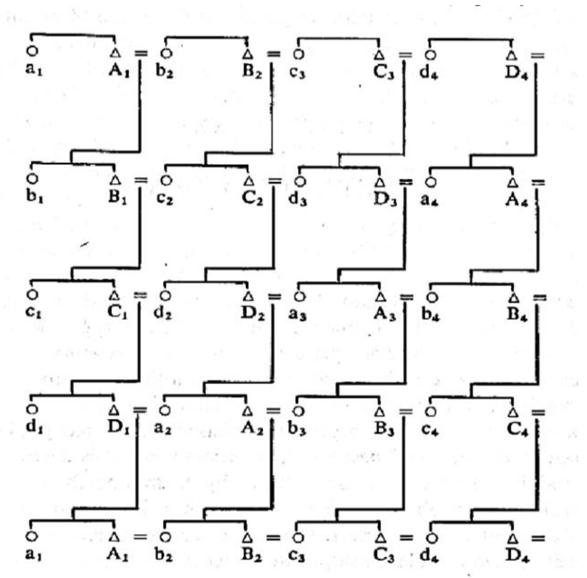
Figure 2.
Illustration of the curve np = 2 showing three histories and connections among those three histories at or above that curve.
Figure 2.
Illustration of the curve np = 2 showing three histories and connections among those three histories at or above that curve.

© 2017 by the author. Licensee MDPI, Basel, Switzerland. This article is an open access article distributed under the terms and conditions of the Creative Commons Attribution (CC BY) license (http://creativecommons.org/licenses/by/4.0/).
Share and Cite
MDPI and ACS Style
Ballonoff, P. Paths of Cultural Systems. Entropy 2018, 20, 8. https://doi.org/10.3390/e20010008
AMA Style
Ballonoff P. Paths of Cultural Systems. Entropy. 2018; 20(1):8. https://doi.org/10.3390/e20010008
Chicago/Turabian StyleBallonoff, Paul. 2018. "Paths of Cultural Systems" Entropy 20, no. 1: 8. https://doi.org/10.3390/e20010008
Note that from the first issue of 2016, this journal uses article numbers instead of page numbers. See further details here.