Detection of Parameter Change in Random Coefficient Integer-Valued Autoregressive Models

Research Institute for Basic Sciences, Jeju National University, Jeju 63243, Korea
Entropy 2018, 20(2), 107; https://doi.org/10.3390/e20020107
Submission received: 5 December 2017
/
Revised: 2 February 2018
/
Accepted: 3 February 2018
/
Published: 6 February 2018
(This article belongs to the Section Statistical Physics)
Abstract
:This paper considers the problem of testing for parameter change in random coefficient integer-valued autoregressive models. To overcome some size distortions of the existing estimate-based cumulative sum (CUSUM) test, we suggest estimating function-based test and residual-based CUSUM test. More specifically, we employ the estimating function of the conditional least squares estimator. Under the regularity conditions and the null hypothesis, we derive their limiting distributions, respectively. Simulation results demonstrate the validity of the proposed tests. A real data analysis is performed on the polio incidence data.
1. Introduction
In recent years, time series of counts are widely observed in real-world applications, for instance, the monthly number of people with a certain disease, the number of transactions per minute of some stock, the number of accidents per a day and so on. Among the existing models for analyzing those data sets, autoregressive moving average (ARMA)-type models based on a thinning operator, referred to as integer-valued ARMA models, are still popular since ARMA-type models provide a convenient way to transfer the classical ARMA recursion to discrete-valued time series (cf. Fokianos [1]). Reviews for these models are given by McKenzie [2], Weiß [3], Scotto et al. [4] and references cited therein.
As is addressed in Kang and Lee [5], integer-valued time series, particularly in epidemiology, often undergo a significant change as a result of changes in the quality of health care and the state of patients’ health. It is well known that such a change can affect the statistical inference undesirably and ignoring a parameter change can lead to a false conclusion. Thus, the change point detection has attracted a lot of attention. In the field of integer-valued time series, Fokianos and Fried [6,7] investigated a testing procedure for the detection of intervention effects in linear and log-linear Poisson autoregressive (AR) models. Szabó [8] proposed the test for a change in several crucial parameters of integer-valued autoregressive (INAR) (p) models. Kang and Lee [5,9] constructed the estimate-based cumulative sum (CUSUM) tests for parameter change in random coefficient integer-valued autoregressive (RCINAR) models and Poisson AR models, respectively. More recently, Pap and Szabó [10] developed change detection methods for INAR(p) processes in general and provided the results available under the alternative hypothesis. Doukhan and Kengne [11] proposed two tests based on the likelihood of the observations in a general class of Poisson AR models. Hudecová et al. [12,13,14,15] studied methods for detecting structural changes in INAR and Poisson AR models incorporating the empirical probability generating function and Kang and Song [16] constructed the score test in Poisson AR models.
This study is concerned with change point problem in RCINAR models. The random coefficient setting reflects that the autoregressive coefficient may vary randomly over time due to environmental factors (cf. Zheng et al. [17], Leonenko et al. [18] and Gomes and Canto e Castro [19]). As aforementioned, Kang and Lee [9] developed the estimate-based CUSUM test in RCINAR models. Here, they constructed the test statistics based on the differences to detect a change in parameter , where denotes the estimator based on . Their test statistic is very intuitive, but it has a drawback in that it produces severe size distortions especially when true parameter lies near the boundary of parameter space. This motivates us to consider alternative methods. In this paper, we propose an estimating function (EF)-based test and residual-based CUSUM test.
The EF-based test is constructed using the partial sum of estimating function and may be referred to as Z-process method as in Negri and Nishiyama [20]. Score test for parameter change is an example of the EF-based test. Indeed, the score test has been studied by several authors. See, for example, Horváth and Parzen [21], Berkes et al. [22], and Song and Kang [23]. Residual-based CUSUM test has been used popularly due to its ease of implementation. Because the residuals can avoid dependence structure in time series observations, it usually produces stable sizes. See, for example, Lee et al. [24], Kulperger and Yu [25], Kang and Lee [5] and so on. In this study, we use the conditional least squares estimator (CLSE) to estimate the RCINAR models. Hence, our EF-based test is proposed using the EF of the CLSE. For residual-based test, we define residual of RCINAR model as the difference between the observation and its conditional expectation, and then construct CUSUM test.
This paper is organized as follows. In Section 2, we review the CLSE for RCINAR models and its asymptotic properties. In Section 3, we present the EF-based test and residual-based CUSUM test and derive their limiting null distributions. In Section 4, we perform a simulation study to see the finite sample performance. In Section 5, we apply our tests to the polio incidence data for illustration. Section 6 concludes the paper. All the proofs for the results in Section 3 are provided in the Appendix.
2. CLSE for RCINAR Models
First, the thinning operator is defined as follows: Let X be an integer-valued random variable and , then the thinning operator “∘” takes the form where is an i.i.d. Bernoulli random sequence with mean that is independent of X (cf. Steutal and Van Harn [26]). With this operator, the RCINAR model is defined by
where is an i.i.d. sequence with range [0, 1), is an i.i.d. sequence with range that is independent of and the counting sequences involved in for are mutually independent and independent of . Note that, conditioned on and , follows a binomial distribution with parameters and . Assume that and . According to Proposition 2.2 of Zheng et al. [17], under the assumptions, the Markov chain has a unique stationary distribution. From now on, we suppose that the distribution of the initial value coincides with this uniquely existing stationary distribution, yielding that the sequence is strictly stationary.
Let , and denote the true value of by . To estimate the unknown parameters, we consider the CLSE. Suppose that from the model are observed. Then, the CLSE is obtained by minimizing the conditional sum of squares
over , and is given by
and
Throughout the paper, we use and to denote and , respectively. The symbol denotes the norm for matrices and vectors and is taken under . The symbols and denote convergence in distribution and convergence in probability, respectively. The almost sure convergence is written as “”.
We define the function by , then can be written in the form . And then, the following result can be established by checking the regularity conditions in Klimko and Nelson [27].
Theorem 1.
We have that converges to almost surely and
where V and W are positive definite matrices defined by
with .
3. Parameter Change Test for RCINAR Models
In this section, we consider the problem of testing the following hypotheses:
To this end, we employ the EF-based test and residual-based CUSUM test.
3.1. EF-Based Test
First, we consider the EF-based test using the partial sum process of the following estimating function:
As the estimate-based test in Kang and Lee [9] is constructed based on the differences , we construct a test statistic using the differences . Noting the fact that , we can see that the differences become . Then, the test statistic is proposed as the maximum value of a function of . To derive its limiting distribution, it is needed to obtain the limiting distribution of for each .
By Taylor’s theorem, we have that for each ,
where is an intermediate point between and and is the integer part of . Here, noting the fact that does not depend on the parameter , we have for all . Thus, we can see that for each ,
It follows from and that for ,
Let , then a.s. by the ergodicity of . The above equation can be rewritten as
Consequently, from and , we can write that
where
In fact, it can be verified that
where is a 2-dimensional standard Brownian bridge (see Lemma A1 in the Appendix). Here, be the function space with respect to the Skorohod topology and the symbol denotes the weak convergence in function space. Here, denotes the inverse of the unique positive definite square root of the positive definite matrix W. Furthermore, and are asymptotically negligible (see Lemmas A2 and A3 in the Appendix, respectively). Hence, combining the above arguments, we obtain our first main result.
Theorem 2.
Under , we have
thus
where is a consistent estimator of W. We reject if is large.
Remark 1.
As a consistent estimator of W, one can consider to use
3.2. Residual-Based CUSUM Test
Instead of the EF-based test, we consider the test statistic based on the residuals, which may be defined as the difference between and its conditional expectation (cf. Freeland and McCabe [28]). For RCINAR models, the residuals are obtained as . Let be the -field generated by . Since forms a sequence of martingale differences, the invariance principle shows that
where . This allows us to construct the residual-based CUSUM test. Here, we replace the residuals with , where and are the CLSE of and , respectively. Using the fact that , we propose the test statistic as follows:
From Lemmas A4 and A5, we can see that
and
respectively. Owing to these and , we have the second main result.
Theorem 3.
Under , we have
We reject if is large.
4. Simulation Results
In this section, we evaluate the performance of our tests and . For the comparison purpose, we additionally perform the estimate-based CUSUM test, , of Kang and Lee [9] given by
where
Kang and Lee [9] showed that under ,
We consider the RCINAR model
where is an i.i.d. sequence of Beta random variables with parameters and is an i.i.d. Poisson sequence with mean . Here, we evaluate , and with sample sizes at the nominal level 0.05: the associated critical values, obtained through Monte Carlo simulations, are 2.408, 1.353 and 2.408, respectively. For each simulation, the first 1000 initial observations are discarded to avoid initialization effects. The empirical sizes and powers are calculated as the proportion of the number of rejections of the null hypothesis based on 1000 repetitions.
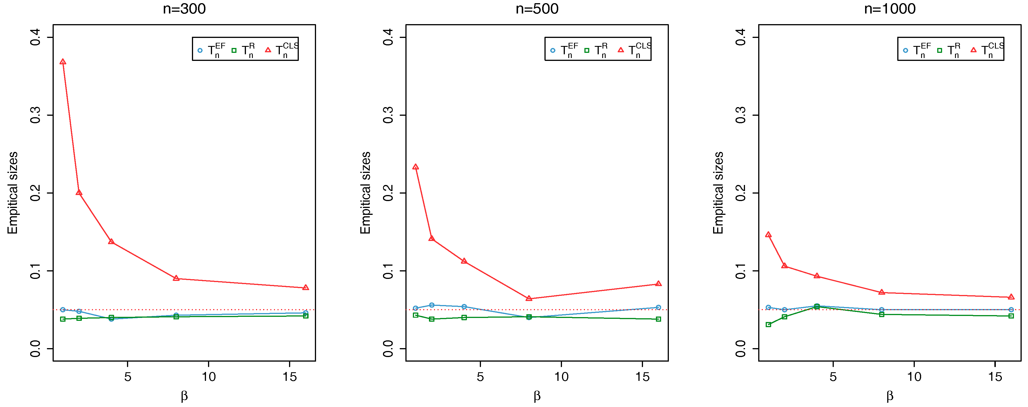
In order to calculate empirical sizes, observations are generated from the model with
for fixed . Since the varies with a and b, we consider the various combinations of to detect the change of the parameters and . Note that tends to 1 as b gets close to 1. The empirical sizes are dotted in Figure 1, where the horizontal dashed lines represent the nominal level 0.05. We can conclude that the empirical sizes are adequate if the empirical sizes are located near the horizontal dashed lines. From the figure, it can be seen that none of and has severe size distortions even for the case that b is close to 1. In contrast, as seen in Kang and Lee [9], shows sever size distortions when b is close to 1. Although not reported here, we could see that the results for other are similar to the case of . Hence, our tests remedy this defect of existing test .
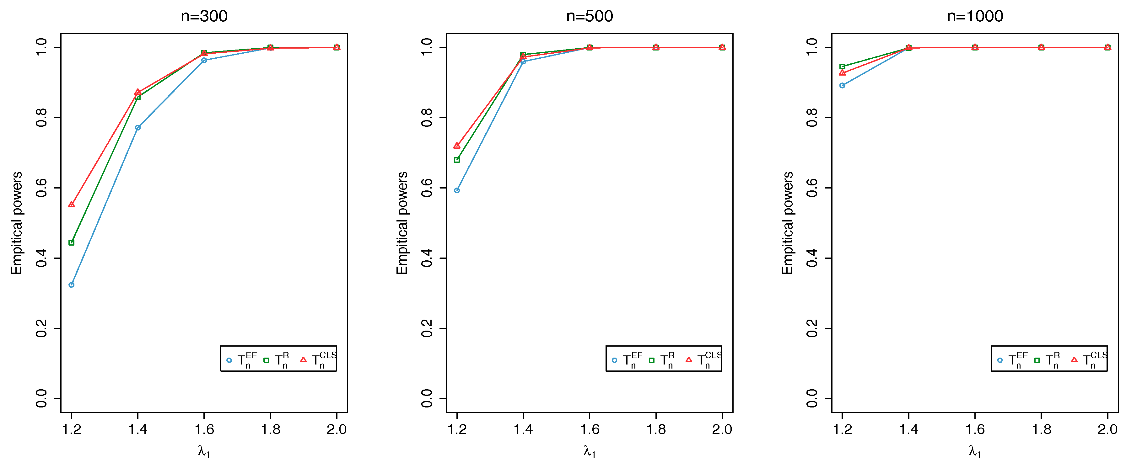
In order to examine the empirical powers, we consider the following alternatives,
In particular, we consider the two cases:
- (i)
- = 1 changes to = 1.2, 1.4, 1.6, 1.8, 2.0 and b = 4 dose not change.
- (ii)
- = 8 changes to = 7, 6 and changes in the same way as in (i).
5. Real Data Analysis
In this section, we apply the proposed tests in Section 3 to analyze the monthly counts of poliomyelitis cases in the US from January 1970 through December 1983, as reported by the Centers for Disease Control and Prevention. The polio incidence data is one of the most famous data sets in the context of time series of counts. This data set has been previously studied by many researchers, such as Zeger [29], Davis et al. [30], Jung and Tremayne [31] and Kang and Lee [5,9]. The data are plotted in Figure 5 and consist of 168 observations. By investigating the sample ACF and by observing the spikes, we fit the RCINAR model to the polio incidence data and examine whether a parameter change exists or not.
In order to test for a change in , and are performed at the nominal level 0.1; the corresponding critical values are 2.054 and 1.212, respectively (cf. the horizontal lines in Figure 6). As a result, we obtain = 2.166 and indicating rejection of the null hypothesis. Since both and have a maximum at (cf. Figure 6), the location of the change can be estimated as November 1972. It is the same result as those of Kang and Lee [5,9].
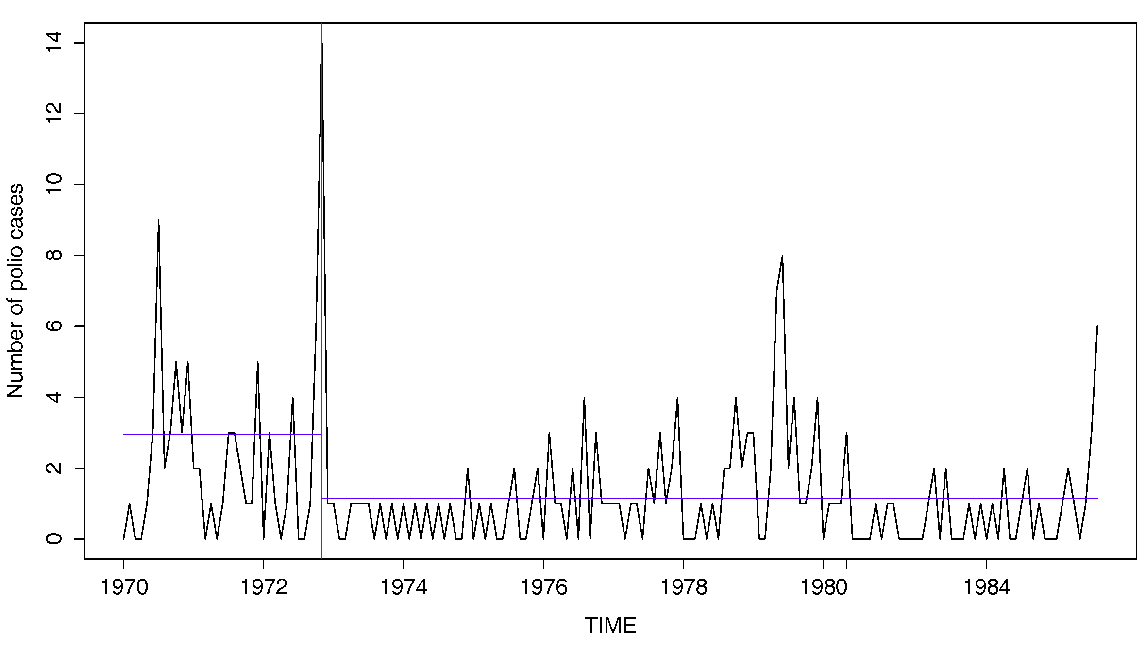
As we have already seen in Kang and Lee [9], it is revealed that the data in the first period, from January 1970 through October 1972, follows RCINAR model with
whereas the data in the second period follows RCINAR model with
Meanwhile, if the change is ignored and the RCINAR(1) model is fitted to the whole observations,
The figures within the parentheses denote the corresponding standard errors.
It can be seen that the estimated parameters in the first period are different from those in the second period. This indicates that ignoring a parameter change can lead to a false result. Furthermore, Figure 7 displays the polio series with the horizontal lines indicating the sample means of the first and second periods, which are 2.95 and 1.15, respectively. It looks quite evident that the series before and after November 1972 have different levels. Overall, the existence of a change is supported in this data.
6. Conclusions
In this study, we constructed an estimating function-based test and residual-based CUSUM test to detect a parameter change in RCINAR models and derived their limiting null distributions. According to simulation results, the proposed tests produce stable sizes even for the case that true parameter lies near the boundary of parameter space and reasonably good powers. Additionally, through a real data analysis, we demonstrated that there exists a parameter change in polio incidence data, which is consistent with previous research. Therefore, our tests can be useful tools in detecting for parameter change.
We anticipate that our tests can extend to other types of integer-valued models. Although we only derived asymptotic null distributions of the proposed tests, the behavior under the alternative, i.e., the consistency of the tests, is also of great interest. Indeed, there are several studies such as Pap and Szabó [10], Hudecová et al. [15] and Doukhan and Kengne [11] dealing with the consistency of each test in time series of counts. As with their studies, we presume that our tests also have the consistency property based on our simulation results (not reported). We leave these issues as a task for our future study.
Acknowledgments
The author is deeply grateful to the anonymous referees for carefully examining the paper and providing valuable comments which improved the paper. The author also thanks Junmo Song for valuable comments and encouragement.
Conflicts of Interest
The author declares no conflict of interest.
Appendix A
In this appendix, we provide proofs for the Theorems 2 and 3 in Section 3.
Lemma A1.
Under ,
Proof of Lemma A1.
Note that . Since is strictly stationary and ergodic, it follows from the functional limit theorem for martingales that
that is,
where is a 2-dimensional standard Brownian motion. Furthermore, by the martingale central limit theorem, we have
This completes the proof. ☐
Lemma A2.
Under ,
Proof of Lemma A2.
Note that
Since , it can be shown that
and
which subsequently yield that
Owing to this and (A1), the lemma is established. ☐
Lemma A3.
Under ,
Proof of Lemma A3.
Due to (A2), we have
together with the facts that and , the lemma is established. ☐
Lemma A4.
Under ,
Proof of Lemma A4.
Note that
Since is ergodic and , the right-hand side of the inequality is . This completes the proof. ☐
Lemma A5.
Under ,
References
- Fokianos, K. Some recent progress in count time series. Statistics 2011, 45, 49–58. [Google Scholar] [CrossRef]
- McKenzie, E. Discrete variate time series. Stochastic processes: Modelling and simulation. In Handbook of Statistics; Shanbhag, D.N., Rao, C.R., Eds.; Elsevier Science: Amsterdam, The Netherlands, 2003; Volume 21, pp. 573–606. ISBN 9780444500137. [Google Scholar]
- Weiß, C.H. Thinning operations for modeling time series of counts a survey. AStA Adv. Stat. Anal. 2008, 92, 319–341. [Google Scholar] [CrossRef]
- Scotto, M.G.; Weiß, C.H.; Gouveia, S. Thinning-based models in the analysis of integer-valued time series: A review. Stat. Model. 2015, 15, 590–618. [Google Scholar] [CrossRef]
- Kang, J.; Lee, S. Parameter change test for Poisson autoregressive models. Scand. J. Stat. 2014, 41, 1136–1152. [Google Scholar] [CrossRef]
- Fokianos, K.; Fried, R. Interventions in INGARCH processes. J. Time Ser. Anal. 2010, 31, 210–225. [Google Scholar] [CrossRef]
- Fokianos, K.; Fried, R. Interventions in log-linear Poisson Autoregression. Stat. Model. 2012, 12, 299–322. [Google Scholar] [CrossRef]
- Szabó, T.T. Test statistics for parameter changes in INAR(p) models and a simulation study. Aust. J. Stat. 2011, 40, 265–280. [Google Scholar] [CrossRef]
- Kang, J.; Lee, S. Parameter change test for random coefficient integer-valued autoregressive processes with application to polio data analysis. J. Time Ser. Anal. 2009, 30, 239–258. [Google Scholar] [CrossRef]
- Pap, G.; Szabó, T.T. Change detection in INAR(p) processes against various alternative hypotheses. Commun. Stat. Theory Methods 2013, 42, 1386–1405. [Google Scholar] [CrossRef]
- Doukhan, P.; Kengne, W. Inference and testing for structural change in general Poisson autoregressive models. Electron. J. Stat. 2015, 9, 1267–1314. [Google Scholar] [CrossRef]
- Hudecová, Š.; Hušková, M.; Meintanis, S.G. Detection of changes in INAR models. In Stochastic Models, Statistics and Their Applications; Steland, A., Rafajlowicz, E., Szajowski, K., Eds.; Springer: New York, NY, USA, 2015; pp. 11–18. [Google Scholar]
- Hudecová, Š.; Hušková, M.; Meintanis, S.G. Tests for time series of counts based on the probability generating function. Statistics 2015, 49, 316–337. [Google Scholar] [CrossRef]
- Hudecová, Š.; Hušková, M.; Meintanis, S.G. Change detection in INARCH time series of counts. In Nonparametric Statistics; Cao, R., Gonzalez Manteiga, W., Romo, J., Eds.; Springer: New York, NY, USA, 2016; pp. 47–58. [Google Scholar]
- Hudecová, Š.; Hušková, M.; Meintanis, S.G. Tests for structural changes in time series of counts. Scand. J. Stat. 2017, 44, 843–865. [Google Scholar] [CrossRef]
- Kang, J.; Song, J. Score test for parameter change in Poisson autoregressive models. Econ. Lett. 2017, 160, 33–37. [Google Scholar]
- Zheng, H.T.; Basawa, I.V.; Datta, S. The first order random coefficient integer-valued autoregressive processes. J. Stat. Plan. Inference 2007, 173, 212–229. [Google Scholar] [CrossRef]
- Leonenko, N.N.; Savani, V.; Zhigljavsky, A.A. Autoregressive negative binomial processes. Ann. ISUP 2007, 51, 25–47. [Google Scholar]
- Gomes, D.; e Castro, L.C. Generalized integer-valued random coefficient for a first order structure autoregressive (RCINAR) process. J. Stat. Plan. Inference 2009, 139, 4088–4097. [Google Scholar] [CrossRef]
- Negri, I.; Nishiyama, Y. Z-process method for change point problems with applications to discretely observed diffusion processes. Stat. Methods Appl. 2017, 26, 231–250. [Google Scholar] [CrossRef]
- Horváth, L.; Parzen, E. Limit theorems for Fisher-score change processes. Lect. Notes Monogr. Ser. 1994, 23, 157–169. [Google Scholar]
- Berkes, I.; Horváth, L.; Kokoszka, P. Testing for parameter constancy in GARCH(p,q) models. Stat. Probab. Lett. 2004, 4, 263–273. [Google Scholar] [CrossRef]
- Song, J.; Kang, J. Parameter change tests for ARMA-GARCH models. Comput. Stat. Data Anal. 2018, 121, 41–56. [Google Scholar] [CrossRef]
- Lee, S.; Tokutsu, Y.; Maekawa, K. The cusum test for parameter change in regression models with ARCH errors. J. Jpn. Stat. Soc. 2004, 34, 173–188. [Google Scholar] [CrossRef]
- Kulperger, R.; Yu, H. High moment partial sum processes of residuals in GARCH models and their applications. Ann. Stat. 2005, 33, 2395–2422. [Google Scholar] [CrossRef]
- Steutal, F.; Van Harn, K. Discrete analogues of self decomposability and stability. Ann. Probab. 1979, 7, 893–899. [Google Scholar]
- Klimko, L.A.; Nelson, P.I. On conditional least squares estimation for stochastic processes. Ann. Stat. 1978, 6, 629–642. [Google Scholar] [CrossRef]
- Freeland, R.K.; McCabe, B.P. Analysis of low count time series data by Poisson autoregression. J. Time Ser. Anal. 2004, 25, 701–722. [Google Scholar] [CrossRef]
- Zeger, S.L. A regression model for time series of counts. Biometrika 1988, 75, 621–629. [Google Scholar] [CrossRef]
- Davis, R.A.; Dunsmuir, W.; Wang, Y. On autocorrelation in a Poisson regression model. Biometrika 2000, 87, 491–505. [Google Scholar] [CrossRef]
- Jung, R.C.; Tremayne, A.R. Useful models for time series of counts or simply wrong ones? AStA Adv. Stat. Anal. 2011, 95, 59–91. [Google Scholar] [CrossRef]
Figure 1.
Plots of empirical powers of , and at nominal level 0.05 when changes to and does not change.
Figure 1.
Plots of empirical powers of , and at nominal level 0.05 when changes to and does not change.
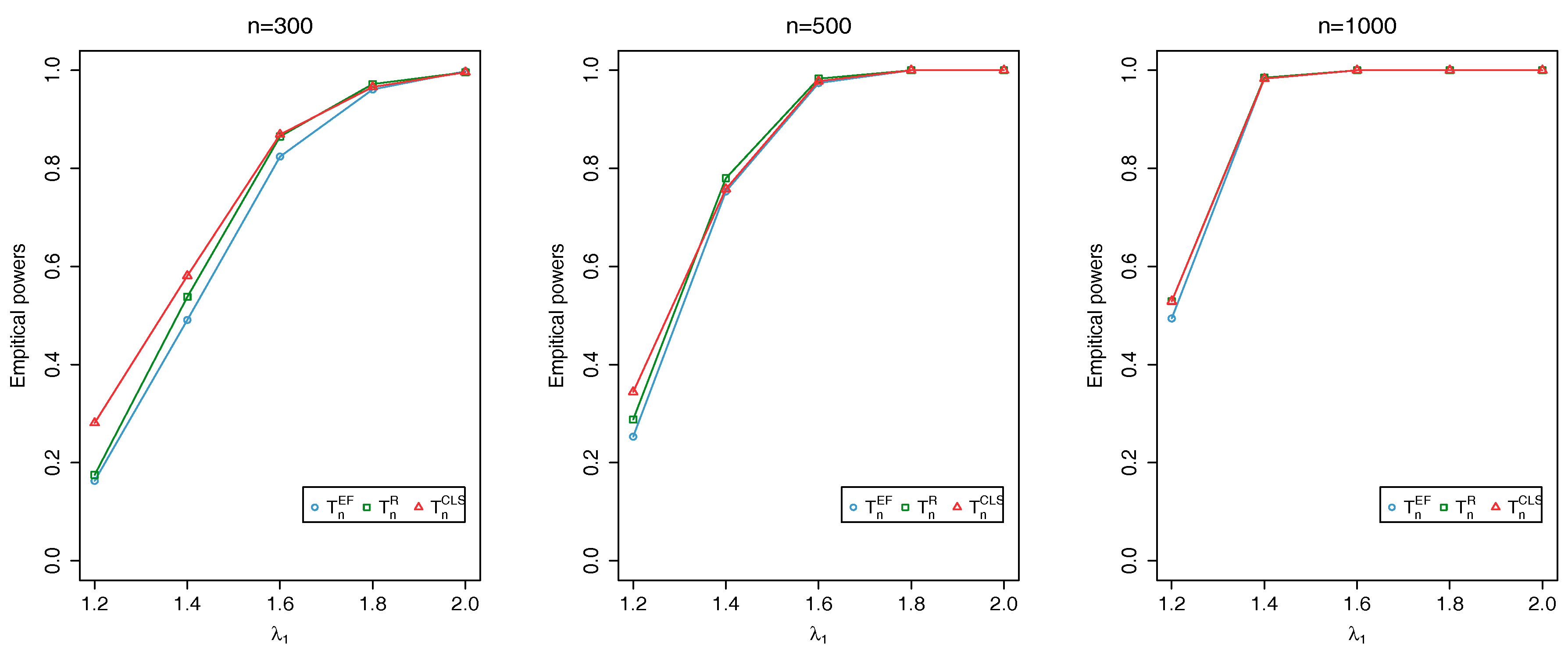
Figure 2.
Plots of empirical sizes of , and at nominal level 0.05.

Figure 3.
Plots of empirical powers of , and at nominal level 0.05 when changes to and changes to .
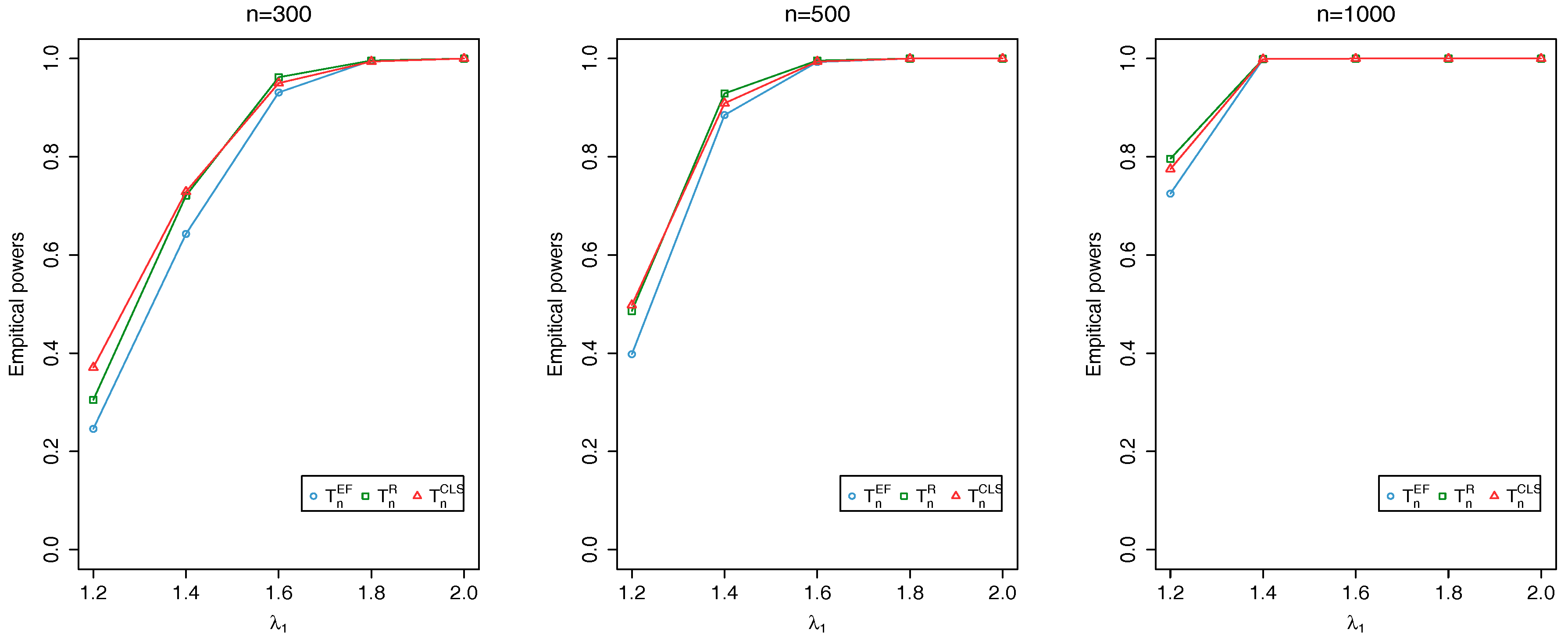
Figure 4.
Plots of empirical powers of , and at nominal level 0.05 when changes to and changes to .

Figure 5.
Plot of the number of polio cases in US from January 1970 to December 1983.
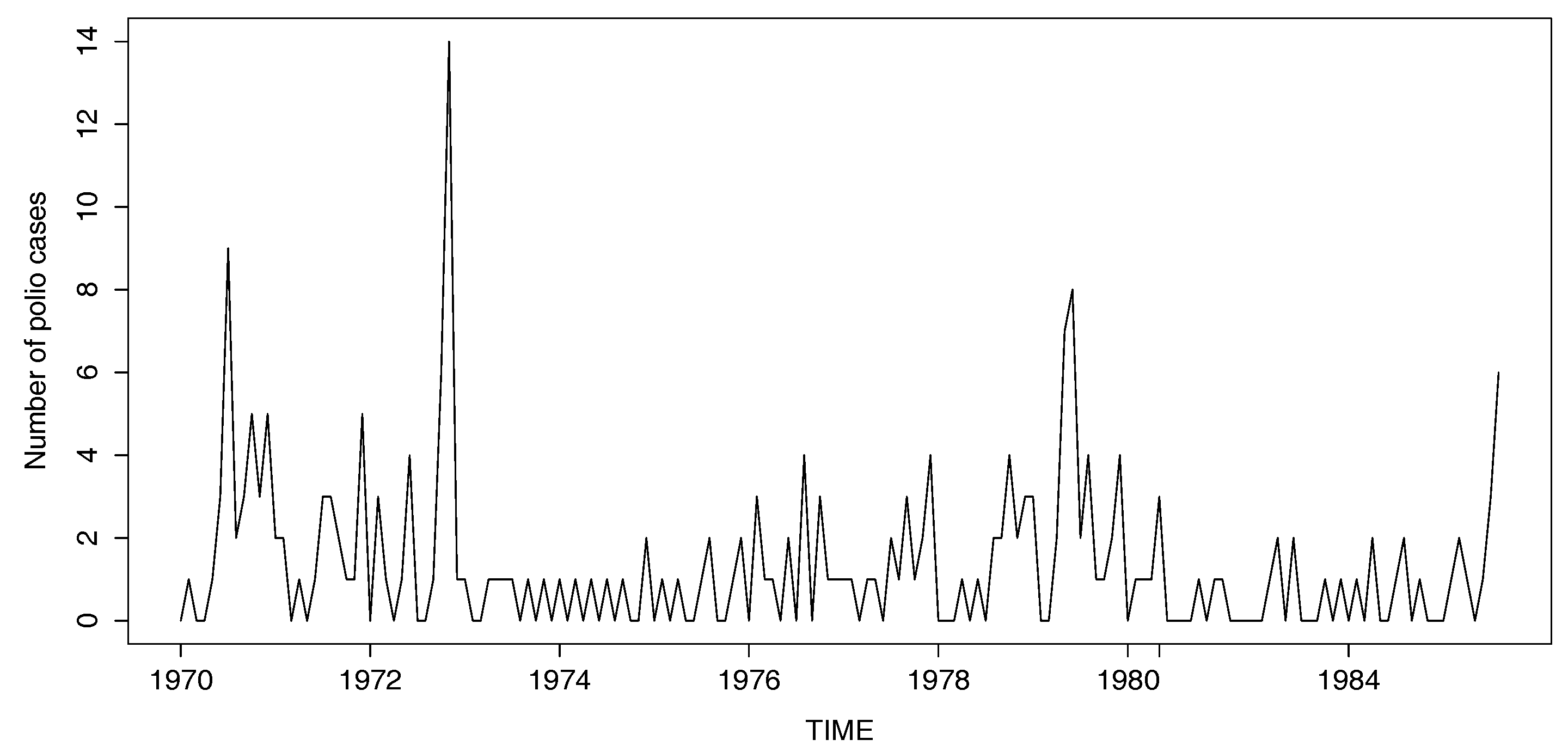
Figure 6.
Plots of (a) and (b) with change at .
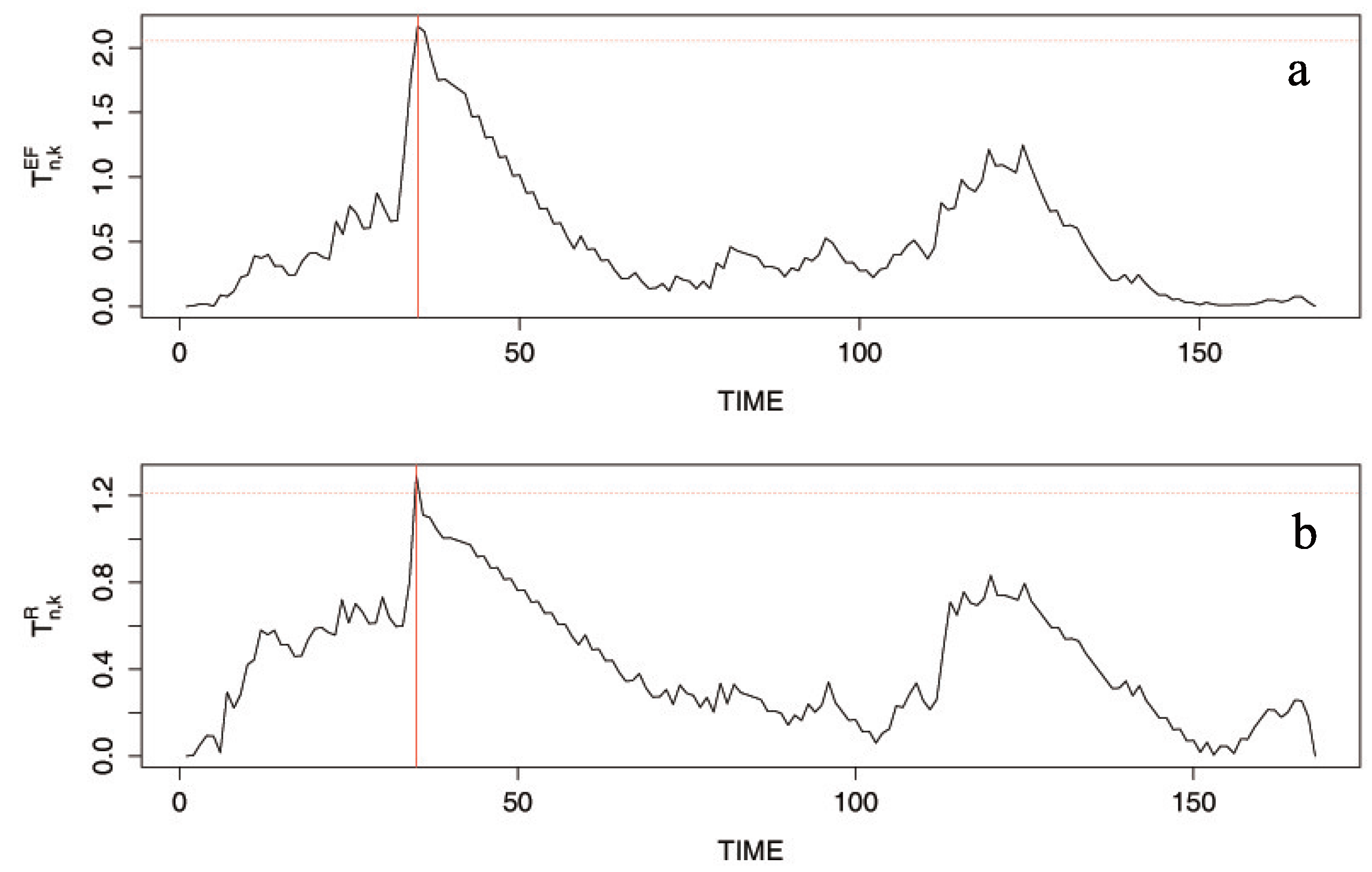
Figure 7.
Plot of the number of polio cases with change in November 1972.
© 2018 by the author. Licensee MDPI, Basel, Switzerland. This article is an open access article distributed under the terms and conditions of the Creative Commons Attribution (CC BY) license (http://creativecommons.org/licenses/by/4.0/).
Share and Cite
MDPI and ACS Style
Kang, J. Detection of Parameter Change in Random Coefficient Integer-Valued Autoregressive Models. Entropy 2018, 20, 107. https://doi.org/10.3390/e20020107
AMA Style
Kang J. Detection of Parameter Change in Random Coefficient Integer-Valued Autoregressive Models. Entropy. 2018; 20(2):107. https://doi.org/10.3390/e20020107
Chicago/Turabian StyleKang, Jiwon. 2018. "Detection of Parameter Change in Random Coefficient Integer-Valued Autoregressive Models" Entropy 20, no. 2: 107. https://doi.org/10.3390/e20020107
Note that from the first issue of 2016, this journal uses article numbers instead of page numbers. See further details here.