Robustness Property of Robust-BD Wald-Type Test for Varying-Dimensional General Linear Models


1
Department of Statistics and Finance, School of Management, University of Science and Technology of China, Hefei 230026, China
2
Department of Statistics, University of Wisconsin-Madison, Madison, WI 53706, USA
*
Author to whom correspondence should be addressed.
Entropy 2018, 20(3), 168; https://doi.org/10.3390/e20030168
Submission received: 12 January 2018
/
Revised: 1 March 2018
/
Accepted: 1 March 2018
/
Published: 5 March 2018
(This article belongs to the Special Issue New Developments in Statistical Information Theory Based on Entropy and Divergence Measures)
Abstract
:An important issue for robust inference is to examine the stability of the asymptotic level and power of the test statistic in the presence of contaminated data. Most existing results are derived in finite-dimensional settings with some particular choices of loss functions. This paper re-examines this issue by allowing for a diverging number of parameters combined with a broader array of robust error measures, called “robust-”, for the class of “general linear models”. Under regularity conditions, we derive the influence function of the robust- parameter estimator and demonstrate that the robust- Wald-type test enjoys the robustness of validity and efficiency asymptotically. Specifically, the asymptotic level of the test is stable under a small amount of contamination of the null hypothesis, whereas the asymptotic power is large enough under a contaminated distribution in a neighborhood of the contiguous alternatives, thus lending supports to the utility of the proposed robust- Wald-type test.
1. Introduction
The class of varying-dimensional “general linear models” [1], including the conventional generalized linear model ( in [2]), is flexible and powerful for modeling a large variety of data and plays an important role in many statistical applications. In the literature, it has been extensively studied that the conventional maximum likelihood estimator for the is nonrobust; for example, see [3,4]. To enhance the resistance to outliers in applications, many efforts have been made to obtain robust estimators. For example, Noh et al. [5] and Künsch et al. [6] developed robust estimator for the , and Stefanski et al. [7], Bianco et al. [8] and Croux et al. [9] studied robust estimation for the logistic regression model with the deviance loss as the error measure.
Besides robust estimation for the , robust inference is another important issue, which, however, receives relatively less attention. Basically, the study of robust testing includes two aspects: (i) establishing the stability of the asymptotic level under small departures from the null hypothesis (i.e., robustness of “validity”); and (ii) demonstrating that the asymptotic power is sufficiently large under small departures from specified alternatives (i.e., robustness of “efficiency”). In the literature, robust inference has been conducted for different models. For example, Heritier et al. [10] studied the robustness properties of the Wald, score and likelihood ratio tests based on M estimators for general parametric models. Cantoni et al. [11] developed a test statistic based on the robust deviance, and conducted robust inference for the using quasi-likelihood as the loss function. A robust Wald-type test for the logistic regression model is studied in [12]. Ronchetti et al. [13] concerned the robustness property for the generalized method of moments estimators. Basu et al. [14] proposed robust tests based on the density power divergence (DPD) measure for the equality of two normal means. Robust tests for parameter change have been studied using the density-based divergence method in [15,16]. However, the aforementioned methods based on the mostly focus on situations where the number of parameters is fixed and the loss function is specific.
Zhang et al. [1] developed robust estimation and testing for the “general linear model” based on a broader array of error measures, namely Bregman divergence, allowing for a diverging number of parameters. The Bregman divergence includes a wide class of error measures as special cases, e.g., the (negative) quasi-likelihood in regression, the deviance loss and exponential loss in machine learning practice, among many other commonly used loss functions. Zhang et al. [1] studied the consistency and asymptotic normality of their proposed robust- parameter estimator and demonstrated the asymptotic distribution of the Wald-type test constructed from robust- estimators. Naturally, it remains an important issue to examine the robustness property of the robust- Wald-type test [1] in the varying-dimensional case, i.e., whether the test still has stable asymptotic level and power, in the presence of contaminated data.
This paper aims to demonstrate the robustness property of the robust- Wald-type test in [1]. Nevertheless, it is a nontrivial task to address this issue. Although the local stability for the Wald-type tests have been established for the M estimators [10], generalized method of moment estimators [13], minimum density power divergence estimator [17] and general M estimators under random censoring [18], their results for finite-dimensional settings are not directly applicable to our situations with a diverging number of parameters. Under certain regularity conditions, we provide rigorous theoretical derivation for robust testing based on the Wald-type test statistic. The essential results are approximations of the asymptotic level and power under contaminated distributions of the data in a small neighborhood of the null and alternative hypotheses, respectively.
- Specifically, we show in Theorem 1 that, if the influence function of the estimator is bounded, then the asymptotic level of the test is also bounded under a small amount of contamination.
- We also demonstrate in Theorem 2 that, if the contamination belongs to a neighborhood of the contiguous alternatives, then the asymptotic power is also stable.
Hence, we contribute to establish the robustness of validity and efficiency for the robust- Wald-type test for the “general linear model” with a diverging number of parameters.
The rest of the paper is organized as follows. Section 2 reviews the Bregman divergence (), robust- estimation and the Wald-type test statistic proposed in [1]. Section 3 derives the influence function of the robust- estimator and studies the robustness properties of the asymptotic level and power of the Wald-type test under a small amount of contamination. Section 4 conducts the simulation studies. The technical conditions and proofs are given in Appendix A. A list of notations and symbols is provided in Appendix B.
We will introduce some necessary notations. In the following, C and c are generic finite constants which may vary from place to place, but do not depend on the sample size n. Denote by the expectation with respect to the underlying distribution K. For a positive integer q, let be a zero vector and be the identity matrix. For a vector , the norm is , norm is and the norm is . For a matrix A, the and Frobenius norms of A are and , respectively, where denotes the largest eigenvalue of a matrix and denotes the trace of a matrix.
2. Review of Robust- Estimation and Inference for “General Linear Models”
This section briefly reviews the robust- estimation and inference methods for the “general linear model” developed in [1]. Let be observations from some underlying distribution with the explanatory variables and Y the response variable. The dimension is allowed to diverge with the sample size n. The “general linear model” is given by
and
where F is a known link function, is the vector of unknown true regression parameters, and is a known function. Note that the conventional generalized linear model () satisfying Equations (1) and (2) assumes that follows a particular distribution in the exponential family. However, our “general linear model” does not require explicit form of distributions of the response. Hence, the “general linear model” includes the as a special case. For notational simplicity, denote and .
Bregman divergence () is a class of error measures, which is introduced in [19] and covers a wide range of loss functions. Specifically, Bregman divergence is defined as a bivariate function,
where is the concave generating q-function. For example, for a constant a corresponds to the quadratic loss . For a binary response variable Y, gives the misclassification loss ; gives Bernoulli deviance loss ; gives the hinge loss for the support vector machine; yields the exponential loss used in AdaBoost [20]. Furthermore, Zhang et al. [21] showed that if
where a is a finite constant such that the integral is well-defined, then is the “classical (negative) quasi-likelihood” function with .
To obtain a robust estimator based on , Zhang et al. [1] developed the robust- loss function
where is a bounded odd function, such as the Huber -function [22], denotes the Pearson residual and is the bias-correction term satisfying
with
Based on robust-, the estimator of proposed in [1] is defined as
where is a known bounded weight function which downweights the high leverage points.
In [11], the “robust quasi-likelihood estimator” of is formulated according to the “robust quasi-likelihood function” defined as
where and , . To describe the intuition of the “robust-”, we use the following diagram from [1], which illustrates the relation among the “robust-”, “classical-”, “robust quasi-likelihood” and “classical (negative) quasi-likelihood”.

For the robust-, assume that
exist finitely up to any order required. For example, for ,
where . Explicit expressions for () can be found in Equation (3.7) of [1]. Then, the estimation equation for is
where the score vector is
with . The consistency and asymptotic normality of have been studied in [1]; see Theorems 1 and 2 therein.
Furthermore, to conduct statistical inference for the “general linear model”, the following hypotheses are considered,
where is a given matrix such that with being a positive-definite matrix, and is a known vector.
To perform the test of Equation (8), Zhang et al. [1] proposed the Wald-type test statistic,
constructed from the robust- estimator in Equation (5), where
The asymptotic distributions of under the null and alternative hypotheses have been developed in [1]; see Theorems 4–6 therein.
On the other hand, the issue on the robustness of , used for possibly contaminated data, remains unknown. Section 3 of this paper will address this issue with detailed derivations.
3. Robustness Properties of in Equation (9)
This section derives the influence function of the robust- Wald-type test and studies the influence of a small amount of contamination on the asymptotic level and power of the test. The proofs of the theoretical results are given in Appendix A.
Denote by the true distribution of following the “general linear model” characterized by Equations (1) and (2). To facilitate the discussion of robustness properties, we consider the -contamination,
where J is an arbitrary distribution and is a constant. Then, is a contaminated distribution of with the amount of contamination converging to 0 at rate . Denote by the empirical distribution of .
For a generic distribution K of , define
where and are defined in Equations (4) and (7), respectively. It’s worth noting that the solution to may not be unique, i.e., may contain more than one element. We then define a functional for the estimator of as follows,
From the result of Lemma A1 in Appendix A, is the unique local minimizer of in the -neighborhood of . Particularly, . Similarly, from Lemma A2 in Appendix A, is the unique local minimizer of which satisfies .
From [23] (Equation (2.1.6) on pp. 84), the influence function of at is defined as
where is the probability measure which puts mass 1 at the point . Since the dimension of diverges with n, its influence function is defined for each fixed n. From Lemma A8 in Appendix A, under certain regularity conditions, the influence function exists and has the following expression:
where . The form of the influence function for diverging in Equation(13) coincides with that in [23,24] for fixed .
In our theoretical derivations, approximations of the asymptotic level and power of will involve the following matrices:
3.1. Asymptotic Level of under Contamination
We now investigate the asymptotic level of the Wald-type test under the -contamination.
Theorem 1.
Assume Conditions A0–A9 and B4 in Appendix A. Suppose as , . Denote by the level of when the underlying distribution is in Equation (10) and by the nominal level. Under in Equation (8), it follows that
where
, is the cumulative distribution function of a distribution, and is the quantile of the central distribution.
Theorem 1 indicates that if the influence function for is bounded, then the asymptotic level of under the -contamination is also bounded and close to the nominal level when is sufficiently small. As a comparison, the robustness property in [10] of the Wald-type test is studied based on M-estimator for general parametric models with a fixed dimension . They assumed certain conditions that guarantee Fréchet differentiability which further implies the existence of the influence function and the asymptotic normality of the corresponding estimator. However, in the set-ups of our paper, it’s difficult to check those conditions, due to the use of Bregman divergence and the diverging dimension . Hence, the assumptions we make in Theorem 1 are different from those in [10], and are comparatively mild and easy to check. Moreover, the result of Theorem 1 cannot be easily derived from that of [10].
In Theorem 1, is allowed to diverge with , which is slower than that in [1] with . Theoretically, the assumption is required to obtain the asymptotic distribution of in [1]. Furthermore, to derive the limit distribution of under the -contamination, assumption is needed (see Lemma A7 in Appendix A). Hence, the reason that our assumption is stronger than that in [1] is the consideration of the -contamination of the data. Practically, due to the advancement of technology and different forms of data gathering, large dimension becomes a common characteristic and hence the varying-dimensional model has a wide range of applications, e.g., brain imaging data, financial data, web term-document data and gene expression data. Even some of the classical settings, e.g., the Framingham heart study with and , can be viewed as varying-dimensional cases.
As an illustration, we apply the general result of Theorem 1 to the special case of a point mass contamination.
Corollary 1.
In Corollary 1, conditions and are needed to guarantee the boundedness of the score function in Equation (7). Particularly, the function downweights the high leverage points and can be chosen as, e.g., . The condition is needed to bound Equation (6), and is satisfied in many situations.
- For example, for the linear model with , and , where a and are constants, we observe .
- Another example is the logistic regression model with binary response and (corresponding to Bernoulli deviance loss), , . In this case, since . Likewise, if (for the exponential loss), then .
Furthermore, the bound on is useful to control deviations in the Y-space, which ensures the stability of the robust- test if Y is arbitrarily contaminated.
Concerning the dimensionality , Corollary 1 reveals the following implications. If is fixed, then the asymptotic level of under the -contamination is uniformly bounded for all , which implies the robustness of validity of the test. This result coincides with that in Proposition 5 of [10]. When diverges, the asymptotic level is still stable if the point contamination satisfies , where is an arbitrary constant. Although this condition may not be the weakest, it still covers a wide range of point mass contaminations.
3.2. Asymptotic Power of under Contamination
Now, we will study the asymptotic power of under a sequence of contiguous alternatives of the form
where is fixed.
Theorem 2.
Assume Conditions – and in Appendix A. Suppose as , . Denote by the power of when the underlying distribution is in Equation (10) and by the nominal power. Under in Equation (14), it follows that
where
with , and and being defined in Theorem 1.
The result for the asymptotic power is similar in spirit to that for the level. From Theorem 2, if the influence function is bounded, the asymptotic power is also bounded from below and close to the nominal power under a small amount of contamination. This means that the robust- Wald-type test enjoys the robustness of efficiency. In addition, the property of the asymptotic power can be obtained for a point mass contamination.
Corollary 2.
4. Simulation
Regarding the practical utility of , numerical studies concerning the empirical level and power of under a fixed amount of contamination have been conducted in Section 6 of [1]. To support the theoretical results in our paper, we conduct new simulations to check the robustness of validity and efficiency of . Specifically, we will examine the empirical level and power of the test statistic as varies.
The robust- estimation utilizes the Huber -function with and the weight function . Comparisons are made with the classical non-robust counterparts corresponding to using and . For each situation below, we set and conduct 400 replications.
4.1. Overdispersed Poisson Responses
Overdispersed Poisson counts Y, satisfying , are generated via a negative Binomial distribution. Let and , where denotes the floor function. Generate by . The log link function is considered and the (negative) quasi-likelihood is utilized as the BD, generated by the q-function in Equation (3) with . The estimator and test statistic are calculated by assuming Y follows Poisson distribution.
The data are contaminated by and for , with the number of contaminated data points, where is the modulo operation “a modulo b” and . Then, the proportion of contaminated data, , is equal to as in Equation (10), which implies .
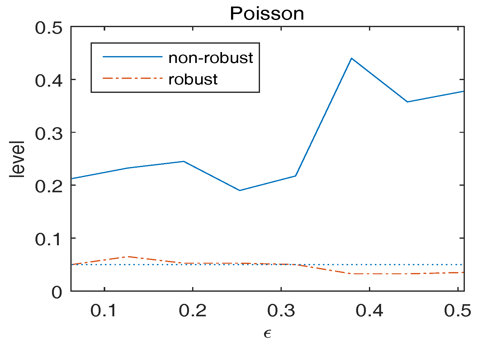
Consider the null hypothesis with . Figure 1 plots the empirical level of versus . We observe that the asymptotic nominal level 0.05 is approximately retained by the robust Wald-type test. On the other hand, under contaminations, the non-robust Wald-type test breaks in level, showing high sensitivity to the presence of outliers.
To assess the stability of the power of the test, we generate the original data from the true model, but with the true parameter replaced by with and a vector of ones. Figure 2 plots the empirical rejection rates of the null model, which implies that the robust Wald-type test has sufficiently large power to detect the alternative hypothesis. In addition, the power of the robust method is generally larger than that of the non-robust method.
4.2. Bernoulli Responses
We generate data with two classes from the model, , where . Let , and . The null hypothesis is . Both the deviance loss and the exponential loss are employed as the BD. We contaminate the data by setting and for with . To investigate the robustness of validity of , we plot the observed level versus in Figure 3. We find that the level of the non-robust method diverges fast as increases. It’s also clear that the empirical level of the robust method is close to the nominal level when is small and increases slightly with , which coincides with our results in Theorem 1.
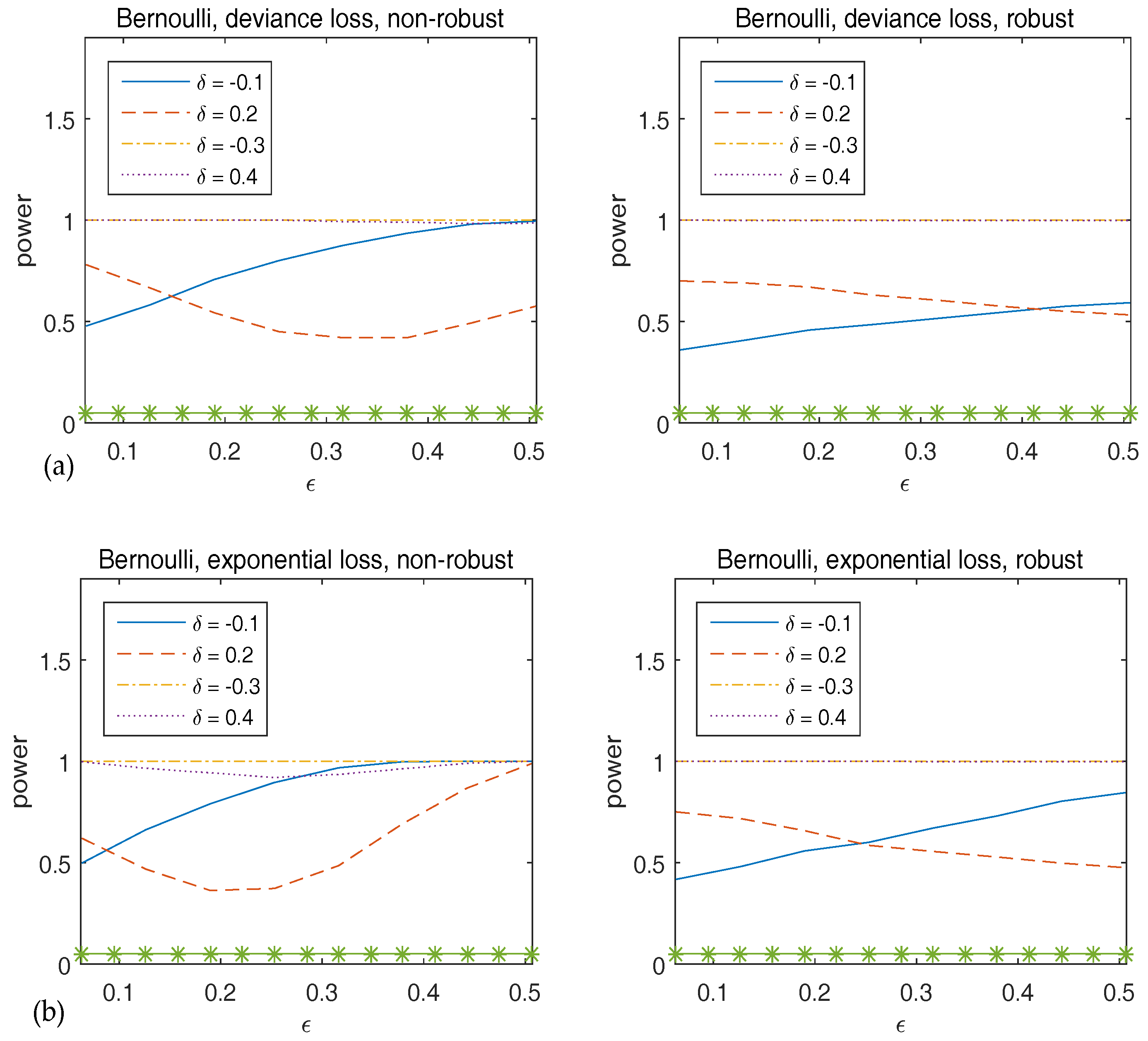
To assess the stability of the power of , we generate the original data from the true model, but with the true parameter replaced by with and a vector of ones. Figure 4 plots the power of the Wald-type test versus , which implies that the robust method has sufficiently large power, and hence supports the theoretical results in Theorem 2.
Acknowledgments
We thank the two referees for insightful comments and suggestions. Chunming Zhang’s research is supported by the U.S. NSF Grants DMS–1712418, DMS–1521761, the Wisconsin Alumni Research Foundation and the National Natural Science Foundation of China, grants 11690014. Xiao Guo’s research is supported by the Fundamental Research Funds for the Central Universities and the National Natural Science Foundation of China, grants 11601500, 11671374 and 11771418.
Author Contributions
Chunming Zhang conceived and designed the experiments; Xiao Guo performed the experiments; Xiao Guo analyzed the data; Chunming Zhang contributed to analysis tools; Chunming Zhang and Xiao Guo wrote the paper.
Conflicts of Interest
The authors declare no conflicts of interest.
Appendix A. Conditions and Proofs of Main Results
We first introduce some necessary notations used in the proof.
Notations.
For arbitrary distributions K and of , define
Therefore, , , and . For notational simplicity, let and .
Define the following matrices,
The following conditions are needed in the proof, which are adopted from [1].
Condition A.
- A0.
- .
- A1.
- is a bounded function. Assume that is a bounded, odd function, and twice differentiable, such that , , , and are bounded; , is continuous.
- A2.
- is continuous, and . is continuous.
- A3.
- is monotone and a bijection, is continuous, and .
- A4.
- almost surely if the underlying distribution is .
- A5.
- exists and is nonsingular.
- A6.
- There is a large enough open subset of which contains , such that is bounded for all in the subset and all such that , where is a large enough constant.
- A7.
- is positive definite, with eigenvalues uniformly bounded away from 0.
- A8.
- is positive definite, with eigenvalues uniformly bounded away from 0.
- A9.
- is bounded away from ∞.
Condition B.
- B4.
- almost surely if the underlying distribution is J.
The following Lemmas A1–A9 are needed to prove the main theoretical results in this paper.
Lemma A1 ().
Proof.
We follow the idea of the proof in [25]. Let and . First, we show that there exists a sufficiently large constant C such that, for large n, we have
To show Equation (A1), consider
where .
By Taylor expansion,
where
for located between and . Hence
since and . For in Equation (A2),
where . Meanwhile, we have
where and . Thus,
For in Equation (A2), we observe that
We can choose some large C such that , and are all dominated by the first term of in Equation (A3), which is positive by the eigenvalue assumption. This implies Equation (A1). Therefore, there exists a local minimizer of in the neighborhood of , and denote this minimizer by .
Next, we show that the local minimizer of is unique in the neighborhood of . For all such that ,
and hence,
Therefore,
We know that the minimum eigenvalues of are uniformly bounded away from 0,
Hence, for n large enough, is positive definite for all such that . Therefore, there exists a unique minimizer of in the neighborhood of which covers . From
we know . From the definition of , it’s easy to see that is unique. ☐
Lemma A2 ().
Proof.
Let and . To show the existence of the estimator, it suffices to show that for any given , there exists a sufficiently large constant such that, for large n we have
This implies that with probability at least , there exists a local minimizer of in the ball . To show Equation (A4), consider
where .
By Taylor expansion,
where
for located between and .
Since , the large open set considered in Condition contains when n is large enough, say where N is a positive constant. Therefore, for any fixed , there exists a bounded open subset of containing such that for all in this set, which is integrable with respect to , where C is a positive constant. Thus, for ,
Hence,
Thus,
For in Equation (A5), we observe that
We will show that the minimum eigenvalue of is uniformly bounded away from 0. . Note
Since the eigenvalues of are uniformly bounded away from 0, so are those of and .
We can choose some large such that and are both dominated by the first term of in Equation (A7), which is positive by the eigenvalue assumption. This implies Equation (A4).
Next we show the uniqueness of . For all such that ,
We know that the minimum eigenvalues of are uniformly bounded away from 0. Following the proof of Lemma A1, we have and . It’s easy to see .
Hence, for n large enough, is positive definite with high probability for all such that . Therefore, there exists a unique minimizer of in the neighborhood of which covers . ☐
Lemma A3 ().
Proof.
Taylor’s expansion yields
where lies between and . Below, we will show
First, . Following the proof of in Lemma A1, . Since , we have .
Therefore, which completes the proof. ☐
Lemma A4 (asymptotic normality of ).
Assume Conditions A0–A8 and B4. If as and the distribution of is , then
where , is any given matrix such that , with being a positive-definite matrix, is a fixed integer.
Proof.
We will first show that
From , Taylor’s expansion yields
where lies between and . Below, we will show
Similar arguments for the proof of of Lemma A2, we have .
Second, a similar proof used for in Equation (A5) gives
Third, by Equation (A9) and , we see that
where . From the proof of Lemma A2, the eigenvalues of are uniformly bounded away from 0 and we complete the proof of Equation (A8).
Following the proof for the bounded eigenvalues of in Lemma A2, we can show that the eigenvalues of are uniformly bounded away from 0. Hence, the eigenvalues of are uniformly bounded away from 0, as are the eigenvalues of . From Equation (A8), we see that
To show , we apply the Lindeberg-Feller central limit theorem in [26]. Specifically, we check (I) ; (II) for some . Condition (I) is straightforward since . To check condition (II), we can show that . This yields . Hence
Thus, we complete the proof. ☐
Lemma A5 (asymptotic covariance matrices and ).
Assume Conditions A0–A9 and B4. If as , then
where , is any given matrix such that , with being a positive-definite matrix, and is a fixed integer.
Proof.
Note that
Since , it suffices to prove that .
First, we prove . Note that
We know that and . Thus, .
Second, we show . It is easy to see that
where and . We observe that .
Third, we show . Note , where , and . Under Conditions and , it is straightforward to see that , and . Since , we conclude , and similarly and . Hence, .
Thus, we can conclude that and that the eigenvalues of and are uniformly bounded away from 0 and ∞. Consequently, and proof is finished. ☐
Lemma A6 (asymptotic covariance matrices and ).
Assume Conditions A0–A9 and B4. If and the distribution of is , then
where is any given matrix such that , with being a positive-definite matrix, and is a fixed integer.
Proof.
Note that . Since , it suffices to prove that .
Following the proof of Proposition 1 in [1], we can show that and .
To show , note , where , and . Following the proof in Lemma A2, it is straightforward to verify that , . In addition, .
Since , we conclude , and similarly and . Hence, .
Thus, we can conclude that and the eigenvalues of are uniformly bounded away from 0 and ∞ with probability tending to 1. Noting that . ☐
Lemma A7 (asymptotic distribution of test statistic).
Assume Conditions A0–A9 and B4. If and the distribution of is , then
where is any given matrix such that , with being a positive-definite matrix, and is a fixed integer.
Proof.
Note that
For term I, we obtain from Lemma A4 that From Lemma A6, we get Thus, by Slutsky theorem,
For term , we see from Lemma A6 that
Since
Thus,
Lemma A8 (Influence Function IF).
Assume Conditions A1–A8 and B4. For any fixed sample size n,
where and is a positive constant such that with a sufficiently small constant. In addition, uniformly for all n and such that with a sufficiently small constant.
Proof.
We follow the proof of Theorem 5.1 in [27]. Note
where .
It suffices to prove that for any sequence such that , we have
Following similar proofs in Lemma A1, we can show that for sufficiently small,
Next we will show that the eigenvalues of are bounded away from 0.
First,
Similarly, and . Since the eigenvalues of are bounded away from zero, , and could be sufficiently small, we conclude that for when c is sufficiently small, the eigenvalues of are uniformly bounded away from 0.
Define . Following similar arguments for (A6) in Lemma A2, for j large enough, . We will only consider j large enough below. The two term Taylor expansion yields
where lies between and .
Next, we will show that as for any fixed n. Since ,
and also,
This completes the proof. ☐
Lemma A9.
Assume Conditions A1–A8 and B4 and . Let be the cumulative distribution function of distribution with δ the noncentrality parameter. Denote . Let . Then, for any fixed , under and under .
Proof.
Since , we have
To complete the proof, we only need to show that and () are bounded as for all . Note that
where is the Gamma function, and is the lower incomplete gamma function which satisfies Therefore,
Since
we have
From the results of Lemma A3, that is bounded as for all under both and , so are (). Now, we consider the derivatives of ,
To complete the proof, we only need to show that () are bounded as for all , and is bounded under and as for all . The result for is straightforward from Lemma A3.
First, for the first order derivative of ,
Since , and
we conclude that is uniformly bounded for all as .
Second, for the second order derivative of ,
with
Therefore, . In addition,
Therefore, for all .
Finally, for the third order derivative of ,
Note:
where
Hence, which implies that for all . In addition,
Hence, . Therefore, for all . Hence, we complete the proof. ☐
Proof of Theorem 1.
We follow the idea of the proof in [10]. Lemma A7 implies that the Wald-type test statistic is asymptotically noncentral with noncentrality parameter . Therefore, where as for any fixed . Let . Then, for close to 0, we have
where . Note that under
From Lemma A8, under
Thus,
Since from Lemma A8, is uniformly bounded, we have
From Equation (A17)
since from Lemma A9. We complete the proof. ☐
Proof of Corollary 1.
For Part , following the proof of Theorem 1, for any fixed ,
where . From the assumption that and , we know . Following the proof of Lemma A9, . We finished the proof of part .
Part is straightforward by applying Theorem 1 with . ☐
Proof of Theorem 2.
Lemma A7 implies that
From Lemmas A5 and A6,
Then, is asymptotically with under . Therefore, , where as for any fixed . Let . Then, for close to 0, we have
where . Note that under , Then,
From Lemma A8,
and hence,
Since under by Lemma A9, we have as .
Since from Lemma A8, is uniformly bounded,
From Equation (A18), we complete the proof. ☐
Proof of Corollary 2.
The proof is similar to that for Corollary 1, using the results in Theorem 2. ☐
Appendix B. List of Notations and Symbols
- : dimensional vector in in Equation (14)
- : link function
- G: bias-correction term in “robust-”
- : limit of , i.e.,
- :
- : influence function
- J: an arbitrary distribution in the contamination of Equation (10)
- : true parametric distribution of
- : , -contamination in Equation (10)
- : empirical distribution of
- : expectation of robust- in Equation (11)
- : conditional mean of Y given in Equation (1)
- n: sample size
- : dimension of
- : ith order derivative of robust-
- : generating q-function of
- : vector, a functional of estimator in Equation (12)
- :
- : conditional variance of Y given in Equation (2)
- : Wald-type test statistic in Equation (9)
- : weight function
- : explanatory variables
- Y: response variable
- : level of the test
- : power of the test
- : true regression parameter
- : probability measure which puts mass 1 at the point
- : amount of contamination in Equation (10), positive constant
- : score vector in Equation (7)
- :
- : robust- in Equation (4)
References
- Zhang, C.M.; Guo, X.; Cheng, C.; Zhang, Z.J. Robust-BD estimation and inference for varying-dimensional general linear models. Stat. Sin. 2012, 24, 653–673. [Google Scholar] [CrossRef]
- McCullagh, P.; Nelder, J.A. Generalized Linear Models, 2nd ed.; Chapman & Hall: London, UK, 1989. [Google Scholar]
- Morgenthaler, S. Least-absolute-deviations fits for generalized linear models. Biometrika 1992, 79, 747–754. [Google Scholar] [CrossRef]
- Ruckstuhl, A.F.; Welsh, A.H. Robust fitting of the binomial model. Ann. Stat. 2001, 29, 1117–1136. [Google Scholar]
- Noh, M.; Lee, Y. Robust modeling for inference from generalized linear model classes. J. Am. Stat. Assoc. 2007, 102, 1059–1072. [Google Scholar] [CrossRef]
- Künsch, H.R.; Stefanski, L.A.; Carroll, R.J. Conditionally unbiased bounded-influence estimation in general regression models, with applications to generalized linear models. J. Am. Stat. Assoc. 1989, 84, 460–466. [Google Scholar]
- Stefanski, L.A.; Carroll, R.J.; Ruppert, D. Optimally bounded score functions for generalized linear models with applications to logistic regression. Biometrika 1986, 73, 413–424. [Google Scholar] [CrossRef]
- Bianco, A.M.; Yohai, V.J. Robust estimation in the logistic regression model. In Robust Statistics, Data Analysis, and Computer Intensive Methods; Springer: New York, NY, USA, 1996; pp. 17–34. [Google Scholar]
- Croux, C.; Haesbroeck, G. Implementing the Bianco and Yohai estimator for logistic regression. Comput. Stat. Data Anal. 2003, 44, 273–295. [Google Scholar] [CrossRef]
- Heritier, S.; Ronchetti, E. Robust bounded-influence tests in general parametric models. J. Am. Stat. Assoc. 1994, 89, 897–904. [Google Scholar] [CrossRef]
- Cantoni, E.; Ronchetti, E. Robust inference for generalized linear models. J. Am. Stat. Assoc. 2001, 96, 1022–1030. [Google Scholar] [CrossRef]
- Bianco, A.M.; Martínez, E. Robust testing in the logistic regression model. Comput. Stat. Data Anal. 2009, 53, 4095–4105. [Google Scholar] [CrossRef]
- Ronchetti, E.; Trojani, F. Robust inference with GMM estimators. J. Econom. 2001, 101, 37–69. [Google Scholar] [CrossRef]
- Basu, A.; Mandal, N.; Martin, N.; Pardo, L. Robust tests for the equality of two normal means based on the density power divergence. Metrika 2015, 78, 611–634. [Google Scholar] [CrossRef] [Green Version]
- Lee, S.; Na, O. Test for parameter change based on the estimator minimizing density-based divergence measures. Ann. Inst. Stat. Math. 2005, 57, 553–573. [Google Scholar] [CrossRef]
- Kang, J.; Song, J. Robust parameter change test for Poisson autoregressive models. Stat. Probab. Lett. 2015, 104, 14–21. [Google Scholar] [CrossRef]
- Basu, A.; Ghosh, A.; Martin, N.; Pardo, L. Robust Wald-type tests for non-homogeneous observations based on minimum density power divergence estimator. ArXiv Pre-print, 2017; arXiv:1707.02333. [Google Scholar]
- Ghosh, A.; Basu, A.; Pardo, L. Robust Wald-type tests under random censoring. ArXiv, 2017; arXiv:1708.09695. [Google Scholar]
- Brègman, L.M. A relaxation method of finding a common point of convex sets and its application to the solution of problems in convex programming. U.S.S.R. Comput. Math. Math. Phys. 1967, 7, 620–631. [Google Scholar] [CrossRef]
- Hastie, T.; Tibshirani, R.; Friedman, J. The Elements of Statistical Learning; Springer: Berlin, Germany, 2001. [Google Scholar]
- Zhang, C.M.; Jiang, Y.; Shang, Z. New aspects of Bregman divergence in regression and classification with parametric and nonparametric estimation. Can. J. Stat. 2009, 37, 119–139. [Google Scholar] [CrossRef]
- Huber, P. Robust estimation of a location parameter. Ann. Math. Statist. 1964, 35, 73–101. [Google Scholar] [CrossRef]
- Hampel, F.R.; Ronchetti, E.M.; Roussecuw, P.J.; Stahel, W.A. Robust Statistics: The Application Based on Influence Function; John Wiley: New York, NY, USA, 1986. [Google Scholar]
- Hampel, F.R. The influence curve and its role in robust estimation. J. Am. Stat. Assoc. 1974, 69, 383–393. [Google Scholar] [CrossRef]
- Fan, J.; Peng, H. Nonconcave penalized likelihood with a diverging number of parameters. Ann. Stat. 2004, 32, 928–961. [Google Scholar]
- Van der Vaart, A.W. Asymptotic Statistics; Cambridge University Press: Cambridge, UK, 1998. [Google Scholar]
- Clarke, B.R. Uniqueness and Fréchet differentiability of functional solutions to maximum likelihood type equations. Ann. Stat. 1983, 11, 1196–1205. [Google Scholar] [CrossRef]
Figure 1.
Observed level of versus for overdispersed Poisson responses. The dotted line indicates the 5% significance level.
Figure 1.
Observed level of versus for overdispersed Poisson responses. The dotted line indicates the 5% significance level.

Figure 2.
Observed power of versus for overdispersed Poisson responses. The statistics in the left panel correspond to non-robust method and those in the right panel are for robust method. The asterisk line indicates the 5% significance level.
Figure 2.
Observed power of versus for overdispersed Poisson responses. The statistics in the left panel correspond to non-robust method and those in the right panel are for robust method. The asterisk line indicates the 5% significance level.
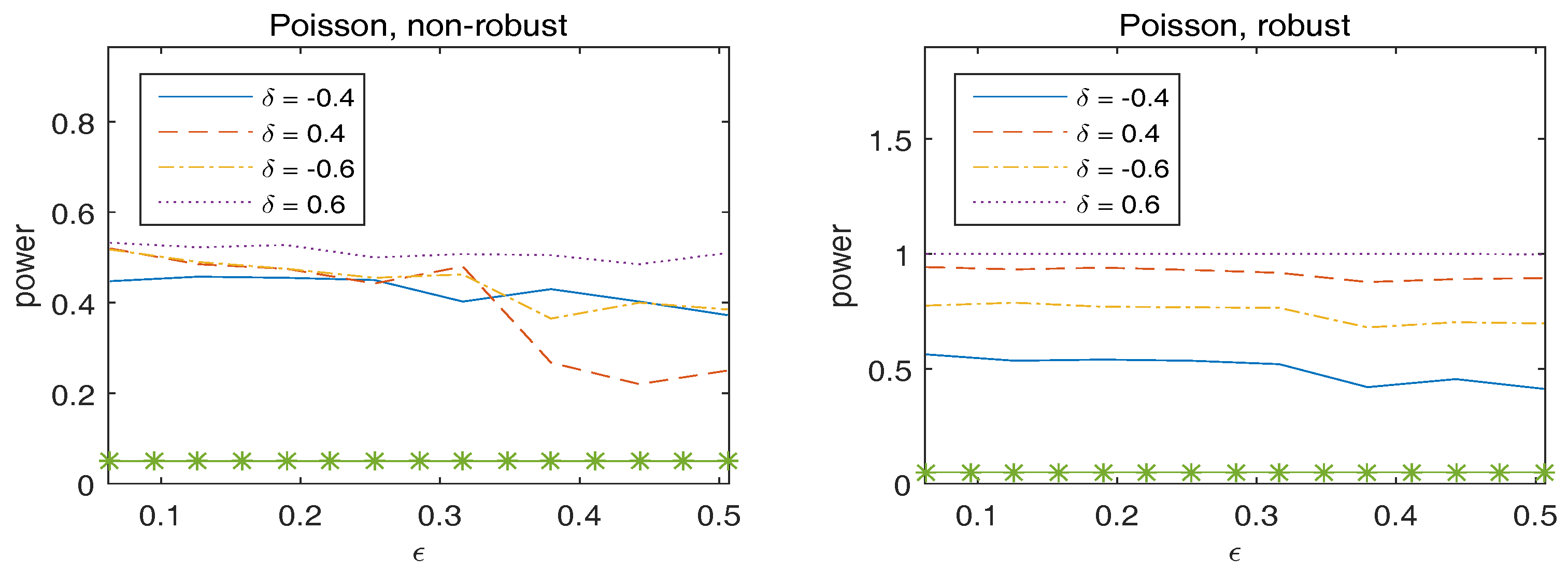
Figure 3.
Observed level of versus for Bernoulli responses. The statistics in (a) use deviance loss and those in (b) use exponential loss. The dotted line indicates the 5% significancelevel.
Figure 3.
Observed level of versus for Bernoulli responses. The statistics in (a) use deviance loss and those in (b) use exponential loss. The dotted line indicates the 5% significancelevel.
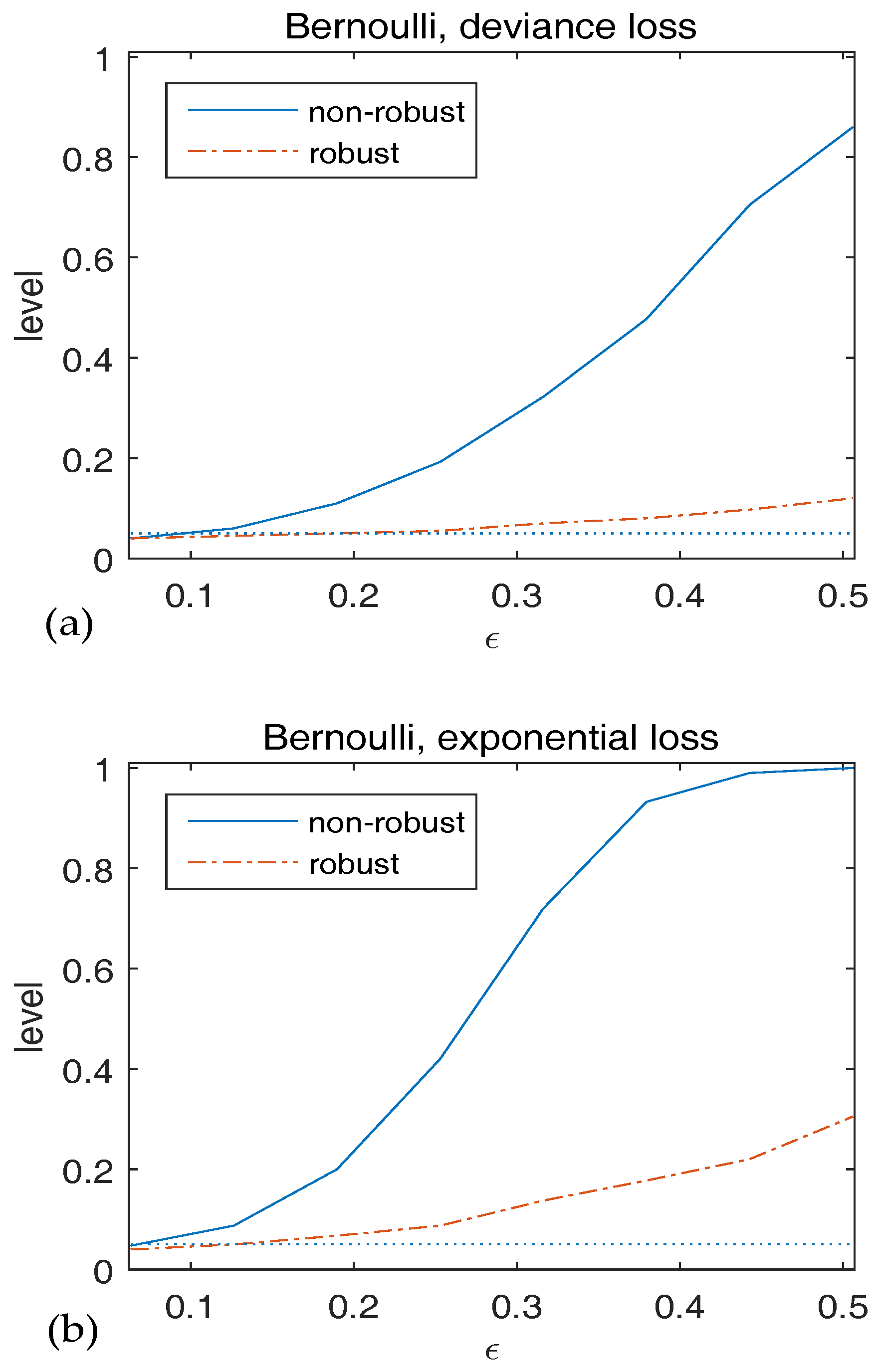
Figure 4.
Observed power of versus for Bernoulli responses. The top panels correspond to deviance loss while the bottom panels are for exponential loss. The statistics in the left panels are calculated using non-robust method and those in the right panels are from robust method. The asterisk line indicates the 5% significance level.

© 2018 by the authors. Licensee MDPI, Basel, Switzerland. This article is an open access article distributed under the terms and conditions of the Creative Commons Attribution (CC BY) license (http://creativecommons.org/licenses/by/4.0/).
Share and Cite
MDPI and ACS Style
Guo, X.; Zhang, C. Robustness Property of Robust-BD Wald-Type Test for Varying-Dimensional General Linear Models. Entropy 2018, 20, 168. https://doi.org/10.3390/e20030168
AMA Style
Guo X, Zhang C. Robustness Property of Robust-BD Wald-Type Test for Varying-Dimensional General Linear Models. Entropy. 2018; 20(3):168. https://doi.org/10.3390/e20030168
Chicago/Turabian StyleGuo, Xiao, and Chunming Zhang. 2018. "Robustness Property of Robust-BD Wald-Type Test for Varying-Dimensional General Linear Models" Entropy 20, no. 3: 168. https://doi.org/10.3390/e20030168
Note that from the first issue of 2016, this journal uses article numbers instead of page numbers. See further details here.