Optimum Criteria on the Performance of an Irreversible Braysson Heat Engine Based on the new Thermoeconomic Approach

1
Department of Physics, Xiamen University, Xiamen 361005, People's Republic of China
2
Centre for Energy Studies, Indian Institute of Technology, Delhi New Delhi 110016, India
*
Author to whom correspondence should be addressed.
Entropy 2004, 6(2), 244-256; https://doi.org/10.3390/e6020244
Submission received: 28 January 2004
/
Accepted: 8 March 2004
/
Published: 17 March 2004
Abstract
:An irreversible cycle model of a Braysson heat engine operating between two heat reservoirs is used to investigate the thermoeconomic performance of the cycle affected by the finite-rate heat transfer between the working fluid and the heat reservoirs, heat leak loss from the heat source to the ambient and the irreversibility within the cycle. The thermoeconomic objective function, defined as the total cost per unit power output, is minimized with respect to the cycle temperatures along with t he isobaric temperature ratio for a given set of operating parameters. The objective function is found to be an increasing function of the internal irreversibility parameter, economic parameters and the isobaric temperature ratio. On the other hand, there exist the optimal values of the state point temperatures, power output and thermal efficiency at which the objective function attains its minimum for a typical set of operating parameters. Moreover, the objective function and the corresponding power output are also plotted against the state point temperature and thermal efficiency for a different set of operating parameters. The optimally operating regions of these important parameters in the cycle are also determined. The results obtained here may provide some useful criteria for the optimal design and performance improvements, from the point of view of economics as well as from the point of view of thermodynamics of an irreversible Braysson heat engine cycle and other similar cycles as well.
Introduction
The Braysson cycle is a hybrid power cycle based on a conventional Brayton cycle for the high tempe rature heat addition while adopting the Ericsson cycle for the low temperature heat rejection as proposed and investigated by Frost et al. [1] using the first law of thermodynamics. Very recently, some workers [2,3] have investigated the performance of an endoreversible Braysson cycle based on the analysis of the Brayton [4,5,6,7,8,9,10,11,12,13,14,15,16,17,18,19,20,21,22,23] and Ericsson [24,25,26,27,28] cycles using the concept of finite time thermodynamics [29,30,31,32,33] for a typical set of operating conditions and obtained some significant results.
In real thermodynamic cycles, there often exist other irreversibilities besides finite-rate heat transfer between the working fluid and the heat reservoirs. For example, the heat leak loss from the heat source to the ambient and the internal dissipation of the working fluid are also another main source of irreversibility. In the present paper, we will study the influence of multi-irreversibilities on the thermoeconomic performance of a Braysson heat engine cycle.
An Irreversible Braysson Cycle
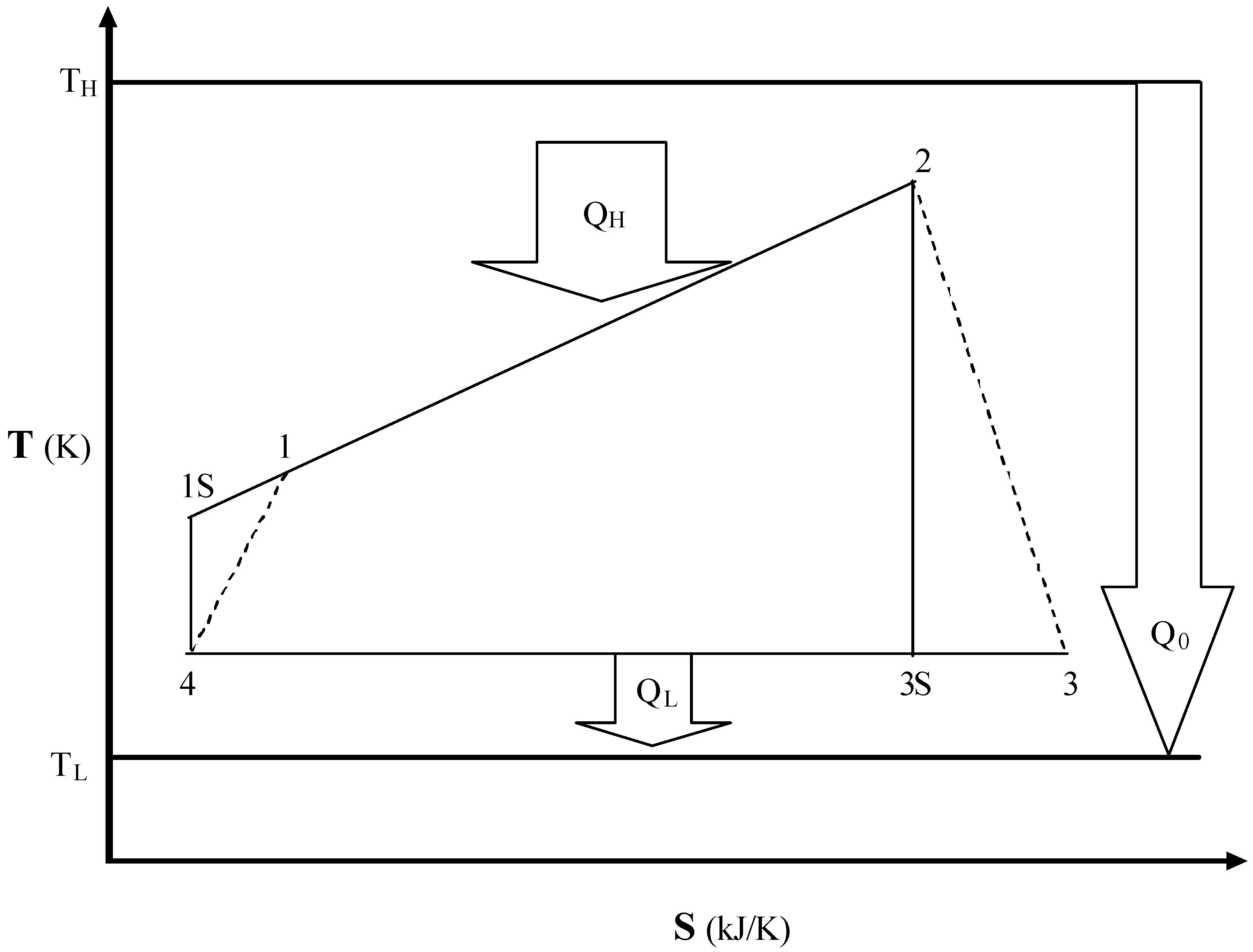
An irreversible Braysson cycle working between a source and a sink of infinite heat capacities is shown on the T-S diagram of Fig.1. The external irreversibilities are due to the finite temperature difference between the heat engine and the external reservoirs and the direct heat le ak loss from the source to the ambient while the internal irreversibilities are due to the nonisentropic processes in the expander and compressor devices as well as due to other entropy generations within the cycle. The working fluid enters the compressor at state point 4 and is compressed up to state point 1S/1 in an ideal/real compressor, and then it comes into contact with the heat source and is heated up to state point 2 at constant pressure. After that the working fluid enters the turbine at state point 2 and expands up to state point 3S/3 in an ideal/real expander/turbine, it rejects the heat to the heat sink at constant temperature and enters the compressor at state point 4, thereby, completing the cycle. Thus, we will study the 4-1-2-3-4 closed cycle of an irreversible Braysson heat engine coupled with the heat reservoirs of infinite heat capacities at temperature TH and TL respectively.
Assuming the working fluid as an ideal/prefect gas, the heat transfer rates to and from the heat engine following Newton’s Law of heat transfer [1,2,3,30,31,32,33,34,35,36] will be:
![Entropy 06 00244 i001]() where (UA)J (J = H, L) are the overall heat transfer coefficient-area products on their respective side heat exchanger, Ti (i = 1, 2,3) are the temperatures of the working fluid at state points 1, 2 and 3, and and CP are, respectively, the mass flow rate and specific heat of the working fluid.
where (UA)J (J = H, L) are the overall heat transfer coefficient-area products on their respective side heat exchanger, Ti (i = 1, 2,3) are the temperatures of the working fluid at state points 1, 2 and 3, and and CP are, respectively, the mass flow rate and specific heat of the working fluid.

According to Fig.1, It is reasonable to consider some heat leak loss directly from the source to the ambient, which may be expressed as [27]:
where k0 is the heat leak coefficient and Ta is the ambient temperature and is usually the same as the sink temperature (TL). In addition, it is also very important to further consider the influence of irreversible adiabatic processes and other entropy generations within the cycle. Assuming the working fluid as an ideal gas, the entropy production for the process 1-2 at constant pressure is:
where x = T2/T1 is the isobaric temperature ratio. Using the second law of thermodynamics for this cycle model, we have:
![Entropy 06 00244 i002]() where R is the internal irreversibility parameter which is greater than unity for a real cycle and defined as:
where R is the internal irreversibility parameter which is greater than unity for a real cycle and defined as:
![Entropy 06 00244 i003]()

When the adiabatic processes are reversible and other entropy generations within the cycle are negligible, R = 1 and the cycle becomes an endoreversible cycle, in which the irreversibility is only due to finite temperature differences between the heat engine and the external reservoirs and the heat leak loss directly from the heat source to the ambient.
The Expressions of Several Parameters
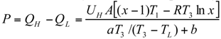
Using Eqs.(1) -(3) and (5), we can derive the expressions of the power output and thermal efficiency, which are, respectively, given by:
![Entropy 06 00244 i004]()
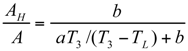
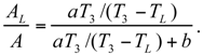
![Entropy 06 00244 i005]() where a = (UH/UL)Rln x, b = ln[(TH − T1)/(TH − T1x)] and A = AH + AL is the total heat transfer area of the cycle. Using Eqs.(1-2) and (5), we can also derive the expressions of the ratios of the hot- and cold-side heat exchanger areas to the total heat exchanger area as:
where a = (UH/UL)Rln x, b = ln[(TH − T1)/(TH − T1x)] and A = AH + AL is the total heat transfer area of the cycle. Using Eqs.(1-2) and (5), we can also derive the expressions of the ratios of the hot- and cold-side heat exchanger areas to the total heat exchanger area as:
![Entropy 06 00244 i006]()
![Entropy 06 00244 i007]()

The Thermoeconomic Objective Function
Let Cr be the total cost of the heat engine system per unit time, which includes the costs of the hot- and cold-side heat exchangers (C1), the costs of the compression/expansion device (C2), the input energy cost (C3) and the maintenance cost (C4) of the system in such a way that these costs are proportional to the total conductance, the compression/expansion capacity, the amount of heat supplied by the heat source per cycle and the power output of the cycle respectively, viz. C1 ∝ UA, C2 ∝ P, C3 ∝ (QH + Q0) and C4 ∝ P. Thus, the total cost of the system can be expressed as:
![Entropy 06 00244 i008]() where aH and aL are the proportional coefficients of the cost of the hot- and cold-side heat exchangers respectively, their units are NCU/(s-kW/K), ap, aq and am is the proportional coefficients of the costs of the compression/expansion device, input energy and maintenance, and their dimensions are NCU/(s-kW), here NCU is the National Currency Unit. Using Eqs.(1-2 and 5) and substituting k1 = aL / aH, k2 = (aP + am)/aH and k3 = aq / aH into Eq.10(a), we have:
where aH and aL are the proportional coefficients of the cost of the hot- and cold-side heat exchangers respectively, their units are NCU/(s-kW/K), ap, aq and am is the proportional coefficients of the costs of the compression/expansion device, input energy and maintenance, and their dimensions are NCU/(s-kW), here NCU is the National Currency Unit. Using Eqs.(1-2 and 5) and substituting k1 = aL / aH, k2 = (aP + am)/aH and k3 = aq / aH into Eq.10(a), we have:
![Entropy 06 00244 i009]() where k4 = k2 + k3, k5 = k3u(TH − TL) and u = k0/(THA). Again using Eqs.(1-2 and 5) and the first law of thermodynamics, yields:
where k4 = k2 + k3, k5 = k3u(TH − TL) and u = k0/(THA). Again using Eqs.(1-2 and 5) and the first law of thermodynamics, yields:
![Entropy 06 00244 i010]()


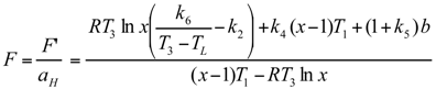
Using Eqs.10(b) and (11), the total cost of the system per unit work output may be expressed as F′ = CT / P. For the sake of simplification, the objective function F′ can be changed as: changed as:
![Entropy 06 00244 i011]() where k6 = k1 + k5UH / UL while F is referred to as the thermoeconomic objective function of an irreversible Braysson heat engine. The objective function defined in Eq.(12) is more general than those used by the earlier workers [35, 36]. For example, if R = x = 1 and aP = aq = am = Q0 = 0 are chosen, then 1/F becomes the objective function used in Ref.[35]. When R = x = 1 , aH = aL and aP = am = Q0 = 0 are chosen, F becomes the objective function used in Ref. [36]. Again, if x = 1 and other parameters are same, this cycle model will reduce to an irreversible Carnot cycle.
where k6 = k1 + k5UH / UL while F is referred to as the thermoeconomic objective function of an irreversible Braysson heat engine. The objective function defined in Eq.(12) is more general than those used by the earlier workers [35, 36]. For example, if R = x = 1 and aP = aq = am = Q0 = 0 are chosen, then 1/F becomes the objective function used in Ref.[35]. When R = x = 1 , aH = aL and aP = am = Q0 = 0 are chosen, F becomes the objective function used in Ref. [36]. Again, if x = 1 and other parameters are same, this cycle model will reduce to an irreversible Carnot cycle.
Using the above equations, one can analyze the optimal performance of an irreversible Braysson heat engine cycle.
Optimal Performance Characteristics
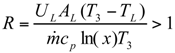
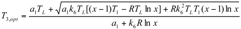
It is seen from Eq.(12) that the objective function is a function of two variables (T1, T3) for given values of the isobaric temperature ratio x and other parameters. Using Eq.(12) and its extremal condition ∂F/∂T3 = 0, it can be proven that when the objective function is in the optimal states, the temperature T3 should satisfy the following equation:
![Entropy 06 00244 i012]() where a1 = (1 + k5)b + k3(x− 1)T1. Using Eqs.(6, 12, 13), one can generate the graphs between the objective function and the state point temperature (T1), between the corresponding power output and the state point temperature (T1), between the objective function and corresponding thermal efficiency, between the objective function and corresponding power output as well as between the corresponding power output and corresponding thermal efficiency for a typical set of parameters viz. TH = 1200 K, TL = Ta = 300 K, UH / UL = 1.0, k1 = 1.1, k2 = 0.6, k3 = 0.5 and u = 0.01 , as shown in Fig.1, Fig.2, Fig.3, Fig.4 and Fig.5, where , Pm is the power output corresponding to the minimum objective function, and and are, respectively, the maximum values of the thermal efficiency and power output at the minimum objective function.
where a1 = (1 + k5)b + k3(x− 1)T1. Using Eqs.(6, 12, 13), one can generate the graphs between the objective function and the state point temperature (T1), between the corresponding power output and the state point temperature (T1), between the objective function and corresponding thermal efficiency, between the objective function and corresponding power output as well as between the corresponding power output and corresponding thermal efficiency for a typical set of parameters viz. TH = 1200 K, TL = Ta = 300 K, UH / UL = 1.0, k1 = 1.1, k2 = 0.6, k3 = 0.5 and u = 0.01 , as shown in Fig.1, Fig.2, Fig.3, Fig.4 and Fig.5, where , Pm is the power output corresponding to the minimum objective function, and and are, respectively, the maximum values of the thermal efficiency and power output at the minimum objective function.
Minimum Value of Objective Function
The variations of the objective function and the corresponding dimensionless power output against the state point temperature (T1) are shown in Fig.2 and Fig.3. It is seen from these figures that the objective function first decreases and then increases while the corresponding power output first increases and then decreases as T1 increases. It shows clearly that there are optimal values of T1 at which the objective function and the corresponding power output attain the minimum and maximum values for a given set of operating parameters, respectively. Also the optimal values of T1 are different for different parameters at different operating condition.
For example, the optimal value of T1 at the minimum objective function is greater than that of T1 at the corresponding maximum power output, i.e.
where T1,max are the maximum obtainable temperatures for a given set of operating parameters. Figure 2 and Figure 3 show that and decreases with the increase of x and increases with the increase of R. Again, it is also seen from these figures that the objective function is a monotonically increasing function of both x and R while it is reverse in the case of the corresponding power output. This point is easily expounded from the theory of thermodynamics. Because the larger the internal irreversibility parameter R and the isobaric temperature ratio x are, the larger the total irreversibility in the cycle and consequently the smaller the corresponding power output and the larger will be the cost of the system and hence, the large value of the objective function.
Effects of Economic Parameters
The variation of the objective function with respect to the state point temperature (T1) for different thermoeconomic parameters (k1, k2 and k3) are shown in Figs. 4(a-c). It is seen from these figures that the objective function first decreases and then increases as the state point temperature (T1) increases. Thus, there is an optimal value of the state point temperature (T1) at which the objective function attains its minimum for a giv en set of operating parameters and the optimum value of T1 and hence the minima of the objective function will change if any operating parameter of the cycle is changed. Again the objective function goes up as any one of the economic parameters increases but the effects of k2 and k3 are more than those of k1 on the objective function at the same set of operating condition.
Objective Function, Corresponding Power Output and Thermal Efficiency
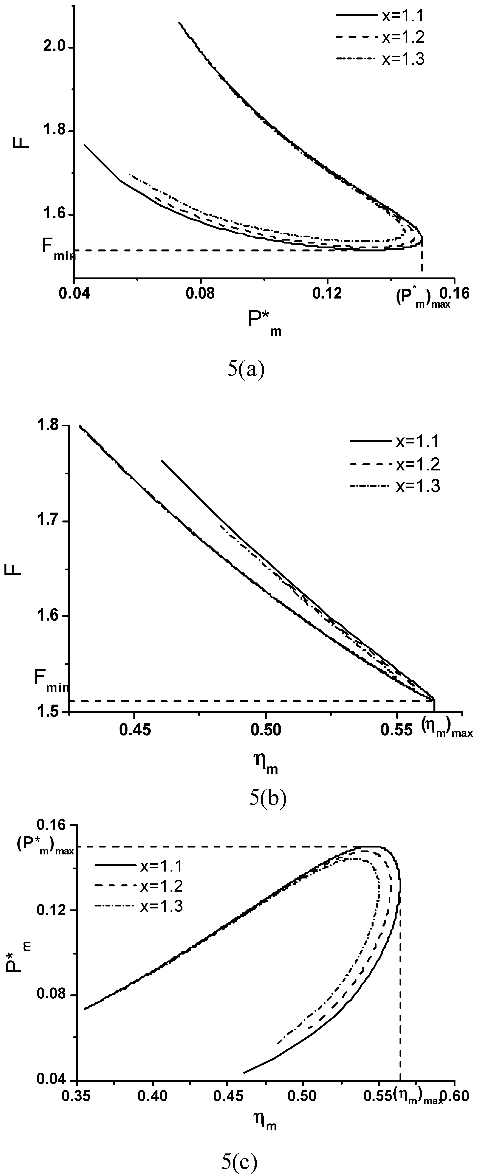
Figure 5(a-c) show the , and curves, which may be used to further reveal the performance characteristics of an irreversible Braysson cycle. It is seen from these figures that the objective function is not a monotonic function of the power output and thermal efficiency and hence, there are optimal values of the power output and thermal efficiency at which the objective function attains its minimum values. Also the optimum operating regions of the objective function are situated in the regions of the and curves with positive slopes.
Again, it is seen from Fig.5(c) that the corresponding power output is not a monotonic function of the corresponding thermal efficiency. When the power output is situated in the regions of the curves with a positive slope, it will decrease as the thermal efficiency is decreased. Obviously, these regions are not optimal. It is thus clear that the power output should be situated in the region of the curves with a negative slope. When the power output is in the region, it will increase as the thermal efficiency is decreased, and vice-versa. Thus, the optimal operating region of the objective function, power output and thermal efficiency are given by:
This shows that , , , , and are the important optimal performance parameters of the Braysson heat engine. Thus and give the upper bounds of the power output and thermal efficiency at the minimized objective function, while and determine the values of the power output and thermal efficiency at the point of Fmin.On the other hand, and give the allowable values of the lower bounds of the power output and therma l efficiency at the minimized objective function.
According to Eqs.(8-9), we can further determine the optimal regions of other performance parameters. For example, the optimal regions of the parameters AH / A and AL / A may be, respectively, determined by:
where (AH / A)F, (AL / A)F, , and , are, respectively, the values of the AH / A and AL / A at the minimum objective function and the corresponding maximum specific power output and thermal efficiency.
So far we have obtained some optimum criteria for the important performance parameters of the cycle and found that the point of the minimum objective function is just in the optimal operating region, which may provide some important theoretical guidance for the design and improvement of an irreversible Braysson cycle.
A Special Case
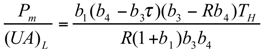
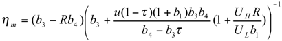
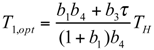
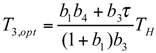
When x = 1, the present cycle model becomes a finite time Carnot cycle [29,30] with internal irreversibility [31] and consequently, the performance of the Carnot cycle can be directly obtained from the above results as follows:
![Entropy 06 00244 i013]()
![Entropy 06 00244 i014]()
![Entropy 06 00244 i015]()
![Entropy 06 00244 i016]()
![Entropy 06 00244 i017]()
![Entropy 06 00244 i018]() where
where ![Entropy 06 00244 i019]() and
and ![Entropy 06 00244 i020]()


 and
and 
It is clear that the results obtained in Refs.[35, 36] may be directly derived from the above equations.
From these results mentioned above, we can conclude that the parameters viz. the objective function as well as the corresponding power output of the Carnot cycle is, respectively, smaller and larger than those of the Braysson cycle for the same set of operating parameters. Since, the objective function defined in this paper should be as less as possible (but not zero) from the point of view of economics for a given set of operating parameters. Thus, the Carnot cycle can exhibit better performance than the Braysson cycle for the same set of operating parameters not only from the point of view of thermodynamics but also from the point of view of thermoeconomics.
Conclusions
An irreversible cycle model of a Braysson heat engine is established and used to investigate the influence of multi-irreversibilities on the thermoeconomic objective function of the heat engine. The objective function is optimized with respect to the cycle temperatures for a given set of operating parameters. The minimum objective function and the corresponding power output as well as some other important parameters are calculated for a typical set of operating conditions. The optimal regions of some important parameters such as the objective function, corresponding power output and thermal efficiency, state point temperatures of the working fluid, heat-transfer area ratios, and so on, are determined in detail. The influence of the isobaric temperature ratio (x) and internal irreversibility parameter (R) on the performance of the cycle is analyzed. The objective function is found to be an increasing function of the internal irreversibility parameter, economic parameters and the isobaric temperature ratio. On the other hand, there exist the optimal values of the state point temperatures , power output and thermal efficiency at which the objective function attains its minimum for a typical set of operating parameters. A special case of the cycle is also discussed which indicates that the optimal thermoeconomic performance of an irreversible Carnot heat engine may be directly derived from the results obtained in this paper. In other words, the analysis presented in this paper is general and will be useful to understand the relationships and difference between the Braysson cycle and other cycles and to further improve the optimal design and operation from the point of view of economics as well as from the point of view of thermodynamics of a Braysson heat engine for the different set of operating parameters and for given constraints.
Acknowledgement
One of the authors (S K Tyagi) gratefully acknowledges the financial assistance and working opportunity provided by Xiamen University, Xiamen, People’s Republic of China, during this study.
Nomenclature
| NCU = National Currency Unit | |
| A = Area (m2) | P = Power output (kW) |
| a’s = Cost parameters | P* =Dimensionless power output |
| cp = Specific heat (kJ/kg-K) | Q = Heat transfer rates (kW) |
| C’s = Cost parameters | R = Internal irreversibility parameter |
| CT = Total cost (defined in Eq.10) | S = Entropy (kJ/K) |
| F = Objective function (defined in Eq.12) | T = Temperature (K) |
| U = Overall heat transfer coefficient (kW/m2-KL) = Sink/cold -side | |
| x = Isobaric temperature ratio | m=Related to the minimum objective |
| 1, 2, 3, 4 = State points | function/maintenance |
| Greeks | max = Maximum |
| η = Efficiency | min = Minimum |
| Subscripts | opt = Optimum |
| a = Ambient | p = Related to power production cost |
| c = Compressor | q = Related to input energy rate cost |
| H = Heat source/hot -side | |
References
- Frost, T. H.; Anderson, A.; Agnew, B. A hybrid gas turbine cycle (Brayton/Ericsson): an alternative to conventional combined gas and steam turbine power plant. Proc. Inst. Mech. Eng. Part A 1997, 211, 121–131. [Google Scholar] [CrossRef]
- Zheng, T.; Chen, L.; Sun, F.; Wu, C. Power, power density and efficiency optimization of an endoreversible Brays son cycle. Exergy 2002, 2, 380–386. [Google Scholar] [CrossRef]
- Zheng, J.; Chen, L.; Sun, F.; Wu, C. Powers and efficiency performance of an endoreversible Braysson cycle. Int. J. Therm. Sci. 2002, 41, 201–205. [Google Scholar] [CrossRef]
- Wu, C.; Kiang, R. S. Work and power optimization of a finite time Brayton cycle. Int. J. Ambient Energy 1990, 11, 129–136. [Google Scholar] [CrossRef]
- Wu, C.; Kiang, R. S. Power performance of a nonisentropic Brayton cycle, J. Eng. Gas Turbines Power 1991, 113, 501–504. [Google Scholar] [CrossRef]
- Leff, H. S. Thermal efficiency at maximum power output: New results for old engines. Am. J. Phys. 1987, 55, 602–610. [Google Scholar] [CrossRef]
- Ibrahim, O. M.; Klein, S. A.; Mitchell, J. W. Optimum heat power cycles for specified boundary conditions. J. Eng. Gas Turbines Power 1991, 113, 514–521. [Google Scholar] [CrossRef]
- Wu, C. Specific power bounds of real heat engines. Energy Convers. Mgmt. 1991, 31, 249–253. [Google Scholar] [CrossRef]
- Wu, C. Power optimization of an endoreversible Brayton gas heat engine. Energy Convers. Mgmt. 1991, 31, 561–565. [Google Scholar] [CrossRef]
- Wu, C.; Chen, L.; Sun, F. Performance of a regenerative Brayton heat engine. Energy 1996, 21, 71–76. [Google Scholar] [CrossRef]
- Cheng, C.Y.; Chen, C.K. Power optimization of an endoreversible regenerative Brayton cycle. Energy 1996, 21, 241–247. [Google Scholar] [CrossRef]
- Chen, L.; Sun, F.; Wu, C.; Kiang, R. L. Theoretical analysis of the performance of a regenerative closed Brayton cycle with internal irreversibilities. Energy Convers. Mgmt. 1997, 38, 871–877. [Google Scholar] [CrossRef]
- Radcenco, V.; Vargas, J. V. C.; Bejan, A. Thermodynamic optimization of a gas turbine power plant with pressure drop irreversibilities. J. Energy Res. Tech. 1998, 129, 233–240. [Google Scholar] [CrossRef]
- Blank, D. A. Analysis of a combined law power optimized open Joule -Brayton heat engine cycle with a finite interactive heat source. J. Phys. D: Appl. Phys. 1999, 32, 769–776. [Google Scholar] [CrossRef]
- Sahin, B.; Kodal, A.; Kaya, S. S. A comparative performance analysis of irreversible regenerative reheating Joule-Brayton heat engine under maximum power density and maximum power conditions. J. Phys D: Appl. Phys. 1998, 31, 2125–2131. [Google Scholar] [CrossRef]
- Roco, J. M. M.; Velasco, S.; Medina, A.; Hernandez, A. C. Optimum performance of a regenerative Brayton thermal cycle. J. Appl. Phys. 1997, 82, 2735–2741. [Google Scholar] [CrossRef]
- Feidt, M. Optimization of Brayton cycle engine in contract with fluid thermal capacities. Rev. Gen. Them. 1996, 35, 662–666. [Google Scholar] [CrossRef]
- Chen, L.; Ni, N.; Cheng, G.; Sun, F.; Wu, C. Performance of a real closed regenerated Brayton cycle via method of finite time thermodynamics. Int. J. Ambient Energy 1999, 20, 95–104. [Google Scholar] [CrossRef]
- Cheng, C. Y.; Chen, C. K. Power optimization of an irreversible Brayton heat engine. Energy Sources 1997, 19, 461–474. [Google Scholar] [CrossRef]
- Blank, D. A.; Wu, C. A combined power optimized Joule -Brayton heat engine cycle with fixed thermal reservoir. Int. J. Power and Energy 2000, 20, 1–6. [Google Scholar]
- Frost, T. H.; Agnew, B.; Anderson, A. Optimizations for Brayton-Joule gas turbine cycles. Proc. Inst. Mech. Eng. Part A: J. Power and Energy 1992, 206, 283–288. [Google Scholar] [CrossRef]
- Horlock, J. H.; Woods, W. A. Determination of the optimum performance of gas turbine. Proc. Inst. Mech. Eng. Part C: J. Mech. Sci. 2000, 214, 243–255. [Google Scholar] [CrossRef]
- Kaushik, S. C.; Tyagi, S. K. Finite time thermodynamic analysis of an irreversible regenerative closed Brayton cycle heat engine. Int. J. Solar Energy 2002, 22, 141–151. [Google Scholar] [CrossRef]
- Blank, D. A.; Wu, C. Power limit of an endoreversible Ericsson cycle with regeneration. Energy Convers. Mgmt. 1996, 37, 59–66. [Google Scholar] [CrossRef]
- Blank, D. A.; Wu, C. Finite time power limit for solar-radiant Ericsson engines in space applications. Appl. Therm. Eng. 1998, 18, 1347–1357. [Google Scholar] [CrossRef]
- Chen, J.; Schouten, J. A. The comprehensive influence of several major irreversibilities on the performance of an Ericsson heat engine. Appl. Therm. Eng. 1999, 19, 555–564. [Google Scholar] [CrossRef]
- Tyagi, S. K. Application of finite time thermodynamics and second law evaluation of thermal energy conversion systems. Ph. D. Thesis, CCS. University, Meerut, India, 2000. [Google Scholar]
- Kaushik, S. C.; Kumar, S. Finite time thermodynamic evaluation of irreversible Ericsson and Stirling heat engines. Energy Convers. Mgmt. 2001, 42, 295–312. [Google Scholar] [CrossRef]
- Curzon, F. L.; Ahlborn, B. Efficiency of Carnot engine at maximum power output. Am. J. Phys. 1975, 19, 22–24. [Google Scholar] [CrossRef]
- Bejan, A. Theory of heat transfer irreversible power plants. Int. J. Heat Mass Transfer 1988, 31, 1211–1219. [Google Scholar] [CrossRef]
- Wu, C.; Kiang, R. L. Finite time thermodynamic analysis of a finite time Carnot heat engine with internal irreversibility. Energy 1992, 17, 1173–1178. [Google Scholar] [CrossRef]
- Chen, J. The maximum power output and maximum efficiency of an irreversible Carnot heat engine. J. Phys. D: Appl. Phys. 1994, 27, 1144–1149. [Google Scholar] [CrossRef]
- Chen, J. Thermodynamic and thermoeconomic analyses of an irreversible combined Carnot heat engine system. Int. J. Energy Res. 2001, 25, 413–426. [Google Scholar] [CrossRef]
- Kodal, A.; Sahin, B.; Yilmaz, T. Effects of internal irreversibility and heat leakage on the finite time thermoeconomic performance of refrigerators and heat pumps. Energy Convers. Mgmt. 2000, 41, 607–619. [Google Scholar] [CrossRef]
- Sahin, B.; Kodal, A. Performance analysis of an endoreversible heat engine based on a new thermoeconomic optimization criterion. Energy Convers. Mgmt. 2001, 42, 1085–1093. [Google Scholar] [CrossRef]
- Antar, M. A.; Zubair, S. M. Thermoeconomic considerations in the optimum allocation of heat exchanger inventory for a power plant. Energy Convers. Mgmt. 2001, 42, 1169–1179. [Google Scholar] [CrossRef]
Fig.1.
The T-S diagram of an irreversible Braysson heat engine cycle.

Fig.2.
The variation of (a) the objective function and (b) the corresponding power output with respect to temperature T1 for different values of the isobaric temperature ratio (x), where the parameters TH = 1200 K, TL = 300 K, R = 1.1, UH / UL = 1.0, k1 = 1.1, k2 = 0.6, k3 = 0.5 and u = 0.01 are chosen.
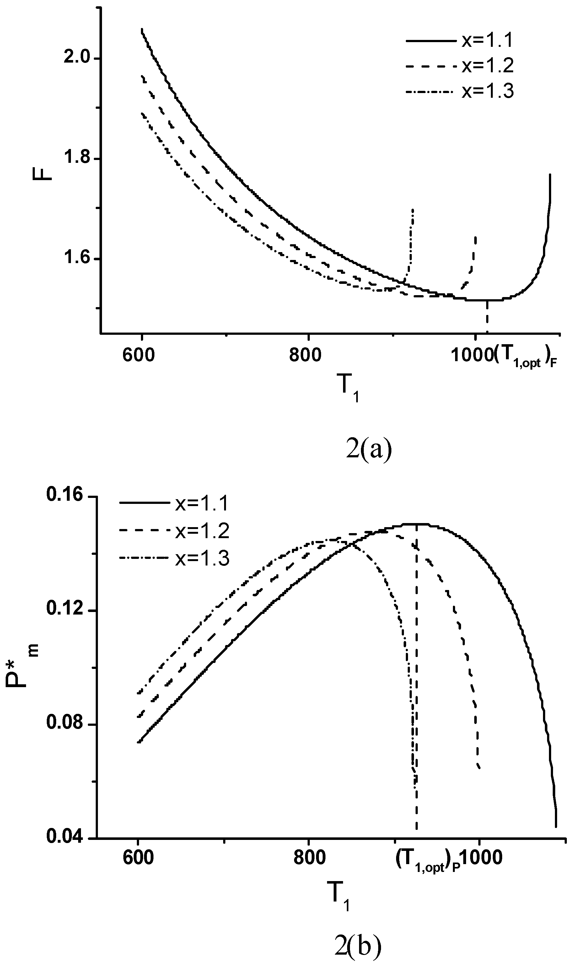
Fig.3.
The variation of (a) the objective function and (b) the corresponding power output with respect to temperature T1 for different values of R, where x = 1.1 and the values of the parameters are the same as those used in Fig. 2.
Fig.3.
The variation of (a) the objective function and (b) the corresponding power output with respect to temperature T1 for different values of R, where x = 1.1 and the values of the parameters are the same as those used in Fig. 2.
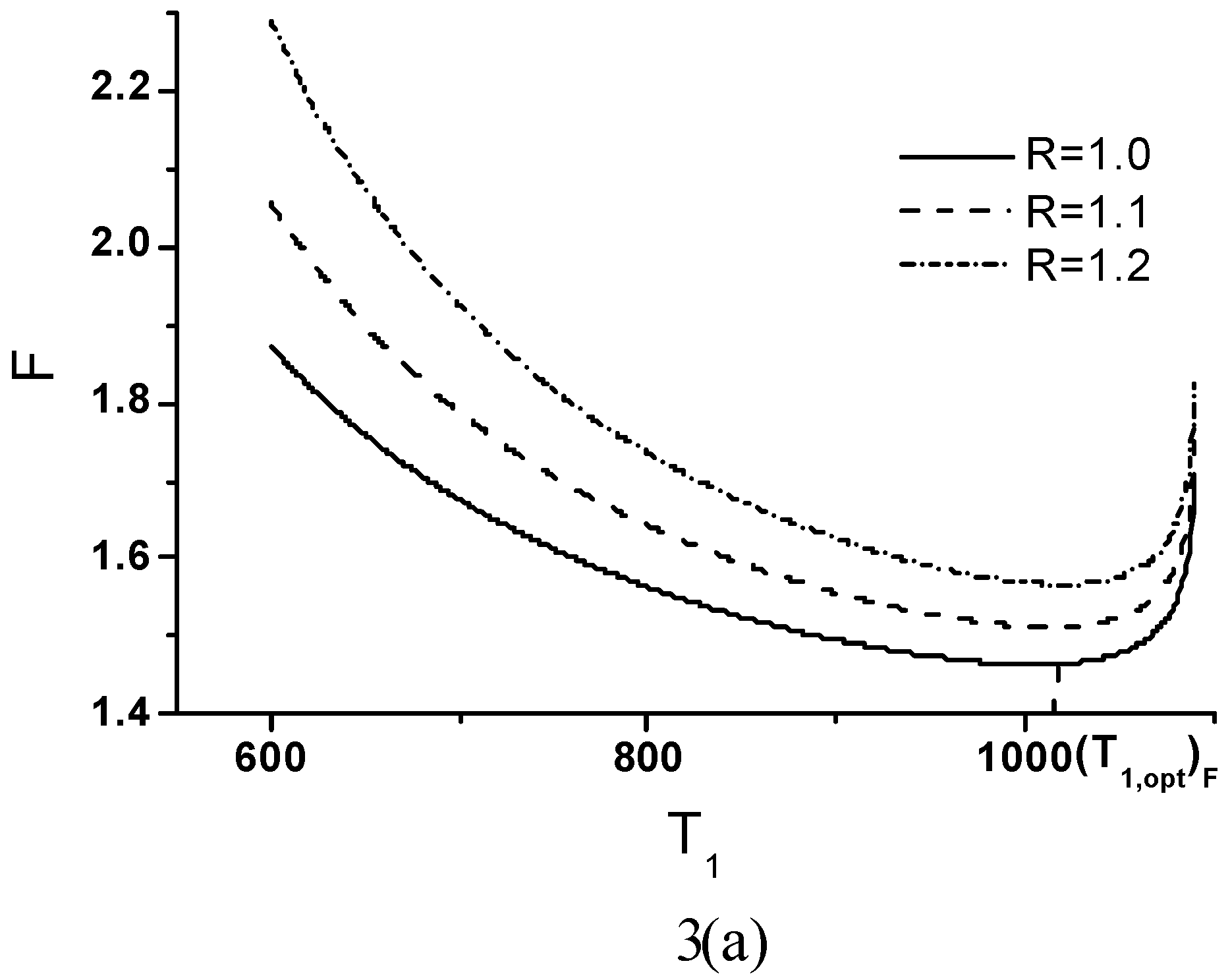
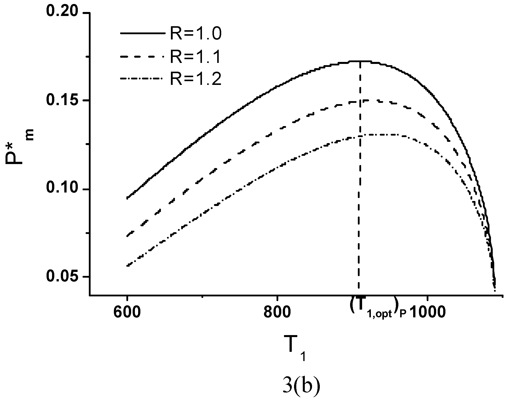
Fig.4.
The variation of the objective function with res pect to temperature T1 for different parameters (a) k1, (b) k2 and (c) k3, where x = R = 1.1 and the values of the parameters are the same as those used in Fig. 2.
Fig.4.
The variation of the objective function with res pect to temperature T1 for different parameters (a) k1, (b) k2 and (c) k3, where x = R = 1.1 and the values of the parameters are the same as those used in Fig. 2.
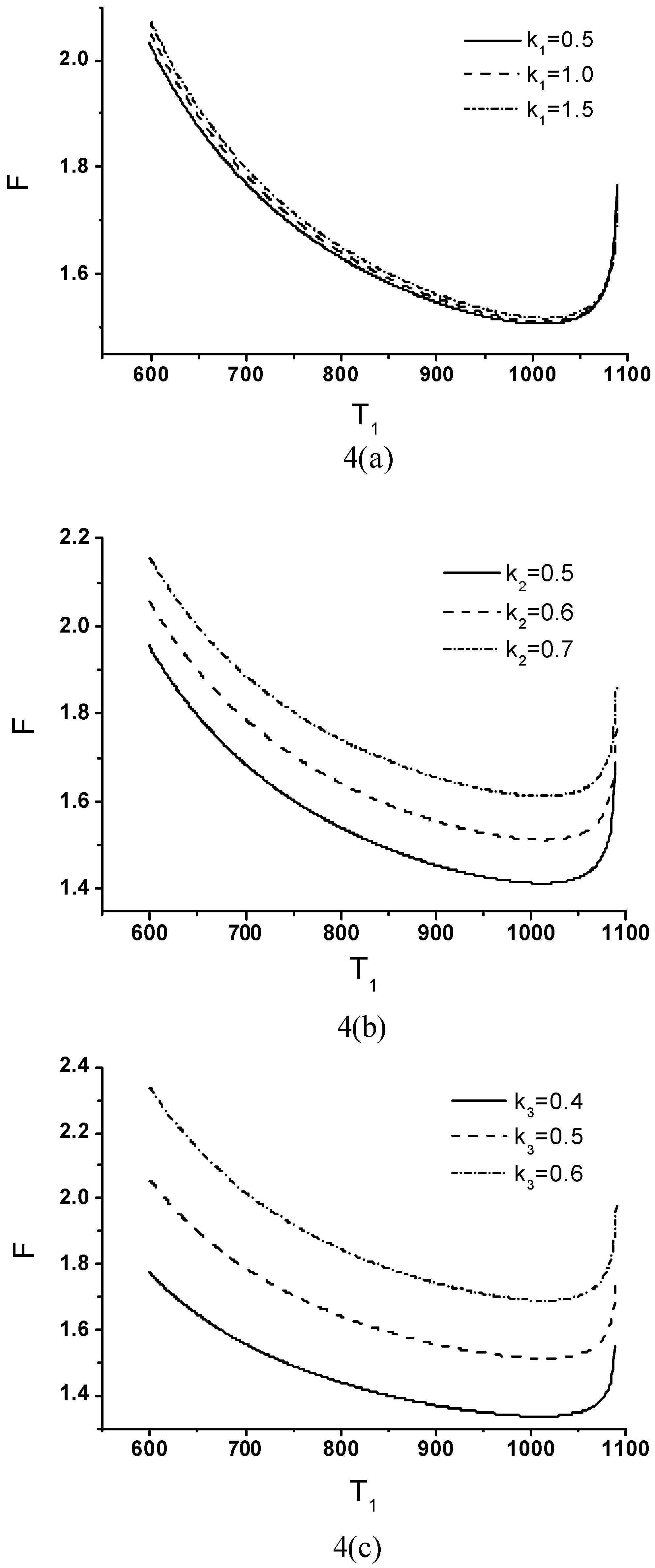
Fig.5.
The (a) , (b) and curves of a Braysson heat engine, where the values of the parameters are the same as those used in Fig. 2.
Fig.5.
The (a) , (b) and curves of a Braysson heat engine, where the values of the parameters are the same as those used in Fig. 2.

© 2004 by MDPI (http://www.mdpi.org). Reproduction for noncommercial purposes permitted.
Share and Cite
MDPI and ACS Style
Tyagi, S.K.; Zhou, Y.; Chen, J. Optimum Criteria on the Performance of an Irreversible Braysson Heat Engine Based on the new Thermoeconomic Approach. Entropy 2004, 6, 244-256. https://doi.org/10.3390/e6020244
AMA Style
Tyagi SK, Zhou Y, Chen J. Optimum Criteria on the Performance of an Irreversible Braysson Heat Engine Based on the new Thermoeconomic Approach. Entropy. 2004; 6(2):244-256. https://doi.org/10.3390/e6020244
Chicago/Turabian StyleTyagi, Sudhir Kumar, Yinghui Zhou, and Jincan Chen. 2004. "Optimum Criteria on the Performance of an Irreversible Braysson Heat Engine Based on the new Thermoeconomic Approach" Entropy 6, no. 2: 244-256. https://doi.org/10.3390/e6020244