Remarks on the Compatibility of Opposite Arrows of Time

Abstract

I argue that opposite arrows of time, while being logically possible, cannot realistically be assumed to exist during one and the same epoch of our universe.

1 Introduction

If, according to the assumptions of statistical physics, the second law is regarded as a “fact” rather than a dynamical law, it could conceivably not hold at all, hold only occasionally, or even apply in varying directions of time. Larry Schulman has demonstrated very nicely and convincingly in several publications [1, 2, 3] how the latter possibility may occur in principle. The major remaining question then is whether his examples can be regarded as realistic in our universe. This comment was written in response to a review presented by Schulman during a conference on the “Direction of Time”, Bielefeld (2002), and posted as http://arXiv.org/physics/0306083.

In particular, we may understand from Schulman’s examples how a certain time arrow depends on “improbable” (low entropy) initial or final conditions – regardless of the direction in which we perform our calculation. The latter (apparently trivial) remark may be in place, since many derivations of the second law tacitly assume in a crucial way that the calculation is used to predict. That is, it is assumed to follow a “physical” direction of time (from an initially given present towards an unknown future). However, precisely this physical arrow, or the fact that only the past can be remembered and appears “fixed”, is a major explanandum.

While, for a given dynamical theory, we know in general precisely what freedom of choice remains for initial or final conditions, mixed ones (such as two-time boundary conditions) are subject to dynamical consistency requirements – similar to an eigenvalue problem with given eigenvalue. This problem remains relevant even for incomplete (for example, macroscopic) initial and final conditions. It is usually difficult to construct an individual solution that is in accord with both of them. In Schulman’s examples, individual solutions were mostly found by “trial and error”, that is, by exploiting a sufficient number of solutions with given initial conditions and selecting those which happen to fulfill the final ones (or vice versa). However, in a realistic situation it would be absolutely hopeless in practice ever to end up with the required low entropy because of the exponential growth of probability with entropy. Only an exponentially small fraction of all solutions satisfies one or the other low entropy boundary conditions. In the case of complete mixing, it is the square of this very small number that measures the fraction of solutions with two-time boundary conditions.

Being able to find solutions by trial and error thus demonstrates already the unrealistic case. This difficulty in finding solutions does not present any problem for their existence on a classical continuum of states if mixing is sufficiently complete: any set of solutions with finite measure can be further partitioned at will, since entropy has no lower bound in this classical situation. This conclusion is changed in quantum theory, which would in a classical picture require the existence of elementary phase space cells of Planck size h^3N. The product of initial and final probabilities characterizing the required low-entropy may then represent a phase space volume smaller than a Planck cell – thus indicating the absence of any solution.

2 Retarded and Advanced Fields

The consistency problem in a classical setting (though without mixing) is discussed in Schulman’s “wet carpet” example, intended to prove the compatibility of two interacting systems with differ-ent, retarded or advanced, electrodynamics [2]. It is similar to an example studied by Wheeler and Feynman [4], where a charged particle, bound to pass an open trap door, is assumed to shut it before passing the door by means of advanced fields which it can create only after having passed the door. In both examples, there is but a very narrow band of consistent solutions, in Schulman’s example represented by a partly opened window. These narrow bands were found for systems which are far from thermodynamical mixing (cf.the following sections), and they may be consistent only if the model is considered in isolation. In reality, macroscopic objects always interact with their surroundings. In a causal world, this would produce “consistent documents” (not only usable ones) in the thermodynamical future. In this way, information may classically spread without limit, thus leading to inconsistencies with an opposite arrow of other systems. In quantum description, classical concepts even require the presence of irreversible decoherence, while microscopic systems would remain in quantum superpositions of all conceivable paths (see Sect.6).

Philosophers are using the term “overdetermination of the past” to characterize this aspect of causality [5, 6]. (Note that the conventional additive physical entropy neglects such nonlocal correlations, which would describe the consistency of documents, for being dynamically irrelevant in the future [7].) In a deterministic world, one would thus have to change all future effects in a consistent way in order to change the past. For example, classical light would even preserve its usable information content forever in a transparent universe. In classical electrodynamics, there is but one real Maxwell field, while the retarded and advanced fields of certain sources are merely auxiliary theoretical concepts. The same real field can be viewed as a sum of incoming and retarded, or of outgoing and advanced fields, for example (see Chap. 2 of [7]). Retarded and advanced fields (of different sources) thus do not add. Observing retarded fields (as our sensorium and other registration devices evidently do) means that incoming fields related to unspecified past sources (“noise”) are negligible – incompatible with the presence of distinctive advanced radiation. Problems similar to those with opposite arrows occur with closed time-like curves (CTCs), which are known to exist mathematically in certain solutions of Einstein’s field equations of general rel-ativity. This existence means that local initial and final conditions for the geometry, defined with respect to these closed time-like curves, are identical and thus dynamically consistent. However, CTCs are incompatible with an arrow of time for matter, such as an electrodynamic or ther-modynamic one. Those clever science fiction stories about time travel, which are constructed to circumvent paradoxes, and thus seem to allow CTCs for human adventurers, simply neglect all irreversible effects which must arise and would destroy dynamical consistency. Since geometry and matter are dynamically coupled, boundary conditions which lead to an arrow of time must also protect chronology (whatever the precise dynamical model). Wet carpet stories belong to the same category as science fiction stories: they do not resolve the unmentioned paradoxes that would necessarily arise from opposite arrows.

3 Cat Maps

Borel demonstrated long ago [8] that microscopic states of classically described gases are dynami-cally strongly coupled even over astronomical distances. This is a time-symmetric consequence of their extremely efficient chaotic behavior, caused by deterministic molecular collisions. Of course, this does not mean that macroscopic properties are similarly sensitive to small perturbations, although fluctuations (such as Brownian motion) and their concequences must be affected.

Macroscopic properties characterize the microscopic state of a physical system incompletely, for example by representing a coarse graining in phase space (or, more generally, a Zwanzig projection – Chap. 3 of [7]). The deterministic dynamics of initially given coarse grains is often described by measure-preserving dynamical maps. In contrast to deformations of extended individual objects in space (such as Gibbs’ ink drop), and even in contrast to the N discrete points in single-particle phase space which represent a molecular gas, Kac’s symbolic “cats” (areas in phase space) [11] represent ensembles, or sets, of possible physical states of a given system. Therefore, Schulman’s entropy [2] as a function of deformed cats (“cat maps”) is an ensemble (or average) entropy – not the entropy of an individual physical state. The entropy of this ensemble is defined to depend on its distribution in phase space, obtained after coarse graining with respect to given and fixed grains as a macroscopic reference system, while the entropy of an individual state (point in phase space) would be given solely by the size of the specific grain that happens to contain it at a certain time.

This is essential (and sufficient) for Schulman’s argument that the intersection of two sets rep-resenting specific initial or final conditions is not empty if mixing is complete. In our universe, however, some variables participate in very strong mixing, while others (“robust” ones, such as electromagnetic waves or atomic nuclei) may remain stable for very long times. They are the ones that may store usable information.

Since cat maps describe sets of states for rather simple dynamical systems, their dynamics is far less sensitive to weak interactions than that of individual Borel type systems. For this reason, two systems described by cat maps with opposite arrows of time may even be consistent for mild interactions [2]. However, these cat maps do not form a realistic model appropriate to discuss thermodynamical arrows in our universe.

4 (Anti-)Causality

In order to define causality without presuming a direction of time, one has to refer to the inter-nal structure of the evolving dynamical states. The above-mentioned over-determination of the past (in other words, the existence and consistency of multiple documents) is a typical example. Another one is given by the concentric waves emitted from a local source. In our world, both are empirically (not logically) related to a time direction.

While one may expect that all such internal structures can be shown to evolve in time from appropriate initial conditions, they are too complex to be investigated in terms of Schulman’s simple models. For example, retarded (concentrically outgoing) waves exist in the presence of sources precisely when incoming fields are negligible. This can be the case “because” of an initial condition for the fields, or because of the presence of thermodynamic absorbers [7].

Instead of these specific structures of physical states, Schulman studied the “effect” (in both directions of time) of “perturbations” defined by small instantaneous changes of the Hamiltonian [3]. This “effect” is not easily defined in a time-symmetric way, since an “unperturbed solution” defined on one temporal side of the perturbation would be exclusively changed on the other one (no matter which is the future or past). If the unperturbed solution obeyed a two-time boundary condition, the perturbed one would in general violate it on this “other” temporal side. In contrast to the above mentioned internal structures, our conventional concept of perturbations is based on the time direction used in the definition of external operations.

Therefore, in a first step, Schulman considered sets of solutions again. The set of all solutions obeying the “left” boundary condition (in time) remains unchanged on the left of the perturbation, while the opposite statement is true on the right. However, individual solutions found in the intersection of these two sets (consisting of those ones which fulfill both boundary conditions) in the case of a perturbation are generically different from the unperturbed ones on both sides of the perturbation. Now, if mixing is essentially complete on the right of the perturbation (that is, for a sufficiently distant right boundary), the right boundary condition does not affect the solutions which form the intersection (considered as a set) on the left. This means that mean values of macroscopic variables in the set of all solutions that are compatible with both boundary conditions may only differ on the right (a consequence regarded as causality by Schulman) [3]. This is true, in particular, for the mean entropy (if the latter is defined as a function of macroscopic, that is coarse-grained, variables). Individual solutions can not be compared in this way, since there is no individual relation between them. In the case of complete mixing on the right, there is even a small but non-empty subset of solutions of the original two-time boundary value problem which keep obeying the right boundary condition without being changed on the left. However, using them for the argument would mean that only very specific solutions can be perturbed in this specific sense.

In a second approach, Schulman studies the “effect” of macroscopic perturbations on individual solutions of an integrable system. This system is defined as consisting of a finite number of in-dependent oscillators with different frequencies. Although solutions which fulfill both boundary conditions can be found with and without an appropriate perturbation, they are again not indi-vidually related. Therefore, the causal interpretation of the perturbation remains obscure. (For closed deterministic systems, any perturbation would itself have to be determined from micro-scopic boundary conditions, and the consistency problem becomes even more restrictive than for just two boundary conditions.)

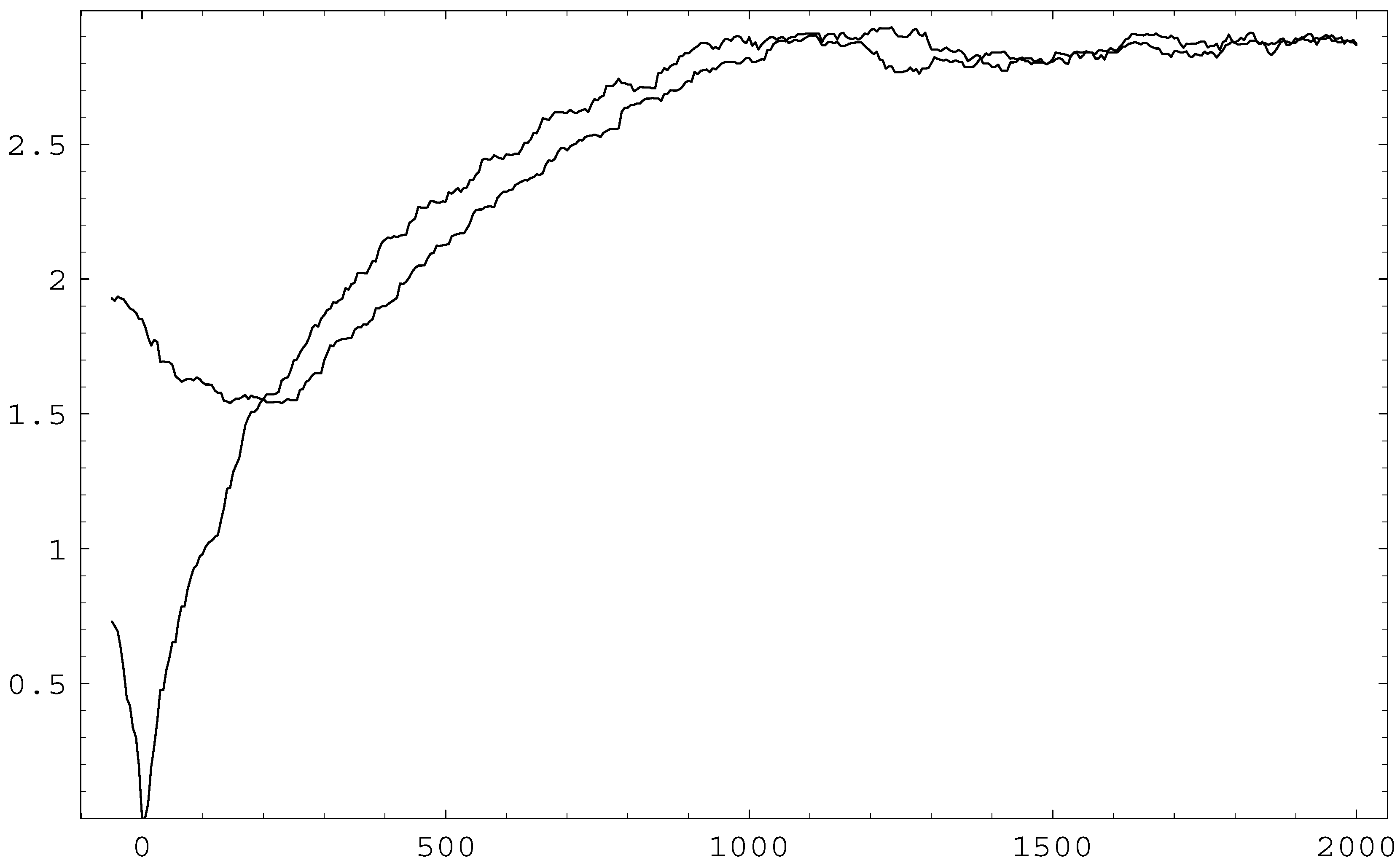
Nonetheless, I was pleased to discover that Schulman’s model is formally identical with a model of particles freely moving on a periodic interval (a “ring”) that I had used in an appendix of [7] for much larger numbers of constituents than used by him (such that finding two-time boundary solutions by trial and error would be hopeless). Particle positions on the ring have merely to be re-interpreted as oscillator amplitudes in order to arrive at Schulman’s picture. I used this opportunity to search by trial and error among analytically constructed two-time boundary solu-tions for those ones which happen to possess slightly lower entropy than the mean at some given “perturbation time” t₀ (see Fig. 1). (Finding much lower entropy values numerically would be too time-consuming for this large number of particles.) Unfortunately, the results do not confirm Schulman’s claim that these solutions are “affected” by the perturbation only in the direction away from the relevant low entropy boundary (that is, towards the “physical future”) [3]. Evidently, this concept of causality, defined by means of perturbations, is insufficient. The very concept of a “perturbation” seems to be ill-defined for two-time boundary conditions.

Figure 1. Four random two-time boundary solutions (forming a narrow bundle in the diagram) are compared with two other ones, selected by trial and error for their slightly lower entropy values at t₀ = 200 or t₀ = −200. Values for t < 0 are identical with those at t_f − t = 200.000 − t, although the final condition is actually irrelevant in the range shown. Entropy scattering around t = 1300 is accidental. (See Appendix of [7] for details of the model and an elementary Mathematica program for your convenience.)

Figure 1. Four random two-time boundary solutions (forming a narrow bundle in the diagram) are compared with two other ones, selected by trial and error for their slightly lower entropy values at t₀ = 200 or t₀ = −200. Values for t < 0 are identical with those at t_f − t = 200.000 − t, although the final condition is actually irrelevant in the range shown. Entropy scattering around t = 1300 is accidental. (See Appendix of [7] for details of the model and an elementary Mathematica program for your convenience.)

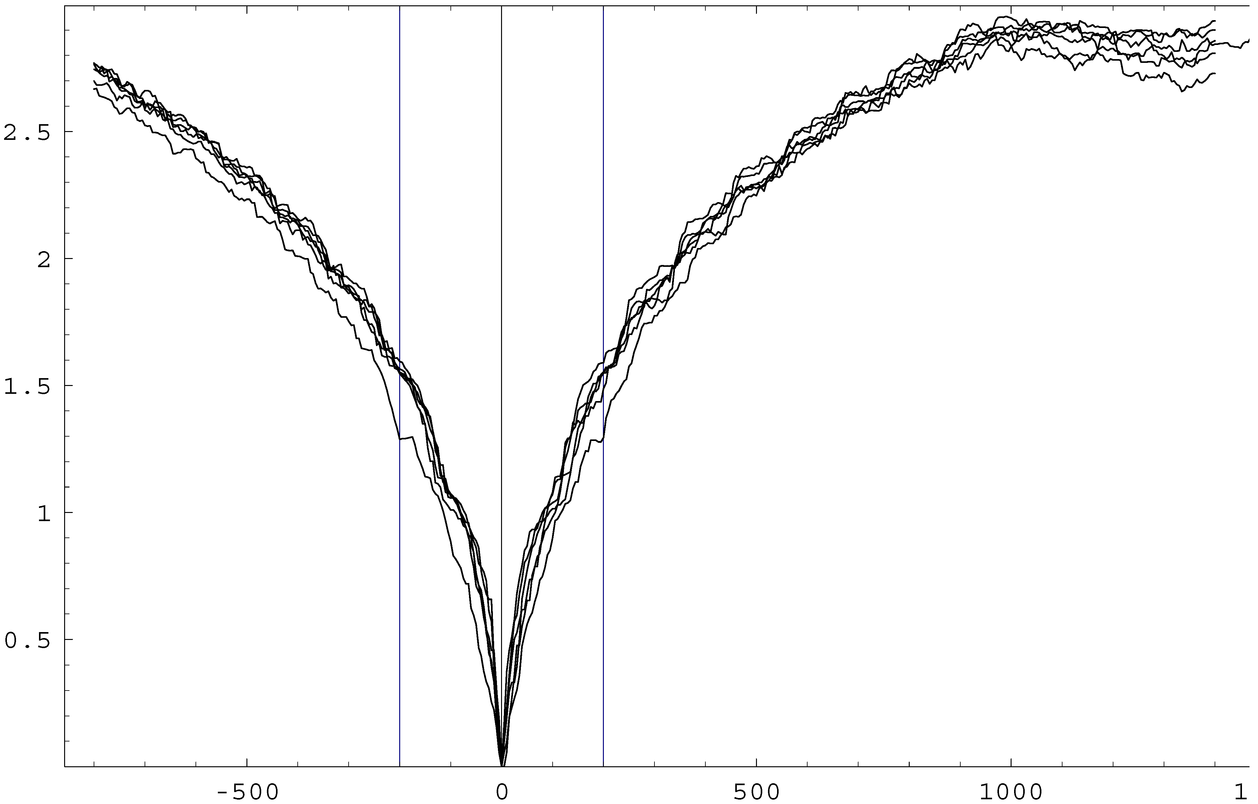
As another example, I calculated the effect on the solution in both directions of time that results from a microscopic perturbation of the state (in this case simply defined by an interchange of velocities between particles at some time t₀). Both boundary conditions are then violated by the new solution arising from this perturbed state, used as a complete “initial” condition. The results (shown in Fig. 2) are now most dramatic towards the former “past”, demonstrating the relevance of fine-grained information (similar to Borel’s example) for correctly calculating “backwards in time”. Deviations from the original two-time boundary solution close to t₀ also on the right are due to the fact that the coarse graining assumed in this model does not define a very good master equation (as discussed in [7]).

Figure 2. Time-symmetric “effect” on a solution “caused” by a perturbation of the microscopic state at time t₀ = 200, defined by an accidental entropy minimum at this time. The perturbed solution drastically violates both boundary conditions that were valid for the unperturbed solution.

Figure 2. Time-symmetric “effect” on a solution “caused” by a perturbation of the microscopic state at time t₀ = 200, defined by an accidental entropy minimum at this time. The perturbed solution drastically violates both boundary conditions that were valid for the unperturbed solution.

5 Cosmology and Gravitation

It appears evident from the above discussion that opposite arrows of time would in general require almost complete thermalization between initial and final conditions, which is hard to accomplish even in a cosmological setting. In its present stage, this universe is very far from equilibrium. A reversal of the thermodynamical arrow of time together with that of cosmic expansion, as suggested by Gold [12], would therefore require a total life time of the universe vastly larger than its present age. Weakly interacting fields may never thermodynamically “mix” with the rest of matter [13].

In particular, Davies and Twamley demonstrated [9] that an expanding and recontracting uni-verse would remain essentially transparent to electromagnetic waves between the two radiation eras. This means that advanced radiation resulting from all stars which will exist during the recontraction of our universe would be present now, apparently unrelated to any individual future sources because of their distance, but red- or blue-shifted, depending on the size of the universe at the time of (time-reversed) emission. According to Craig [10], this radiation would show up as a non-Planckian high-frequency tail of the cosmic background radiation resulting from the past ra-diation era (where it would be absorbed in time-reverse description). This leads to the consistency problems described in Sect.2.

While neutrinos from the future would presumably remain unobserved, gravity, despite its weak-ness, dominates the entropy capacity of this world, and leads to consequences which are the most difficult ones to reverse. Black holes are expected to harbor event horizons which would not be able ever to disappear in classical relativity, while in quantum field theory they are predicted to disappear into Hawking radiation in the distant future in an irreversible manner. However, contraction of gravitating objects, including the formation of black holes, requires that higher multipoles are radiated away. This radiation arrow is the basis of the “no hair theorem”, which would characterize the asymptotic final states of black holes in an asymptotically flat and time-directed universe. Because of the diverging time dilation close to a horizon, any coherent advanced radiation (with the future black hole as its retarded cause) would be able to arrive in time to pre-vent the formation of an horizon [14]. This solution of the “information loss paradox” may save a deterministic universe (without leading to inhomogeneous singularities).

While the required initial and final conditions are not obviously consistent in this classical scenario, this problem is relaxed in quantum cosmology.

6 Quantum Aspects

Realistic models of physical systems require quantum theory to be taken into account. Since quantum entropy is calculated from the density matrix (that may result from a wave function by means of generalized “coarse graining”), its time dependence has in principle to include a collapse of the wave function during measurements or other “measurement-like” situations (such as fluctuations or phase transitions). If the collapse represents a fundamental irreversible process, it defines an arrow of time that is never reversed. Only a universal Schrödinger equation (leading to an Everett interpretation) could be time (or CPT) symmetric. A reversal of the time arrow would then require decoherence to be replaced by recoherence: advanced Everett branches must combine with our world branch in order to produce local coherence. Although being far more complex than a classical model (since relying on those infamous “many worlds”) this would still allow us to conceive of a two-time boundary condition for a global wave function (see Sect. 4.6 of [7]). Note that Boltzmann’s statistical correlations (defined only for ensembles) now become quantum correlations (or entanglement, defined for individual quantum states). For example, re-expanding black holes, mentioned in the previous section, would in an essential way require (and possibly be facilitated by) recoherence.

In quantum gravity (or any other “reparametrization-invariant” theory), the Schrödinger equation is reduced to the Wheeler-DeWitt equation, HΨ = 0, which does not explicitly depend on time at all. However, because of its hyperbolic form, this equation defines an “intrinsic initial value problem” with respect to the expansion parameter a. In a classical (time-dependent) picture, the initial and final states would have to be identified in order to define one boundary condition, while the formal final condition (with respect to a) for recontracting universes is reduced to the usual normalizability of the wave function for a → ∞. Big bang and big crunch (distinguished by means of a WKB time, for example) could not even conceivably be different as (complete) quantum states (Chap. 6 of [7]), while forever expanding universes might be said to define an arrow of time that never changes direction during a WKB history. All arrows thus seem to be strongly entangled.

References

- Schulman, L.S. "Time’s arrows and quantum mechanics". Cambridge University Press, 1997. [Google Scholar]
- Schulman, L.S. Phys. Rev. Lett. 1999, 83, 5419.
- Schulman, L.S. "Time’s Arrow, Quantum Measurements and Superluminal Behavior". Mugnai, D., Ranfagni, A., Schulman, L.S., Eds.; Consiglio Nazionale delle Ricerche: Roma, 2001; – cond-mat/0102071. [Google Scholar]
- Wheeler, J.A.; Feynman, R.P. Rev. Mod. Phys. 1949, 21, 425.
- Lewis, D. Philosophical Papers. Vol. II, Oxford University Press, 1986. [Google Scholar]
- Price, H. "Time’s Arrow & Archimedes’ Point: A View from Nowhen". Oxford University Press, 1996. [Google Scholar]
- Zeh, H.D. "The Physical Basis of the Direction of Time". Springer: Berlin, 2001. [Google Scholar]
- Borel, E. "Le hasard". Alcan: Paris, 1924. [Google Scholar]
- Davies, P.C.W.; Twamley, J. Class. Quantum Grav. 1993, 10, 931. [CrossRef]
- Craig, D.A. Ann. Phys. (N.Y.) 1996, 251, 384.
- Kac, M. "Probability and Related Topics in Physical Sciences". Interscience, 1959. [Google Scholar]
- Gold, T. Am. J. Phys. 1962, 30, 403.
- Dyson, F. Phys. Rev. 1949, 75, 1736.
- Kiefer, C.; Zeh, H.D. Phys. Rev 1995, D51, 4145.
©2005 by MDPI (http://www.mdpi.org). Reproduction for noncommercial purposes permitted.
Share and Cite
MDPI and ACS Style
Zeh, H.D. Remarks on the Compatibility of Opposite Arrows of Time. Entropy 2005, 7, 199-207. https://doi.org/10.3390/e7040199
AMA Style
Zeh HD. Remarks on the Compatibility of Opposite Arrows of Time. Entropy. 2005; 7(4):199-207. https://doi.org/10.3390/e7040199
Chicago/Turabian StyleZeh, H. D. 2005. "Remarks on the Compatibility of Opposite Arrows of Time" Entropy 7, no. 4: 199-207. https://doi.org/10.3390/e7040199