Molecular Classification of Pesticides Including Persistent Organic Pollutants, Phenylurea and Sulphonylurea Herbicides

Abstract
:1. Introduction
2. Results and Discussion
MAPE = 5.39% AEV = 0.0234
MAPE = 5.84% AEV = 0.0214

| Compound | Rt (min) | Rt − Rt° (min) | (Rt − Rt°)/Rt° | logP | pKa | D | D’ |
|---|---|---|---|---|---|---|---|
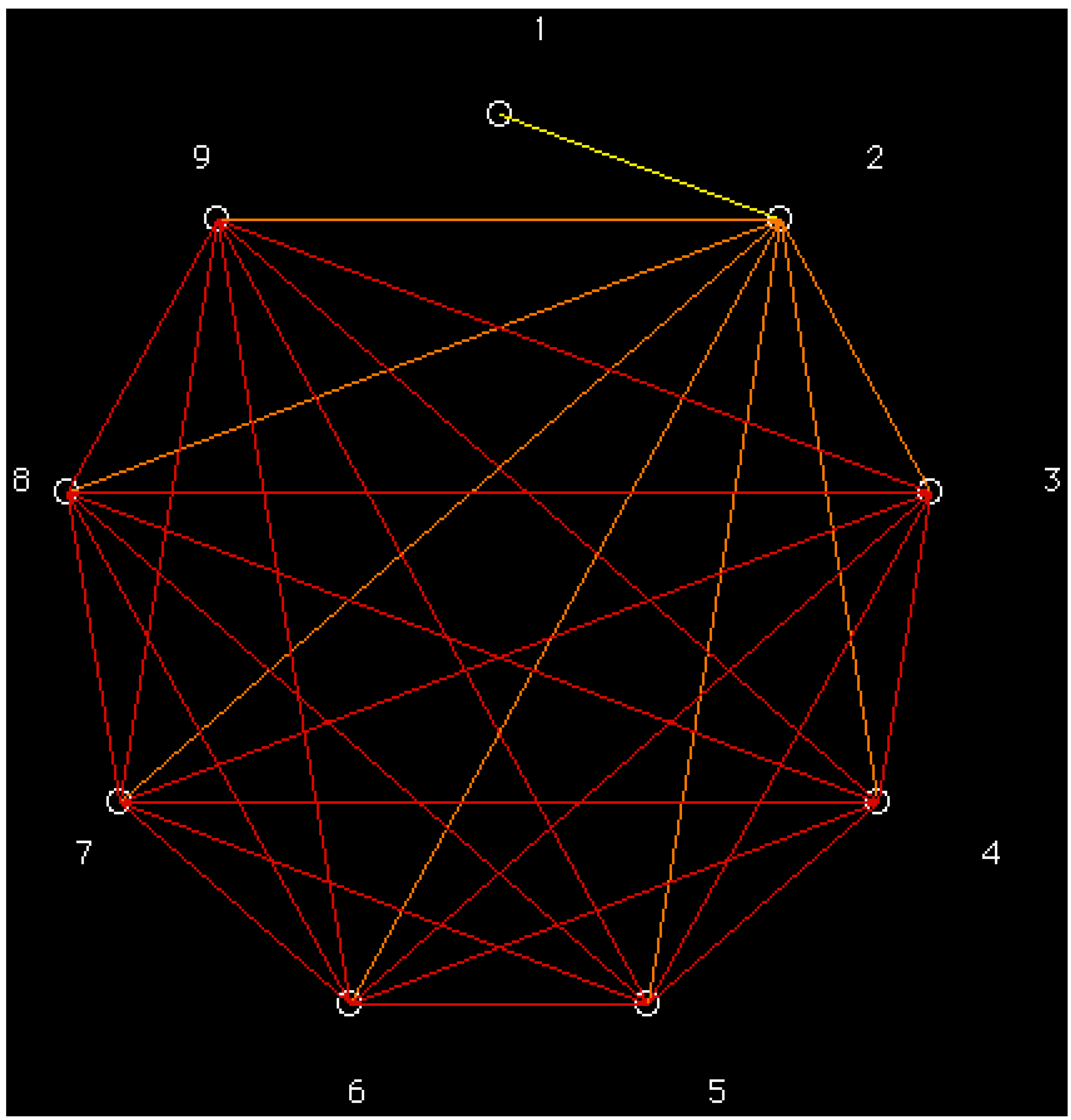
| 1. Methamidophos C2H8NO2PS <001010> | 2.78 | 0.00 | 0.00000 | −0.779 | −0.58 | 1.235 | 1.266 |
| 2. Carbendazim C9H9N3O2 <100010> | 6.48 | 3.70 | 1.33094 | 1.52 | 5.66 | 1.284 | 1.332 |
| 3. Thiabendazole C10H7N3S <110010> | 6.91 | 4.13 | 1.48561 | 2.47 | 3.40 | 1.288 | 1.331 |
| 4. Pyrimethanil C12H13N3 <110010> | 10.43 | 7.65 | 2.75180 | 2.558 | 4.41 | 1.314 | 1.407 |
| 5. Cyprodinil C14H15N3 <110010> | 11.44 | 8.66 | 3.11511 | 3.012 | 4.22 | 1.344 | 1.470 |
| 6. TPP (IS) C18H15O4P <111000> | 11.78 | 9.00 | 3.23741 | 4.63 | −5 | 1.394 | 1.504 |
| 7. Diazinone C12H21N2O3PS <111100> | 11.92 | 9.14 | 3.28777 | 3.766 | 1.21 | 1.398 | 1.509 |
| 8. Pyrazophos C14H20N3O5PS <111110> | 12.24 | 9.46 | 3.40288 | 2.810 | −1.37 | 1.403 | 1.505 |
| 9. Chlorpyrifos C9H11NO3PSCl3 <111111> | 13.42 | 10.64 | 3.82734 | 5.004 | −5.28 | 1.394 | 1.494 |


| Classification Level b | Number of Classes | Entropy h |
|---|---|---|
| 1.00 | 9 | 32.49 |
| 0.98 | 7 | 20.01 |
| 0.96 | 6 | 15.13 |
| 0.93 | 5 | 10.70 |
| 0.87 | 4 | 6.77 |
| 0.76 | 3 | 3.71 |
| 0.51 | 2 | 1.47 |
| 0.10 | 1 | 0.08 |


| Factor | Eigenvalue | Percentage of Variance | Cumulative Percentage of Variance |
|---|---|---|---|
| F1 | 2.33109829 | 38.85 | 38.85 |
| F2 | 1.62998318 | 27.17 | 66.02 |
| F3 | 1.25482746 | 20.91 | 86.93 |
| F4 | 0.38517751 | 6.42 | 93.35 |
| F5 | 0.33518718 | 5.59 | 98.94 |
| F6 | 0.06372637 | 1.06 | 100.00 |
| Property | PCA Factor Loadings a | |||||
|---|---|---|---|---|---|---|
| F1 | F2 | F3 | F4 | F1 | F6 | |
| i1 | 0.30822766 | 0.64474701 | 0.02673332 | −0.04594797 | 0.50138891 | −0.48485077 |
| i2 | 0.44804795 | 0.45046774 | −0.05731613 | 0.08927231 | −0.76002034 | 0.08629170 |
| i3 | 0.40956062 | −0.56947041 | −0.18574529 | 0.04102918 | −0.15327503 | −0.66954134 |
| i4 | 0.55772042 | −0.17916516 | 0.17892539 | 0.59525799 | 0.32511366 | 0.40595876 |
| i5 | −0.31588577 | 0.04253838 | 0.72852310 | 0.44514023 | −0.20425092 | −0.35748077 |
| i6 | 0.35450381 | −0.15222972 | 0.63145758 | −0.66011661 | 0.00822715 | 0.12881324 |
| Percentage of i1 a | % of i2 | % of i3 | % of i4 | % of i5 | % of i6 | |
|---|---|---|---|---|---|---|
| F1 | 9.50 | 20.07 | 16.77 | 31.11 | 9.98 | 12.57 |
| F2 | 41.57 | 20.29 | 32.43 | 3.21 | 0.18 | 2.32 |
| F3 | 0.07 | 0.33 | 3.45 | 3.20 | 53.07 | 39.87 |
| F4 | 0.21 | 0.80 | 0.17 | 35.43 | 19.81 | 43.58 |
| F5 | 25.14 | 57.76 | 2.35 | 10.57 | 4.17 | 0.01 |
| F6 | 23.51 | 0.74 | 44.83 | 16.48 | 12.78 | 1.66 |


| P. | g00100 | g00101 | g01100 | g10000 | g10001 | g10100 | g11000 | g11001 | g11100 | g11110 | g11111 |
|---|---|---|---|---|---|---|---|---|---|---|---|
| p0 | Chlordecone** | Methamidophos | PFOS** | Metamitron* BDE‑99** Metoxuron Monuron Diuron Linuron Buturon Chlorotoluron Daimuron Fenuron Methyldimuron Fluometuron Siduron Neburon Isoproturon Pencycuron | Carbendazim Metolachlor* Metazachlor | AMS BSM CME CNS EMS MSM NCS OXS PSE TFS TBM TFO 3FS RMS IDS | Carbetamide* Prometryne* Lindane** PCB** | Thiabendazole Pyrimethanil Cyprodinil Carbofuran* | TPP Flazasulphuron Triasulphuron Azimsulphuron Chlorsulphuron | Diazinone | Pyrazophos |
| p1 | Chlorfenvinphos** | Chlorpyrifos |

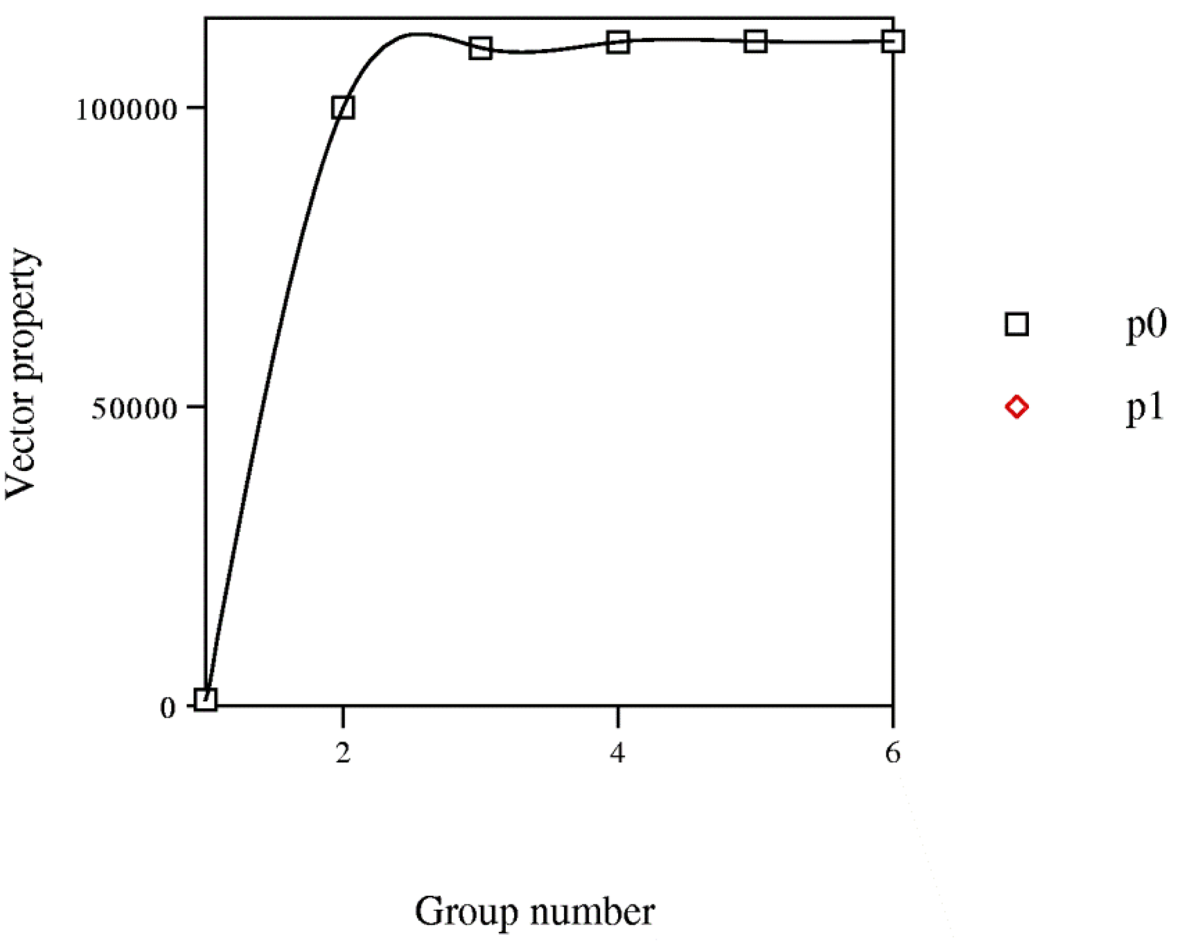
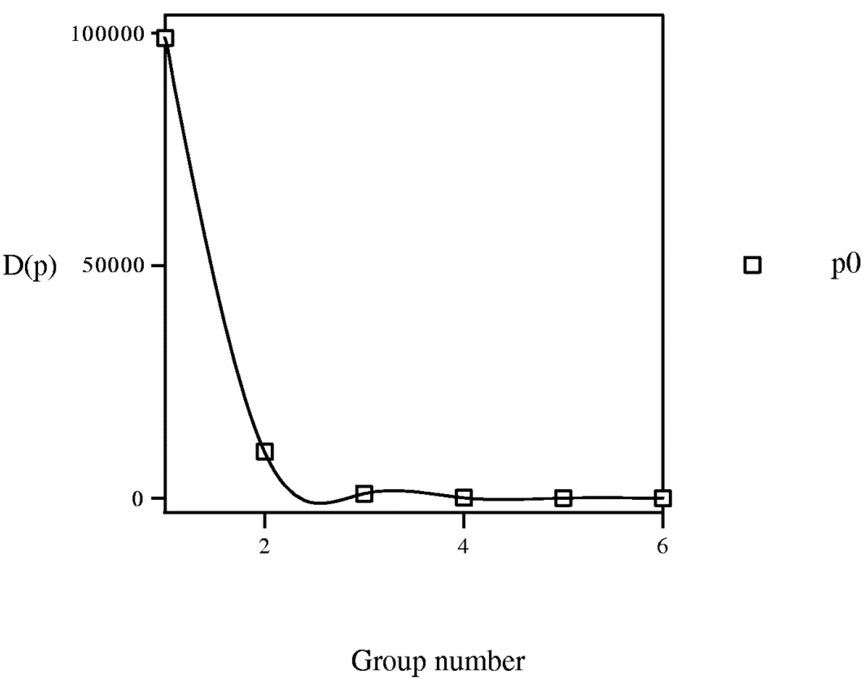
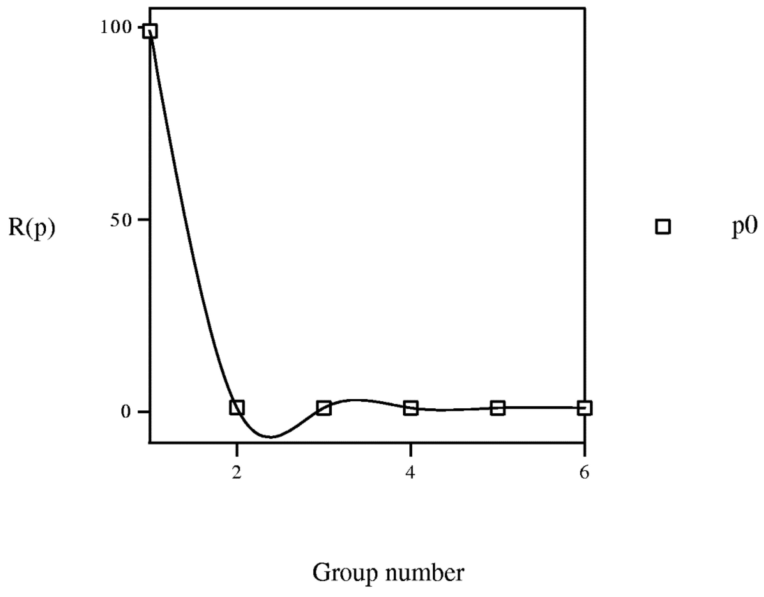
Pmin (P) < P(P+1)
P(P+1) − Pmin (P) >0


3. Experimental
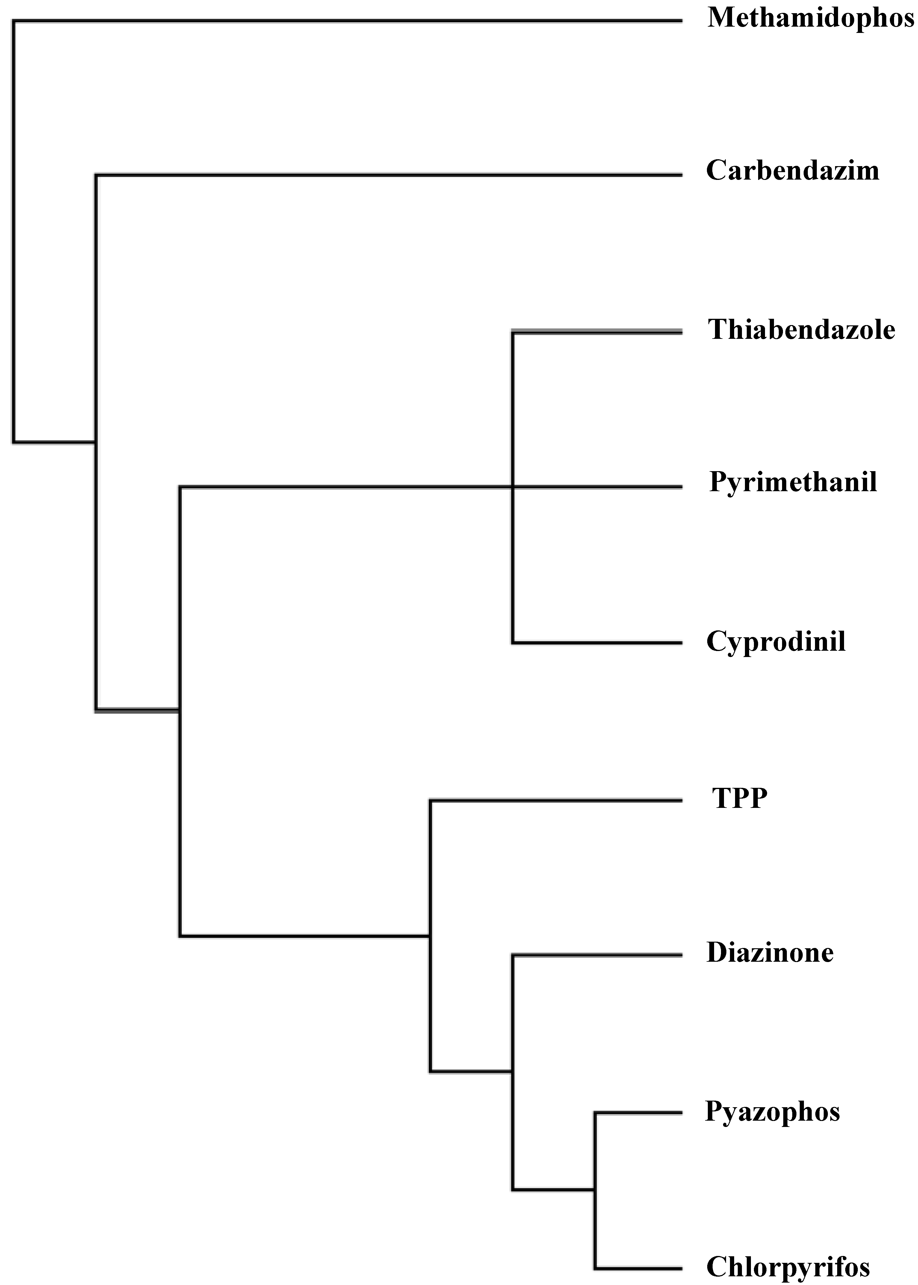
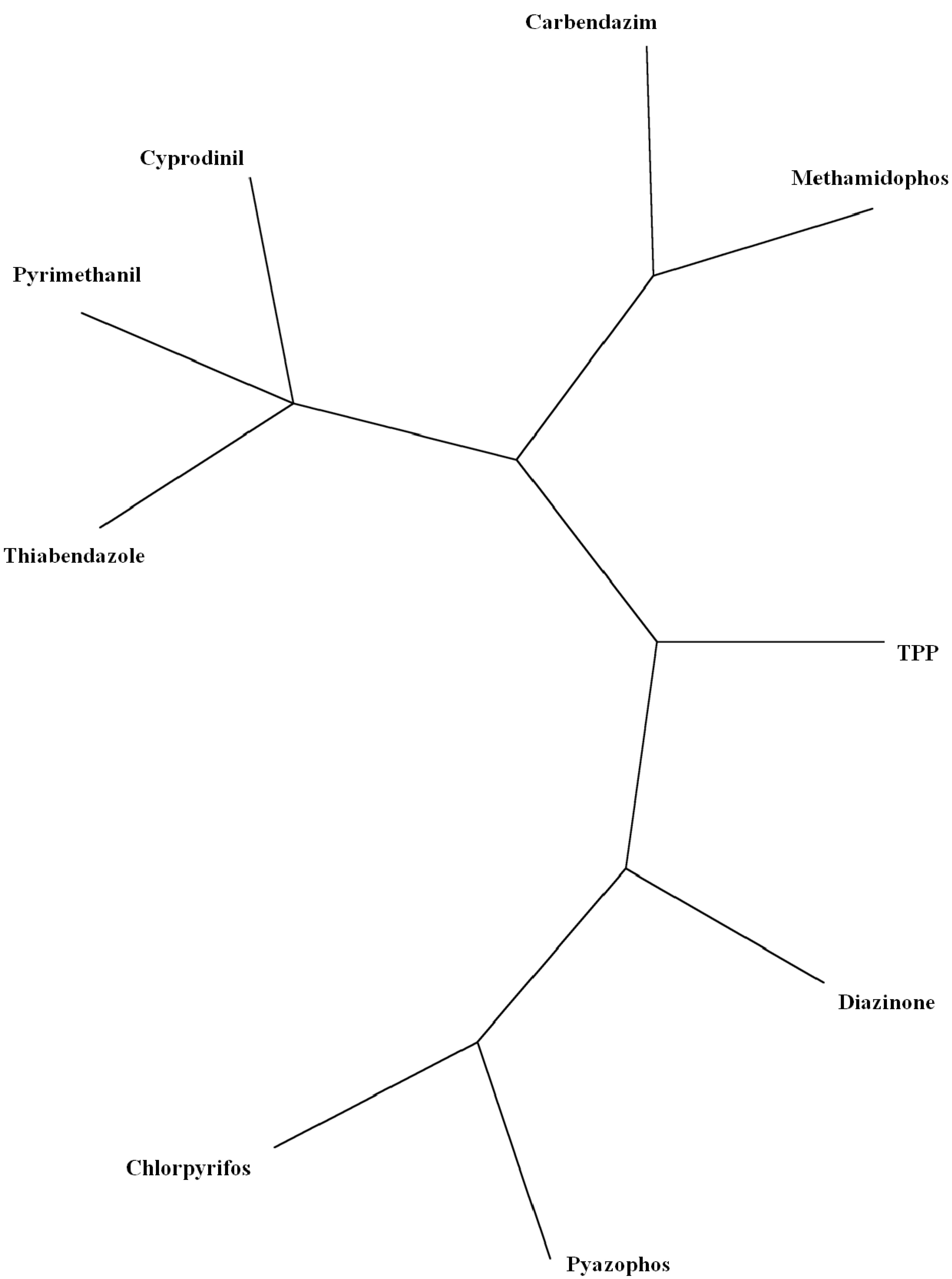
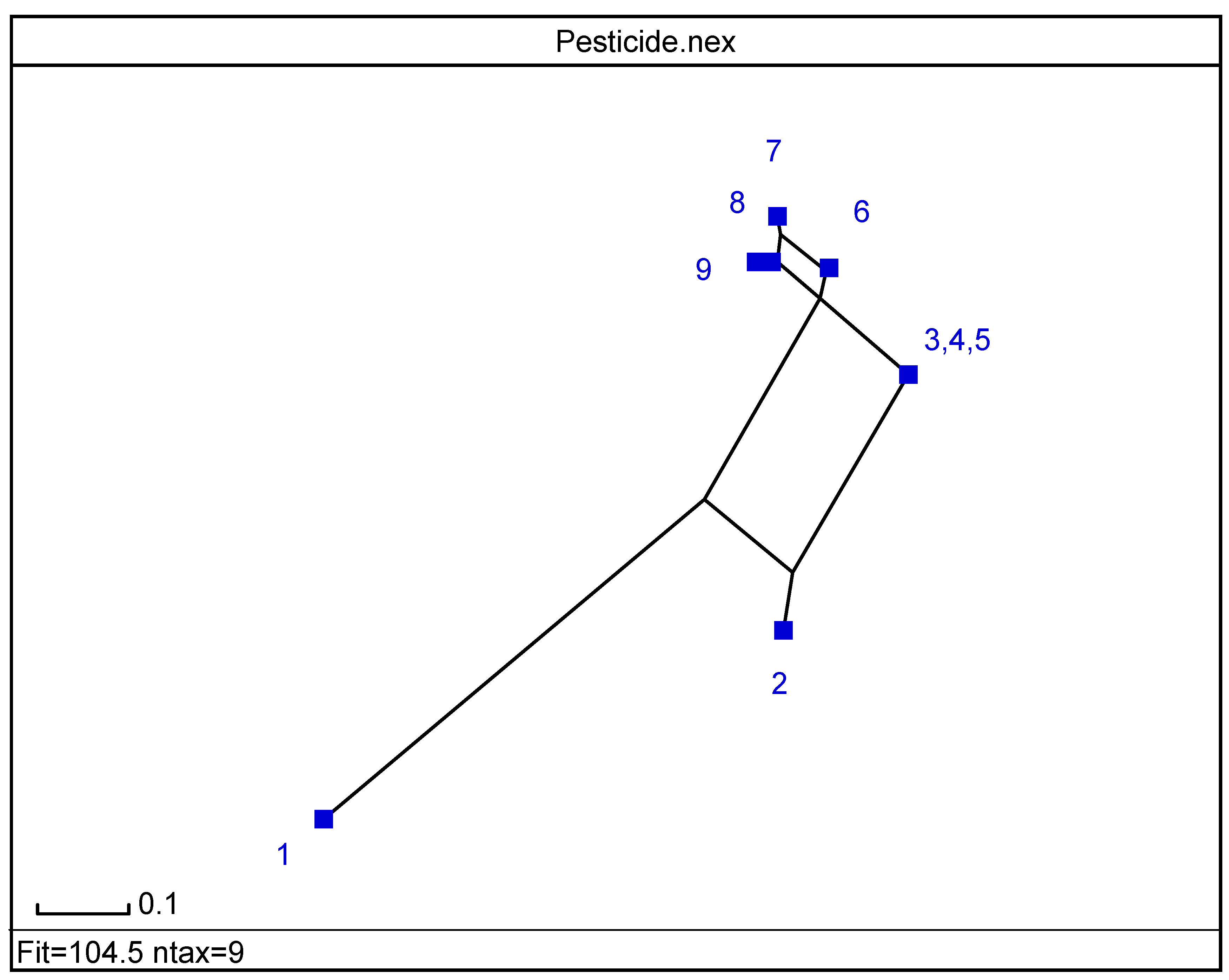
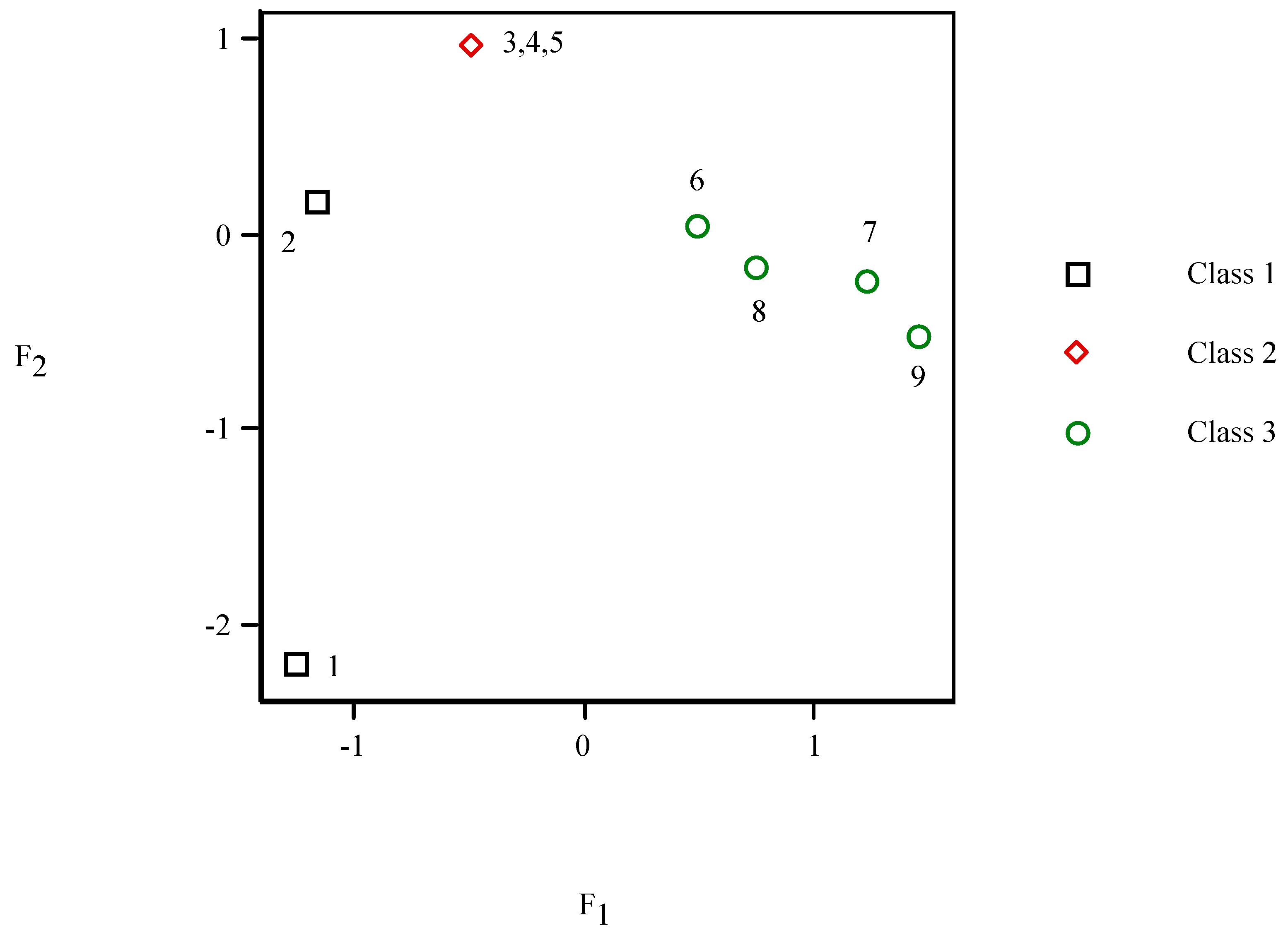
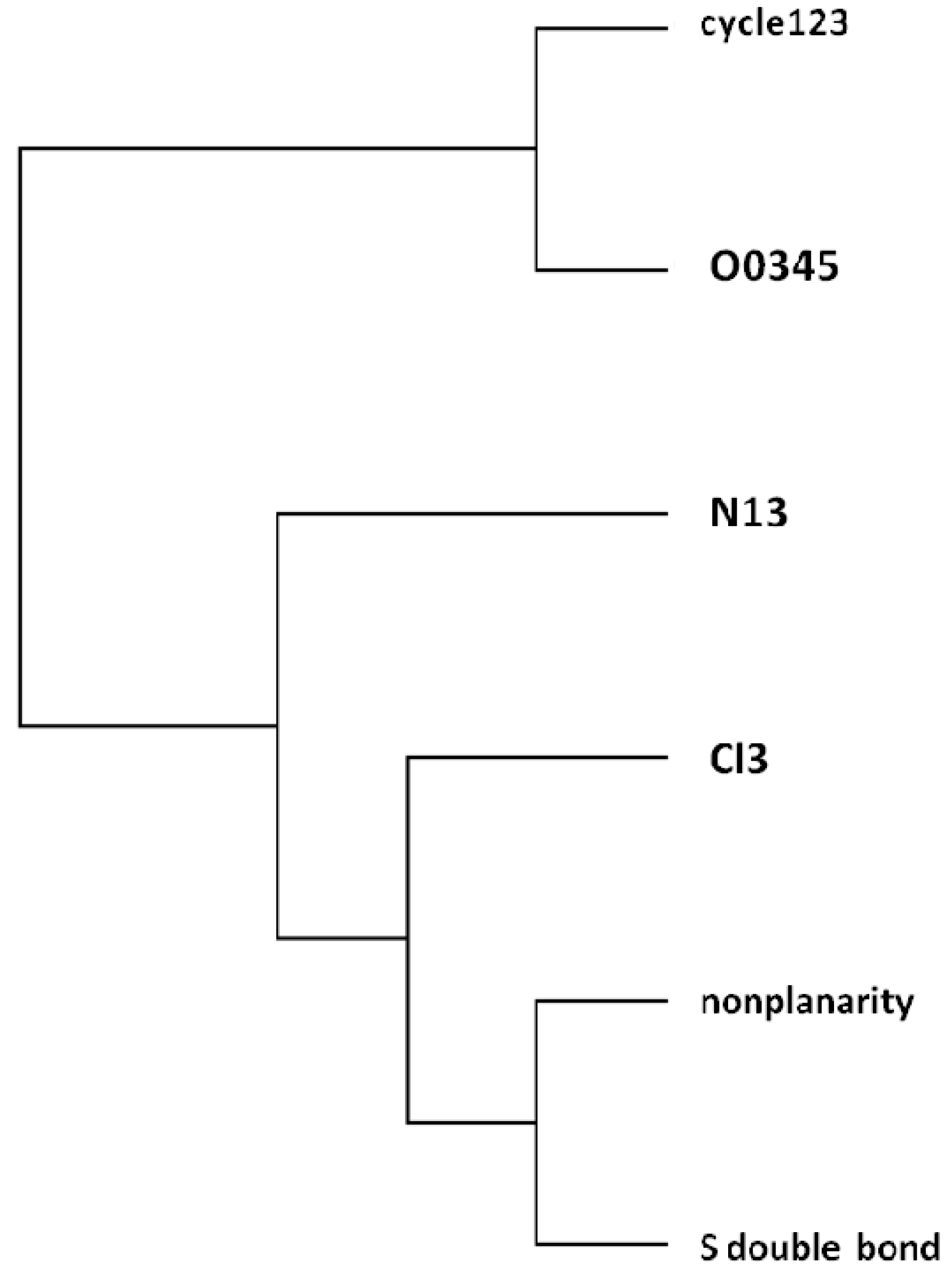
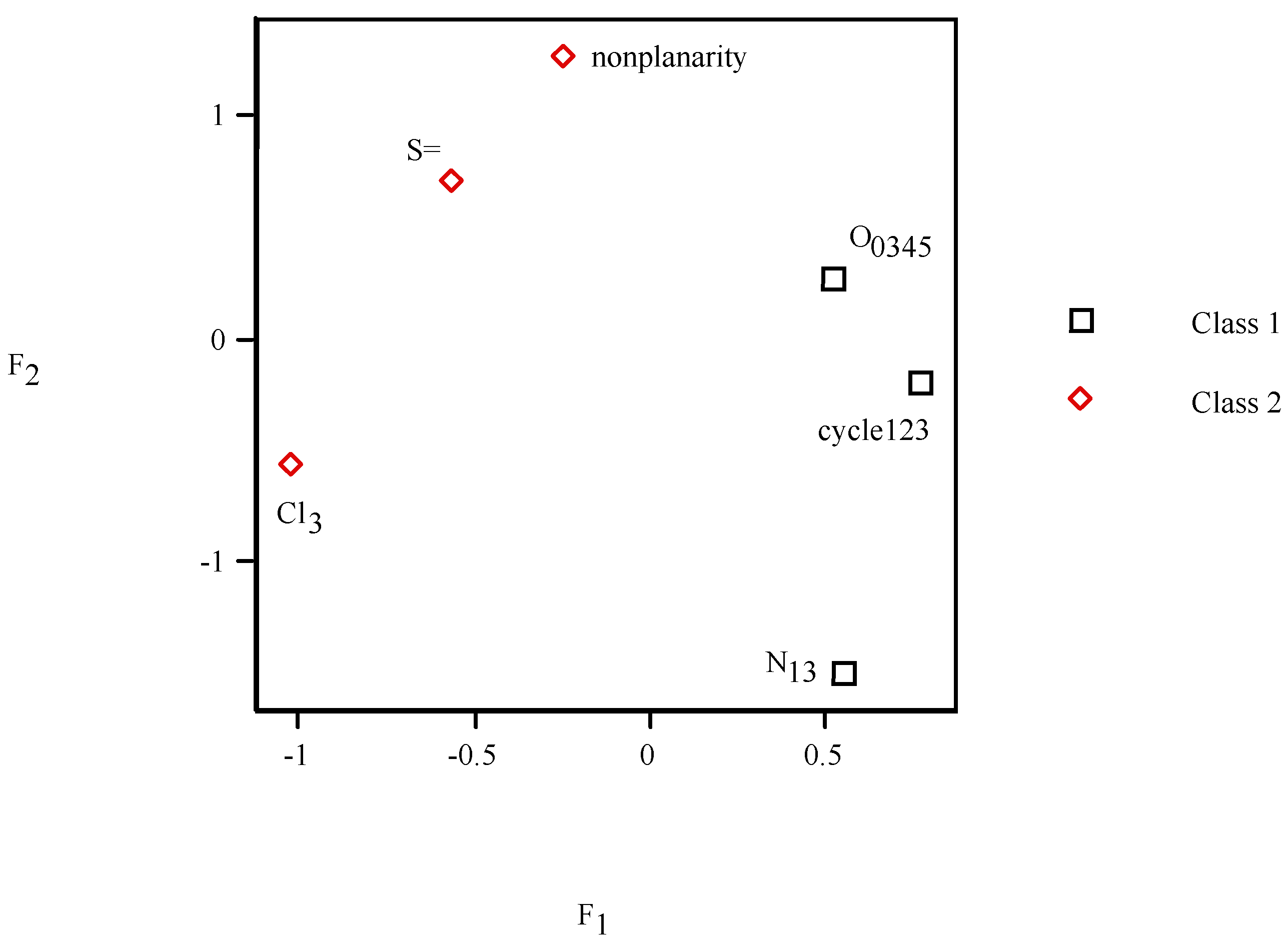
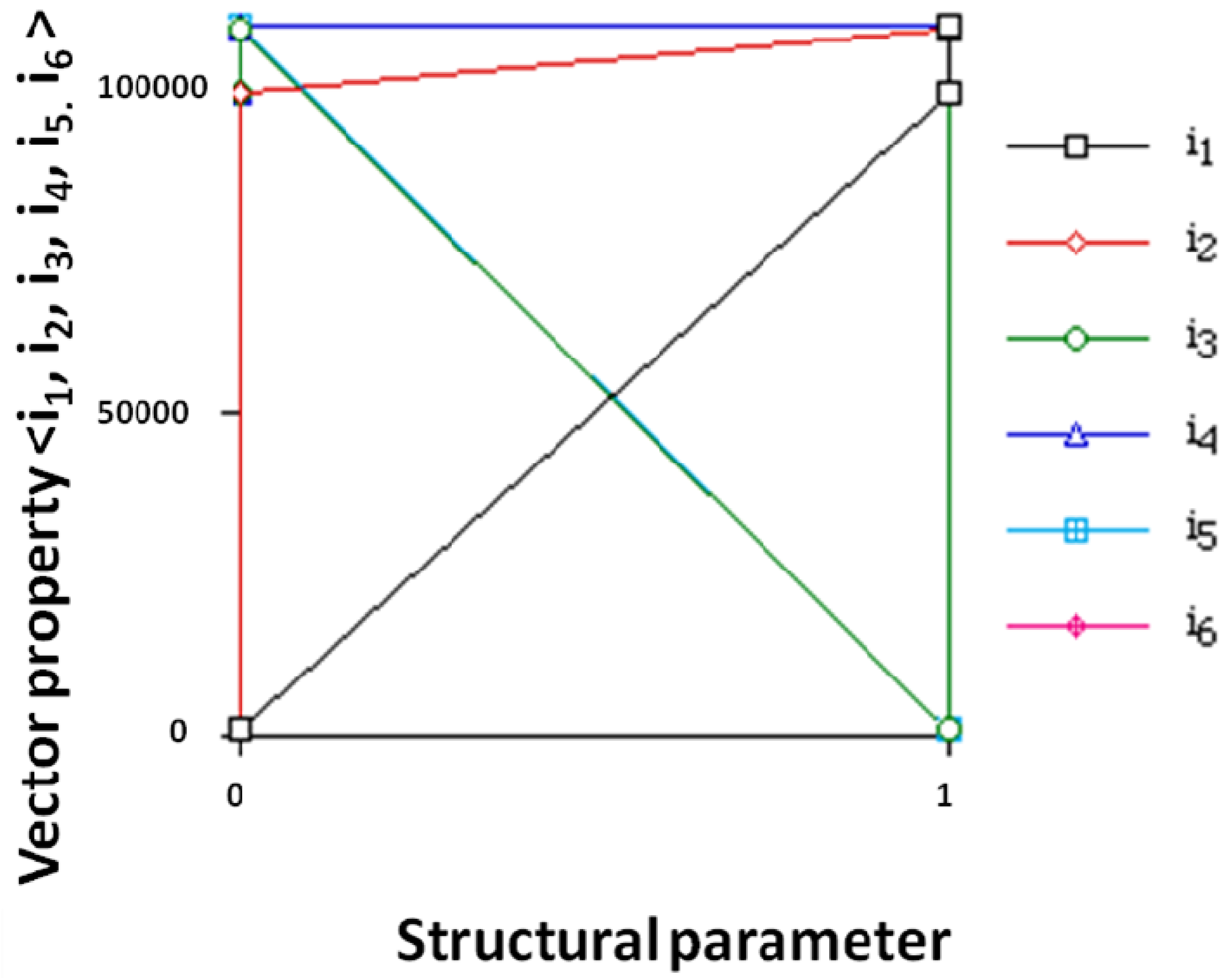
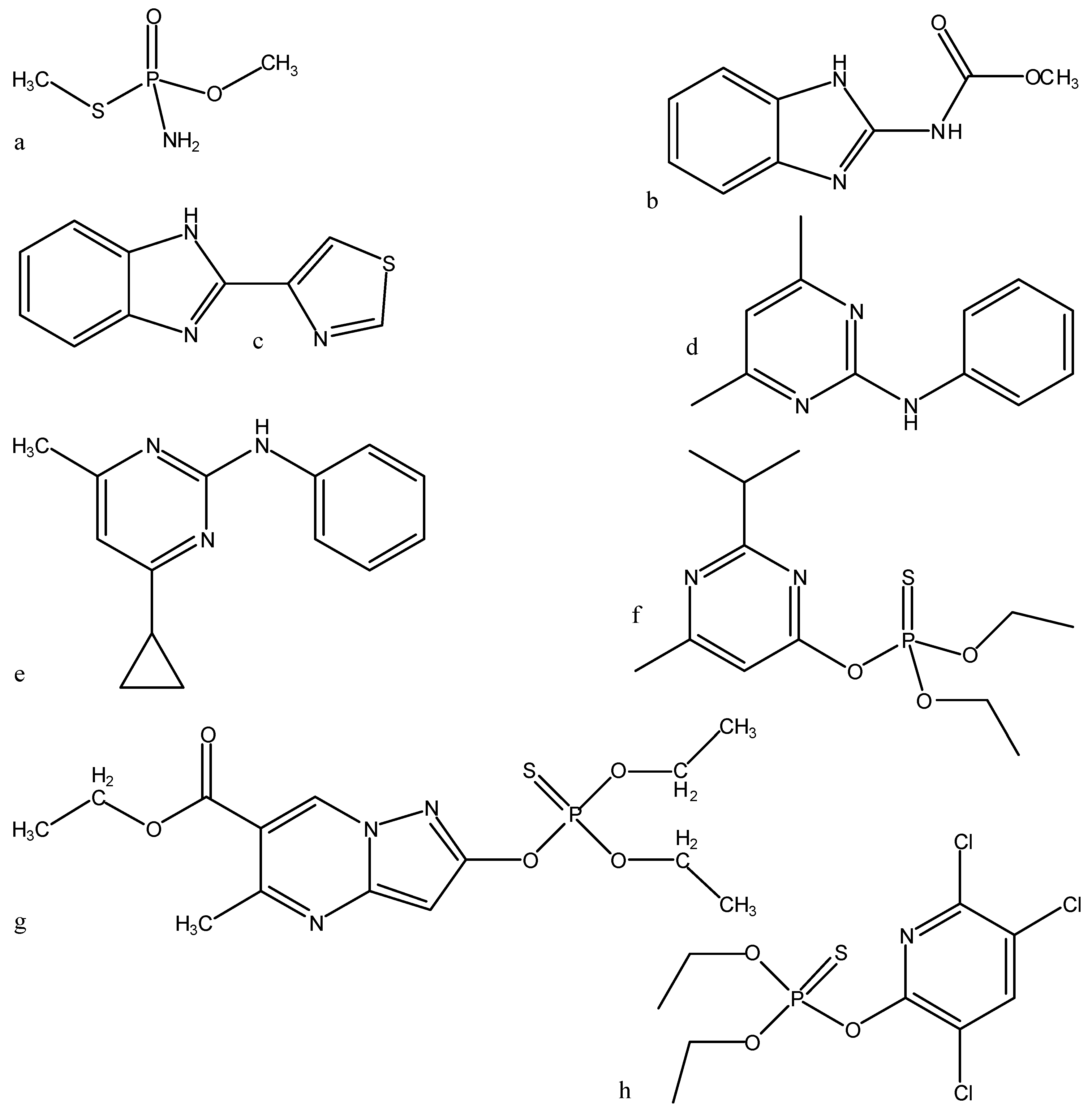
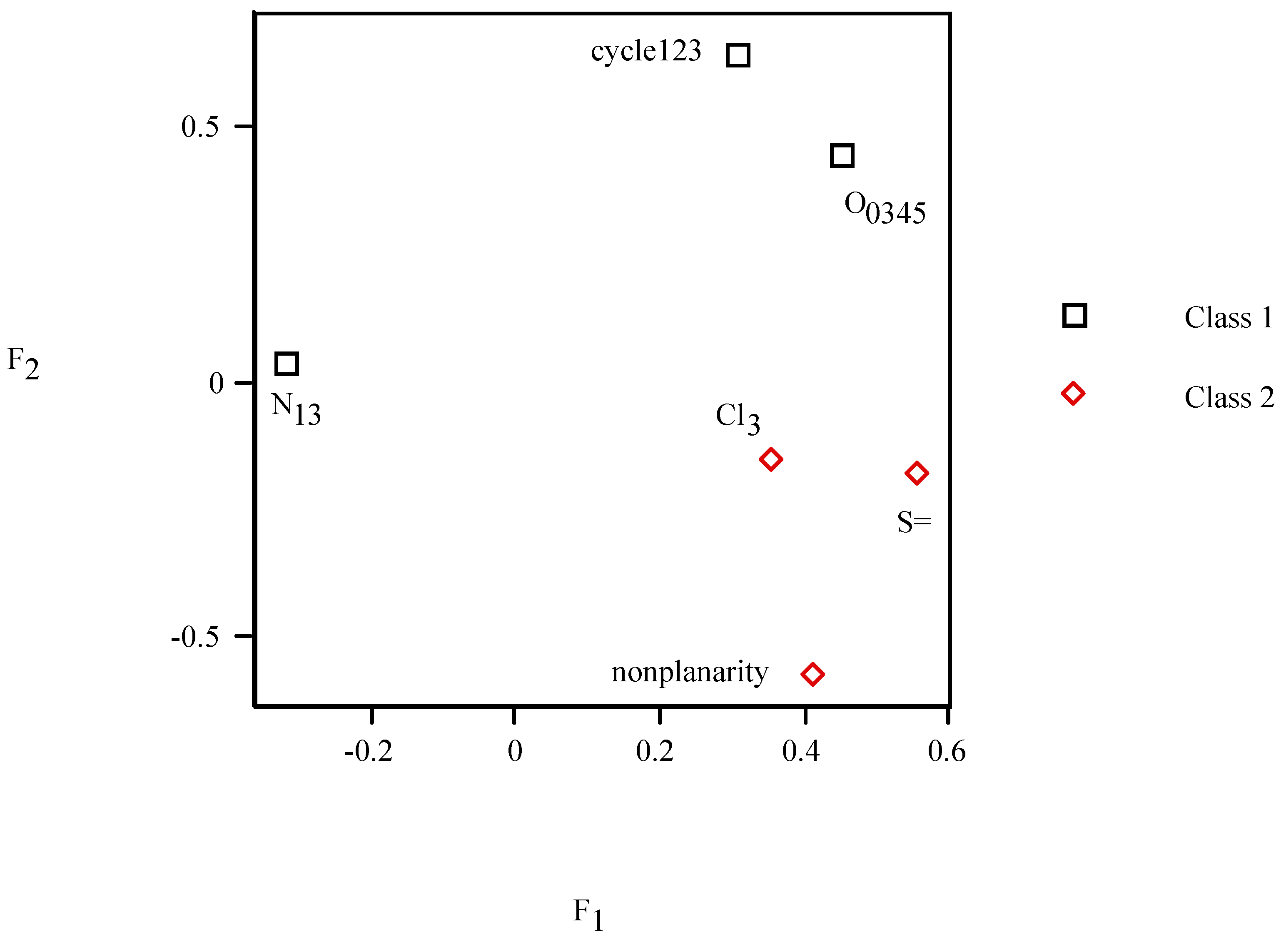
 = <i1,i2,…ik,…> should be associated with every pesticide i, whose components correspond to different molecular features in a hierarchical order according to their expected importance in retention. If characteristic m-th is chromatographically more significant for retention than k-th then m < k. Components ik are either “1” or “0”, according to whether a similar characteristic of rank k is either present or absent in pesticide i compared to a reference. Analysis includes six structural and constitutional characteristics: presence of cycle (cyc123), occurrence of either none or 3–5 O atoms (O0345), nonplanarity (NP), double-bonded S atom (S=), incidence of either one or three N atoms (N13) and existence of three Cl atoms (Cl3, cf. Figure 15). It is assumed that the chemical characteristics can be ranked according to their contribution to retention in the following order of decaying importance: cyc123 > O0345 > NP > S= > N13 > Cl3. Index i1 = 1 denotes cyc123 (i1 = 0 for cyc0), i2 = 1 means O0345 (i2 = 0 for O2), i3 = 1 signifies NP, i4 = 1 indicates S=, i5 = 1 stands for N13 (i5 = 0 for N0 or N2) and i6 = 1 represents Cl3 (i6 = 0 for Cl0). In chlorpyrifos number of cycles is one, O is three, it is NP and S=, number of N is one and number of Cl atoms is three; obviously its associated vector is <111111>. In this study chlorpyrifos was selected as reference because of its greatest retention. Table 1 contains vectors associated with nine pesticides. Vector <001010> is associated with methamidophos since it shows cyc0, O2, NP, not S=, N1 and Cl0. = <i1,i2,…ik…> and
  = <j1,j2,…jk…> is defined as:


3.1. Classification Algorithm
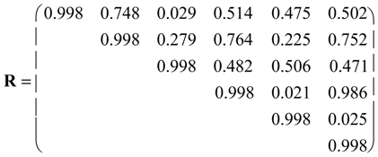
 is set of species j that satisfies rule: rij(n) ≥ b. Matrix of classes is:
 (similarly for t and
  ). Rule (13) means finding largest similarity index between species of two different classes.
3.2. Information Entropy

 similarity matrix at grouping level b. Information entropy satisfies following properties. (1) h(R) = 0 if either rij = 0 or rij = 1; (2) h(R) is maximum if rij = 0.5,i.e., when imprecision is maximum; (3) h( )≤h(R) for any b, i.e., classification leads to entropy loss; (4) h
  ≤h
≤h  if b1 < b2, i.e., entropy is monotone function of grouping level b.
3.3. Equipartition Conjecture of Entropy Production

3.4. Learning Procedure

4. Conclusions
- (1)
- The objective was to develop a structure–property relation for qualitative and quantitative prediction of chromatographic retention times of pesticides. Results of the present work contribute to relation prediction of pesticide residues, in food and environmental samples. Code TOPO allows fractal dimensions, and SCAP, solvation free energies and partition coefficient, which show that for a given atom energies and partitions are sensitive to the presence in the molecule of other atoms and functional groups. Fractal dimensions, partition coefficient, etc. differentiated pesticides. Parameters needed for co-ordination index are molar formation enthalpy, molecular weight and surface area. The morphological and co-ordination indices barely improved equations. Correlation between molecular area and weight points not only to a homogeneous molecular structure of pesticides, but also to the ability to predict and tailor their properties; the latter is nontrivial in environmental toxicology.
- (2)
- Several criteria selected to reduce the analysis to a manageable quantity of pesticides, referred to structural and constituent characteristics related to nonplanarity, and the number of rings, and O, double-bonded S, N and Cl atoms. Classification was in agreement with the principal component analyses. Program MolClas is a simple, reliable, efficient and fast procedure for molecular classification based on equipartition conjecture of entropy production. It was written to analyze equipartition conjecture of entropy production and explore molecular-classification world.
- (3)
- Periodic law does not satisfy physics-law status: (a) pesticides retentions are not repeated; perhaps chemical character; (b) order relations are repeated with exceptions. Analysis forces statement: Relations that any compound p has with its neighbour, p + 1, are approximately repeated for each period. Periodicity is not general; however, if substance natural order is accepted law must be phenomenological. Retention is not used in periodic-table generation and serves to validate it. The analysis of other properties would give an insight into the possible generality of the periodic table. The periodic classification was extended to phenylureas and sulphonylureas.
Acknowledgments
Author Contributions
Conflicts of Interest
References
- De Melo Abreu, S.; Caboni, P.; Cabras, P.; Garau, V.L.; Alves, A. Validation and global uncertainty of a liquid chromatographic with diode array detection method for the screening of azoxystrobin, kresoxim-methyl, trifloxystrobin, famoxadone, pyraclostrobin and fenamidone in grapes and wine. Anal. Chim. Acta 2006, 291, 573–574. [Google Scholar]
- Oliva, J.; Navarro, S.; Barba, A.; Navarro, G. Determination of chlorpyrifos, penconazole, fenarimol, vinclozolin and metalaxyl in grapes, must and wine by on-line microextraction and gas chromatography. J. Chromatogr. A 1999, 833, 43–51. [Google Scholar] [CrossRef]
- Jiménez, J.J.; Bernal, J.L.; del Nozal, M.J.; Toribio, L.; Arias, E. Analysis of pesticide residues in wine by solid-phase extraction and gas chromatography with electron capture and nitrogen–phosphorus detection. J. Chromatogr. A 2001, 919, 147–156. [Google Scholar] [CrossRef]
- Wang, J.F.; Luan, L.; Wang, Z.Q.; Jiang, S.R.; Pan, C.P. Determination of 19 multi-residue pesticides in grape wine by gas chromatography-mass spectrometry with micro liquid-liquid extraction and solid phase extraction. Chin. J. Anal. Chem. 2007, 35, 1430–1434. [Google Scholar]
- Economou, A.; Botitsi, H.; Antoniou, S.; Tsipi, D. Determination of multi-class pesticides in wines by solid-phase extraction and liquid chromatography-tandem mass spectrometry. J. Chromatogr. A 2009, 1216, 5856–5867. [Google Scholar] [CrossRef]
- Hu, Y.; Liu, W.M.; Zhou, Y.M.; Guan, Y.F. Determination of organophosphorous pesticide residues in red wine by solid phase microextraction-gas chromatography. Chin. J. Chromatogr. 2006, 24, 290–293. [Google Scholar]
- Wu, J.; Tragas, C.; Lord, H.; Pawliszyn, J. Analysis of polar pesticides in water and wine samples by automated in-tube solid-phase microextraction coupled with high-performance liquid chromatography–mass spectrometry. J. Chromatogr. A 2002, 976, 357–367. [Google Scholar] [CrossRef]
- Bolaños, P.P.; Romero-González, R.; Frenich, A.G.; Vidal, J.L.M. Application of hollow fibre liquid phase microextraction for the multiresidue determination of pesticides in alcoholic beverages by ultra-high pressure liquid chromatography coupled to tandem mass spectrometry. J. Chromatogr. A 2008, 1208, 16–24. [Google Scholar] [CrossRef]
- Vinas, P.; Aguinaga, N.; Campillo, N.; Hernández-Córdoba, M. Comparison of stir bar sorptive extraction and membrane-assisted solvent extraction for the ultra-performance liquid chromatographic determination of oxazole fungicide residues in wines and juices. J. Chromatogr. A 2008, 1194, 178–183. [Google Scholar] [CrossRef]
- Anastassiades, M.; Lehotay, S.J.; Stajnbaher, D.; Schenck, F.J. Fast and easy multiresidue method employing acetonitrile extraction/partitioning and “dispersive solid-phase extraction” for the determination of pesticide residues in produce. J. AOAC Int. 2003, 86, 412–431. [Google Scholar]
- Lehotay, S.J. Mass Spectrometry in Food Safety; Zweigenbaum, J., Ed.; Methods in Molecular Biology No. 747; Humana: Totowa, NJ, USA, 2011; pp. 65–91. [Google Scholar]
- Cunha, S.C.; Lehotay, S.J.; Mastovska, K.; Fernandes, J.O.; Beatriz, M.; Oliveira, P.P. Evaluation of the QuEChERS sample preparation approach for the analysis of pesticide residues in olives. J. Sep. Sci. 2007, 30, 620–632. [Google Scholar] [CrossRef]
- Whelan, M.; Kinsella, B.; Furey, A.; Moloney, M.; Cantwell, H.; Lehotay, S.J.; Danaher, M. Determination of anthelmintic drug residues in milk using ultra high performance liquid chromatography–tandem mass spectrometry with rapid polarity switching. J. Chromatogr. A 2010, 1217, 4612–4622. [Google Scholar] [CrossRef]
- Wang, X.; Telepchak, M.J. Determination of pesticides in red wine by QuEChERS extraction, rapid mini-cartridge cleanup and LC–MS–MS detection. LC·GC Eur. 2013, 26, 66–76. [Google Scholar]
- Blasco, C.; Picó, Y. Prospects for combining chemical and biological methods for integrated environmental assessment. Trends Anal. Chem. 2009, 28, 745–757. [Google Scholar] [CrossRef]
- de Umbuzeiro, A.G. (Ed.) Guia de Potabilidade para Substàncias Químicas. Limiar: São Paulo, Brazil, 2012. Available online: http://www.abes-sp.org.br/arquivos/ctsp/guia_potabilidade.pdf (accessed on 5 June 2014).
- Moganti, S.; Richardson, B.J.; McClellan, K.; Martin, M.; Lam, P.K.S.; Zheng, G.J. Use of the clam Asaphis deflorata as a potential indicator of organochlorine bioaccumulation in Hong Kong coastal sediments. Mar. Pollut. Bull. 2008, 57, 672–680. [Google Scholar] [CrossRef]
- Barco-Bonilla, N.; Romero-González, R.; Plaza-Bolaños, P.; Garrido Frenich, A.; Martínez Vidal, J.L. Analysis and study of the distribution of polar and non–polar pesticides in wastewater effluents from modern and conventional treatments. J. Chromatogr. A 2010, 1217, 7817–7825. [Google Scholar] [CrossRef]
- Navarro, A.; Tauler, R.; Lacorte, S.; Barceló, D. Chemometrical investigation of the presence and distribution of organochlorine and polyaromatic compounds in sediments of the Ebro River Basin. Anal. Bioanal. Chem. 2006, 385, 1020–1030. [Google Scholar] [CrossRef]
- Navarro-Ortega, A.; Tauler, R.; Lacorte, S.; Barceló, D. Occurrence and transport of PAHs, pesticides and alkylphenols in sediment samples along the Ebro River Basin. J. Hydrol. 2010, 383, 5–17. [Google Scholar] [CrossRef]
- Toropov, A.A.; Toropova, A.P.; Benfenati, E. QSPR modelling of the octanol/water partition coefficient of organometallic substances by optimal SMILES-based descriptors. Cent. Eur. J. Chem. 2009, 7, 846–856. [Google Scholar] [CrossRef]
- Toropova, A.P.; Toropov, A.A.; Benfenati, E.; Gini, G. QSAR models for toxicity of organic substances to Daphnia magna built up by using the CORAL freeware. Chem. Biol. Drug Des. 2011, 79, 332–338. [Google Scholar]
- Toropov, A.A.; Toropova, A.P. Optimal descriptor as a translator of eclectic data into endpoint prediction: Mutagenicity of fullerene as a mathematical function of conditions. Chemosphere 2014, 104, 262–264. [Google Scholar] [CrossRef]
- Kar, S.; Roy, K. Predictive chemometric modeling and three-dimensional toxicophore mapping of diverse organic chemicals causing bioluminescent repression of the bacterium genus Pseudomonas. Ind. Eng. Chem. Res. 2013, 52, 17648–17657. [Google Scholar] [CrossRef]
- Roy, K.; Das, R.N.; Popelier, P.L.A. Quantitative structure–activity relationship for toxicity of ionic liquids to Daphnia magna: Aromaticity vs. lipophilicity. Chemosphere 2014, 112, 120–127. [Google Scholar] [CrossRef]
- Torrens, F. Free energy of solvation and partition coefficients in methanol–water binary mixtures. Chromatographia 2001, 53, S199–S203. [Google Scholar] [CrossRef]
- Soria, V.; Campos, A.; Figueruelo, J.E.; Gómez, C.; Porcar, I.; García, R. Modelling of stationary phase in size-exclusion chromatography with binary eluents. In Strategies in Size Exclusion Chromatography; Potschka, M., Dubin, P.L., Eds.; ACS Symposium Series. No. 635; American Chemical Society: Washington, DC, USA, 1996; Volume Cnapter 7, pp. 103–126. [Google Scholar]
- Torrens, F.; Soria, V. Stationary-mobile phase distribution coefficient for polystyrene standards. Sep. Sci. Technol. 2002, 37, 1653–1665. [Google Scholar] [CrossRef]
- Torrens, F. A new chemical index inspired by biological plastic evolution. Indian J. Chem. Sect. A 2003, 42, 1258–1263. [Google Scholar]
- Torrens, F. A chemical index inspired by biological plastic evolution: Valence-isoelectronic series of aromatics. J. Chem. Inf. Comput. Sci. 2004, 44, 575–581. [Google Scholar] [CrossRef]
- Torrens, F.; Castellano, G. QSPR prediction of retention times of phenylurea herbicides by biological plastic evolution. Curr. Drug Saf. 2012, 7, 262–268. [Google Scholar] [CrossRef]
- Torrens, F.; Castellano, G. Molecular categorization of phenylurea and sulphonylurea herbicides, pesticides and persistent organic pollutants. In QSAR in Drug and Environmental Research; Roy, K., Ed.; IGI Global: Hershey, PA, USA, 2015; in press.
- Torrens, F.; Castellano, G. QSPR prediction of chromatographic retention times of pesticides: Partition and fractal indices. J. Environ. Sci. Health Part B 2014, 49, 400–407. [Google Scholar] [CrossRef]
- Varmuza, K. Pattern Recognition in Chemistry; Springer: New York, NY, USA, 1980. [Google Scholar]
- Benzecri, J.P. L’Analyse des Données; Dunod: Paris, France, 1984; volume 1. [Google Scholar]
- Tondeur, D.; Kvaalen, E. Equipartition of entropy production. An optimality criterion for transfer and separation processes. Ind. Eng. Chem. Fundam. 1987, 26, 50–56. [Google Scholar] [CrossRef]
- Torrens, F. Characterizing cavity-like spaces in active-site models of zeolites. Comput. Mater. Sci. 2003, 27, 96–101. [Google Scholar] [CrossRef]
- IMSL. In Integrated Mathematical Statistical Library (IMSL); IMSL: Houston, TX, USA, 1989.
- Tryon, R.C. A multivariate analysis of the risk of coronary heart disease in Framingham. J. Chronic Dis. 1939, 20, 511–524. [Google Scholar]
- Jarvis, R.A.; Patrick, E.A. Clustering using a similarity measure based on shared nearest neighbors. IEEE Trans. Comput. 1973, C22, 1025–1034. [Google Scholar] [CrossRef]
- Page, R.D.M. Program TreeView; Universiy of Glasgow: Glasgow, UK, 2000. [Google Scholar]
- Huson, D.H. SplitsTree: Analizing and visualizing evolutionary data. Bioinformatics 1998, 14, 68–73. [Google Scholar] [CrossRef]
- Hotelling, H. Analysis of a complex of statistical variables into principal components. J. Educ. Psychol. 1933, 24, 417–441. [Google Scholar] [CrossRef]
- Kramer, R. Chemometric Techniques for Quantitative Analysis; Marcel Dekker: New York, NY, USA, 1998. [Google Scholar]
- Patra, S.K.; Mandal, A.K.; Pal, M.K. State of aggregation of bilirubin in aqueous solution: Principal component analysis approach. J. Photochem. Photobiol. A 1999, 122, 23–31. [Google Scholar] [CrossRef]
- Jolliffe, I.T. Principal Component Analysis; Springer: Berlin, Germany, 2002. [Google Scholar]
- Xu, J.; Hagler, A. Chemoinformatics and drug discovery. Molecules 2002, 7, 566–600. [Google Scholar] [CrossRef]
- Shaw, P.J.A. Multivariate Statistics for the Environmental Sciences; Hodder-Arnold: New York, NY, USA, 2003. [Google Scholar]
- Kaur, M.; Malik, A.K.; Singh, B. Determination of phenylurea herbicides in tap water and soft drink samples by HPLC–UV and solid-phase extraction. LC·GC Eur. 2013, 25, 120–129. [Google Scholar]
- Can, A.; Yildiz, I.; Guvendik, G. The determination of toxicities of sulphonylurea and phenylurea herbicides with quantitative structure–toxicity relationship (QSTR) studies. Environ. Toxicol. Pharmacol. 2013, 35, 369–379. [Google Scholar] [CrossRef]
- Cabrera, K.; Altmaier, S. High-resolution and ultra trace analysis of pesticides using silica monoliths. Int. Labmate 2013, 38, 4–5. [Google Scholar]
- Forster, S.; Altmaier, S. Qualitative LC–MS analysis of pesticides using monolithic silica capillaries and potential for assay of pesticides in kidney. LC·GC Eur. 2013, 26, 488–496. [Google Scholar]
- Nold, M. Analytical standards for persistent organic pollutants. Analytix 2009, 2009, 11–12. [Google Scholar]
- Kaufmann, A. Introduction à la Théorie des Sous-ensembles Flous; Masson: Paris, France, 1975; volume 3. [Google Scholar]
- Cox, E. The Fuzzy Systems Handbook; Academic: New York, NY, USA, 1994. [Google Scholar]
- Kundu, S. The min–max composition rule and its superiority over the usual max–min composition rule. Fuzzy Sets Sys. 1998, 93, 319–329. [Google Scholar] [CrossRef]
- Lambert-Torres, G.; Pereira Pinto, J.O.; Borges da Silva, L.E. Minmax techniques. In Wiley Encyclopedia of Electrical and Electronics Engineering; Wiley: New York, NY, USA, 1999. [Google Scholar]
- Shannon, C.E. A mathematical theory of communication: Part I, discrete noiseless systems. Bell Syst. Tech. J. 1948, 27, 379–423. [Google Scholar] [CrossRef]
- Shannon, C.E. A mathematical theory of communication: Part II, the discrete channel with noise. Bell Syst. Tech. J. 1948, 27, 623–656. [Google Scholar] [CrossRef]
- White, H. Neural network learning and statistics. AI Expert 1989, 4, 48–52. [Google Scholar]
- Kullback, S. Information Theory and Statistics; Wiley: New York, NY, USA, 1959. [Google Scholar]
- Iordache, O.; Corriou, J.P.; Garrido-Sánchez, L.; Fonteix, C.; Tondeur, D. Neural network frames. application to biochemical kinetic diagnosis. Comput. Chem. Eng. 1993, 17, 1101–1113. [Google Scholar] [CrossRef]
- Iordache, O. Modeling Multi-Level Systems; Springer: Berlin, Germany, 2011. [Google Scholar]
- Iordache, O. Self-Evolvable Systems: Machine Learning in Social Media; Springer: Berlin, Germany, 2012. [Google Scholar]
- Iordache, O. Polytope Projects; CRC: Boca Raton, FL, USA, 2014. [Google Scholar]
- Sample Availability: Not available.
© 2014 by the authors. licensee MDPI, Basel, Switzerland. This article is an open access article distributed under the terms and conditions of the Creative Commons Attribution license ( http://creativecommons.org/licenses/by/3.0/).
Share and Cite
Torrens, F.; Castellano, G. Molecular Classification of Pesticides Including Persistent Organic Pollutants, Phenylurea and Sulphonylurea Herbicides. Molecules 2014, 19, 7388-7414. https://doi.org/10.3390/molecules19067388
Torrens F, Castellano G. Molecular Classification of Pesticides Including Persistent Organic Pollutants, Phenylurea and Sulphonylurea Herbicides. Molecules. 2014; 19(6):7388-7414. https://doi.org/10.3390/molecules19067388
Chicago/Turabian StyleTorrens, Francisco, and Gloria Castellano. 2014. "Molecular Classification of Pesticides Including Persistent Organic Pollutants, Phenylurea and Sulphonylurea Herbicides" Molecules 19, no. 6: 7388-7414. https://doi.org/10.3390/molecules19067388