Photobleaching Kinetics and Time-Integrated Emission of Fluorescent Probes in Cellular Membranes

Abstract
:1. Introduction
2. Results and Discussion
2.1. Limits of Fluorescence as Measure of Probe Concentration

 is a geometric factor related to the collection efficiency of the optical system with θ being the local convergence angle of the illumination/collecting beam at the sample plane (i.e., fluorescence microscopy is a form of reflected light microscopy, where the objective plays also the role of the condenser). The wavelength-dependent quantum yield of the detector is
  , while
  denotes the quantum yield of the fluorophore. The excitation intensity is Iex and is given in W/cm2. Using the relation 1 W = 1 J/s, it follows that Iex, sometimes also named irradiance, is equivalently given in J/(s cm2). It can be also expressed as photon flux with units photons/(s cm2) by using the energy of illumination photons of a given wavelength, i.e.,
  with Planck’s constant as h = 6.626 × 10⁻³⁴ J∙s and the speed of light as c = 300,000 km/s = 3 × 10¹⁷ nm/s [39]. This would give, for example, for a wavelength of λ = 320 nm, as used for excitation of DHE, E = 6.211 × 10⁻¹⁹ J per photon. Accordingly, an excitation energy of 1 W/cm2 = 1 J/(s∙cm2) corresponds to 1.61 × 10¹⁸ photons/(s∙cm2). Similarly, for blue photons with λ = 500 nm, as used for excitation of BChol, 1 W/cm2 corresponds to 2.515 × 10¹⁸ photons/(s∙cm2). In Equation (1), ε is the molar extinction coefficient (in M−1 cm−1), b is the optical path length (in cm) and c, is the probe concentration (in M). This equation, though central for our purpose, assumes fluorescence being linearly related to excitation energy. It is therefore strictly valid only for highly diluted solutions, in which fluorophores do not interact and for low irradiation, where fluorophores do not saturate. Thus, Equation (1) does not tell about the limitations of fluorescence detection for measurement of probe concentration, namely fluorescence quenching, saturation and photobleaching. To understand these processes, it is very instructive to start with some photokinetic considerations.


 , with
  being the illumination intensity (as irradiance in W/cm2 or as photon flux in photons/(s∙cm2), see above, and
  is the absorption cross-section of the fluorophore (in cm2 per molecule) for the given wavelength of excitation. The absorption cross-section is related to the extinction coefficient as
  , where NA is Avogadro’s number (6.0221 × 10²³ mol−1). Thus, k1 is for each molecule given in W = J/s, or equivalently, if the energy of illumination photons of a given wavelength is considered (as described above), in photons/s [39]. The measurable fluorescence lifetime,
  , is the reciprocal of the rate constant k−1 and comprises radiative and non-radiative deexcitation. The solution of this system can be easily found by standard methods and reads for S1(t) for the initial conditions S0(t = 0) = M (the number of illuminated molecules) and S1(t = 0) = 0, see Equation (5):

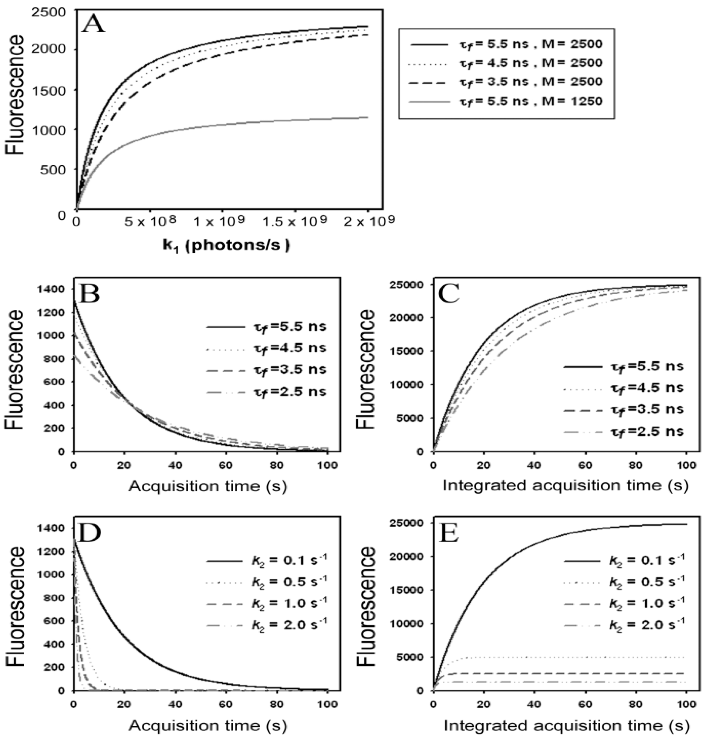
 ) as function of excitation intensity, one finds a saturation curve, where for increasing intensity, Iex, the plot deviates from a linear relationship (Figure 1A). Here, we used the mean fluorescence lifetime of BChol, a recently introduced fluorescent analog of cholesterol, as measured in model membranes [41] and in cells (i.e., τf ~5.5 ns) [26]. Accordingly, one needs to set the excitation energy and acquisition time as short as possible for obtaining good signal-to-noise ratios with maximal detector sensitivity.
 , the extinction coefficient was set to the value of BChol (1.32842 × 10⁻¹⁶ cm2). The number of fluorophores is given by M, while the fluorescent lifetime is τf = 1/k−1 (in ns); (B) simulation of photobleaching using Equation (10), as function of the fluorescence lifetime (values are indicated in the panel) for a fixed excitation rate constant of
  2 × 10⁵ photons/s and bleach rate constant
  0.1 s−1, and M = 2500; (C) simulation of fluorescence as function of integrated acquisition time using Equation (14) and same parameters as in panel B. The influence of the intrinsic bleach rate constant, k2, on photobleaching kinetics (D) and integrated fluorescence (E) is simulated according to Equations (13) and (14), respectively, using a fluorescence lifetime of τf = 5.5 ns,
  2 × 10⁵ photons/s and M = 2,500. See text for further explanations.
, the extinction coefficient was set to the value of BChol (1.32842 × 10⁻¹⁶ cm2). The number of fluorophores is given by M, while the fluorescent lifetime is τf = 1/k−1 (in ns); (B) simulation of photobleaching using Equation (10), as function of the fluorescence lifetime (values are indicated in the panel) for a fixed excitation rate constant of 2 × 10⁵ photons/s and bleach rate constant 0.1 s−1, and M = 2500; (C) simulation of fluorescence as function of integrated acquisition time using Equation (14) and same parameters as in panel B. The influence of the intrinsic bleach rate constant, k2, on photobleaching kinetics (D) and integrated fluorescence (E) is simulated according to Equations (13) and (14), respectively, using a fluorescence lifetime of τf = 5.5 ns, 2 × 10⁵ photons/s and M = 2,500. See text for further explanations.
2 × 10⁵ photons/s and M = 2,500. See text for further explanations.
, the extinction coefficient was set to the value of BChol (1.32842 × 10⁻¹⁶ cm2). The number of fluorophores is given by M, while the fluorescent lifetime is τf = 1/k−1 (in ns); (B) simulation of photobleaching using Equation (10), as function of the fluorescence lifetime (values are indicated in the panel) for a fixed excitation rate constant of 2 × 10⁵ photons/s and bleach rate constant 0.1 s−1, and M = 2500; (C) simulation of fluorescence as function of integrated acquisition time using Equation (14) and same parameters as in panel B. The influence of the intrinsic bleach rate constant, k2, on photobleaching kinetics (D) and integrated fluorescence (E) is simulated according to Equations (13) and (14), respectively, using a fluorescence lifetime of τf = 5.5 ns, 2 × 10⁵ photons/s and M = 2,500. See text for further explanations.
2.2. A Simple Model for Photobleaching and Time-Integrated Emission


 as well as the observed photobleaching rate constant
  of a fluorophore will be lowered in the presence of a collisional quencher due to an effective decrease of q (Figure 1B).
  , and phenomenological photobleaching rate constant,
  , show saturation behavior for high values of q (in photons/molecule), which can, for example, simulate increasing illumination intensity (not shown, but see [46]). Such saturation of fluorescence and bleach rate constant as function of illumination has been measured for the BODIPY and rhodamine fluorophore [47,48]. A static quencher will only lower the number of fluorophores participating in the photocycle, i.e., M in the model, but not the photobleaching kinetics (not shown). In general, any differences in fluorescence lifetime caused by locally varying fluorescence quantum yield in the cellular environment should be ‘detectable’ as a small change in photobleaching rate constant, as illustrated in Figure 1B. This effect has been used in the so-called donor photobleaching method for detecting Förster resonance energy transfer between fluorophore couples [49,50,51]. Since image acquisition requires integration of the fluorescence signal over some time period, varying the fluorescence lifetime for a given intrinsic photobleaching rate constant (e.g., k2 = 0.1 s−1) could affect the detected intensity, even in the first acquired frame. To test this in more detail, we calculate the time integral, F, for Equation (14) giving Equation (15):


 , the TiEm from the excited singlet state. Reasons for variation of the intrinsic bleach rate constant can be manifold. For example, in cell membranes k2 could vary due to different availability of molecular oxygen for photooxidation. Differences in detected TiEm due to variation of the intrinsic photobleaching rate constant, k2, can thus become very large, since for lower values of k2, it requires longer illumination and more photocycles to totally bleach the pool of available fluorophores (Figure 1E). In other words, the total fluorescence being collectable from a given number of fluorophores before the whole population is bleached depends on intrinsic properties of the probe, like its intrinsic bleach rate constant, k2, but not on the fluorescence lifetime, τf, as first shown in an elegant study by Hirschfeld [35], and reconciled here (compare Figure 1C,E).
  , since he included the dye-specific radiative lifetime as proportionality constant (see Equation (9) in [35]). Finally, the simple model of Equations (14) and (15) allows for deriving the TiEm solely from the acquired bleach curve. Let’s assume one performs a non-linear regression of a mono-exponential decay function of the form
  to a measured bleach curve recorded for a fluorophore in cells. Here, the bleach time constant determined by the fit is τ = 1/kb, and B is a measure of the background autofluorescence (assumed to bleach very slowly, see [36,52]). The decay amplitude, A, again, can be associated with the initial intensity of Equation (14), i.e.,
  . Direct integration of this mono-exponential decay function results in a linear term B·t in the time integral, such that the estimated TiEm would be compromised by autofluorescence (see Supplemental Information and discussion in [36]). With the model in Equation (14) and by having
  , we get the TiEm of Equation (16) simply as the product of A and τ, thereby automatically correcting for autofluorescence!
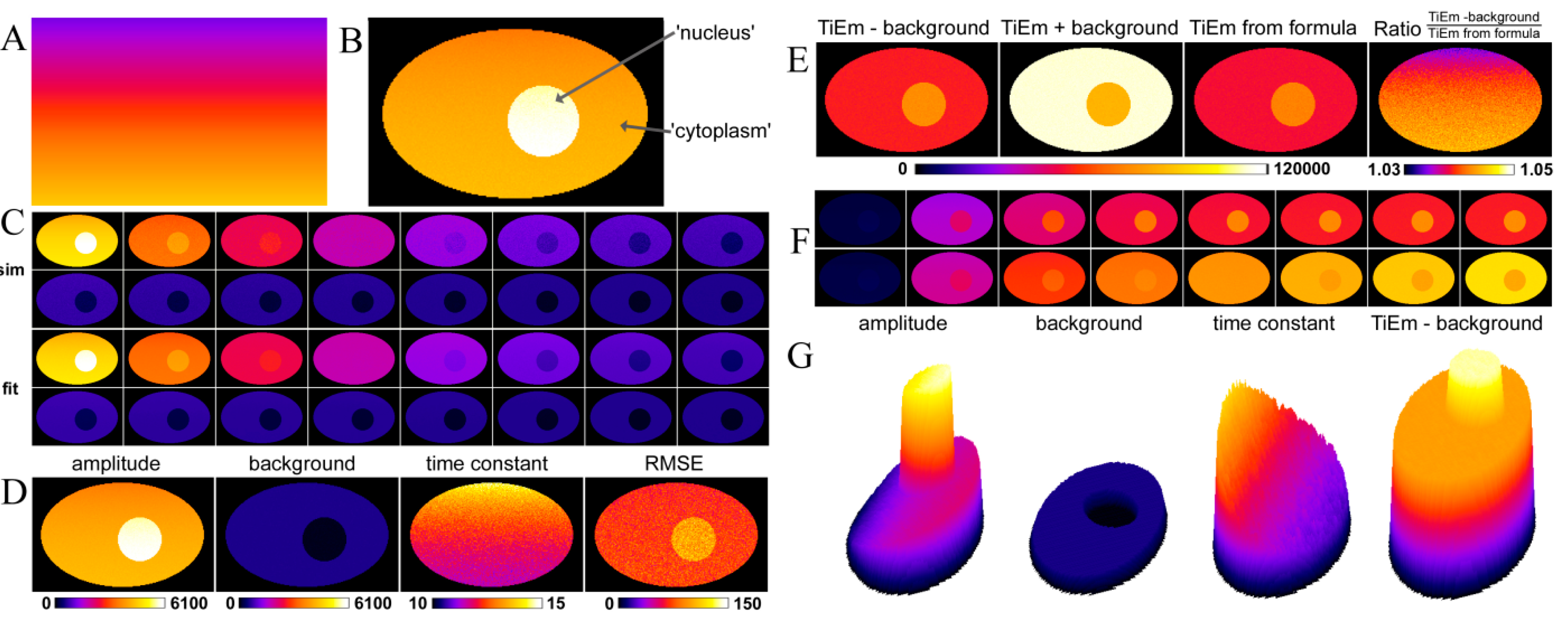
2.3. Validation of the Model Using Synthetic Fluorescence Images


2.4. Validation of the Model Using Live-Cell Images of Dehydroergosterol-Labeled Fibroblasts

2.5. Analysis of Photobleaching and Time-Integrated Emission in the Presence of a Triplet State


 , it follows directly from the Rough-Hurwitz criterion that
  and
and  . The corresponding eigenvectors and thereby the solution of Equations (20) and (21) can be also calculated but give formidably complex expressions (not shown). The presence of two different eigenvalues results in a bi-exponential bleaching decay with dependencies on all involved rate constants. Accordingly, also the interpretation of TiEm in the presence of a triplet state,
  , will be less straightforward than in the case of bleaching from a singlet state only. The only remaining feature is that
  remains, as
  , proportional to the number of fluorophores, M. Accordingly, in both cases, presence of static fluorophore quenching by complex formation would lower the TiEm proportionally and independent of the actual bleaching kinetics. Bi-exponential photobleaching due to photoreaction from the triplet state has been observed for fluorescein [60,61].


 in photons/molecule. Using the initial condition
  and Equations (31)–(33), above, we obtain Equation (35):


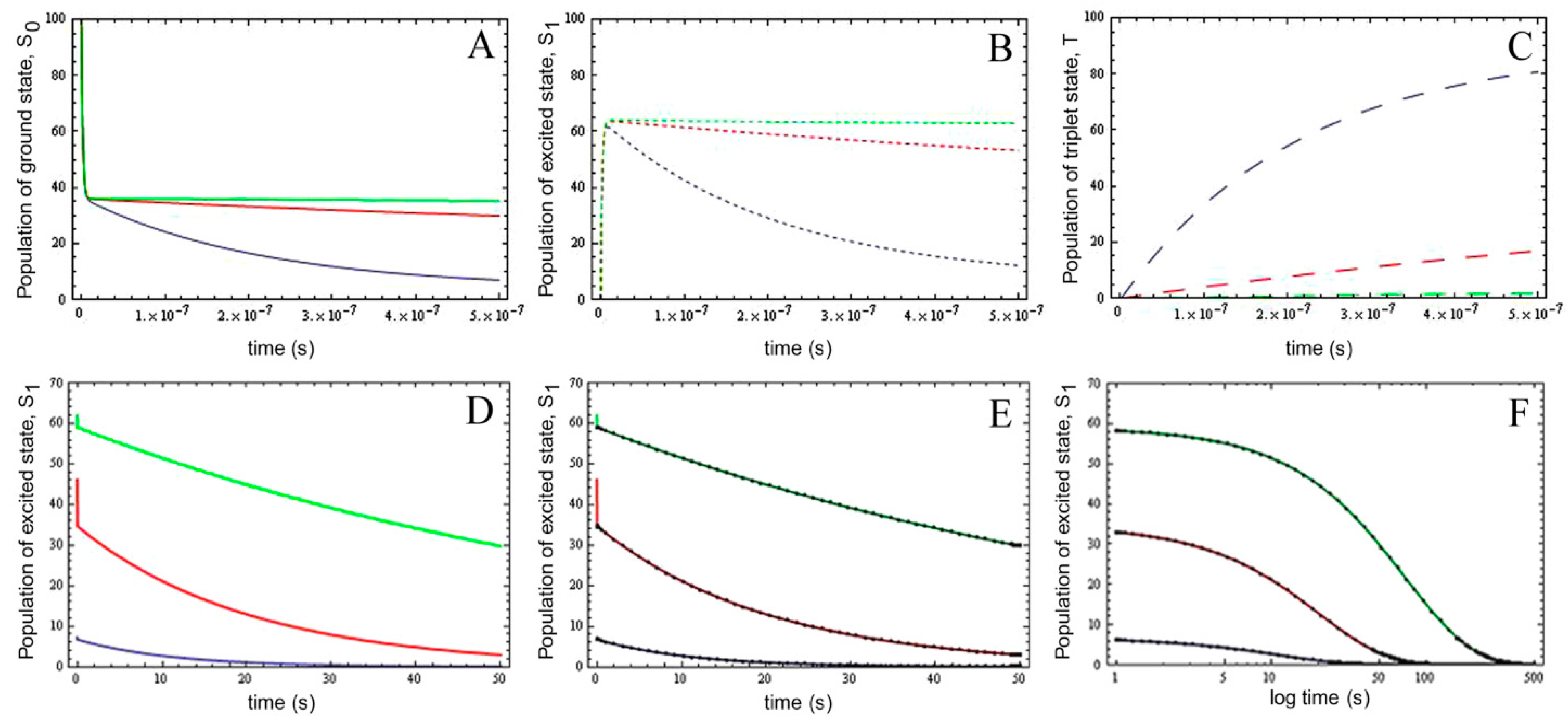
 = 660/50 = 13.2, cyan line;
  = 66/5 = 13.2, pink line and
  = 6.6/0.5 = 13.2, blue line). In fact, when the intersystem crossing rate constant is only 66fold higher than the bleach rate constant from the triplet state, the analytical model misses more than the first sec of observed photobleaching (see Supporting figure, blue line). In other words, when significant bleaching takes place BEFORE the equilibration of the electronic states on the first two time scales (see above), our model cannot describe the photobleaching dynamics. Thus, fluorophores bleaching preferentially from the triplet state but having very low spin-orbit coupling in a given environment cannot be studied with our photobleaching model. The model outlined in Equations (20) to (27), in which the triplet state dynamics is explicitly taken into account would account for this situation.
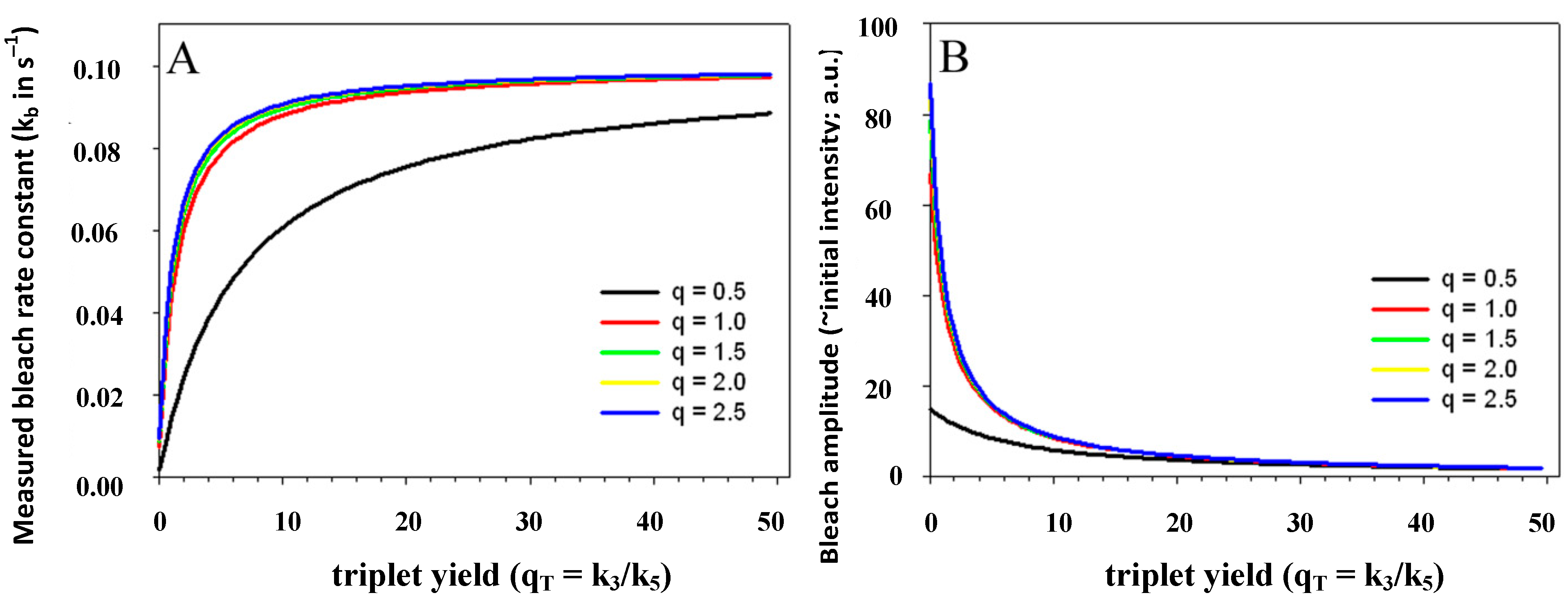
  ) is known to vary significantly not only between different fluorophores, but also in different environments. This has been shown, for example, for fluorescein in water versus ethanol [59]. As shown in Figure 5 in a simulation using the analytical bleaching model of Equation (35), the triplet yield has a profound effect on the bleaching amplitude,
  , and on the empirical bleaching rate constant of the mono-exponential decay,
  . Both experimentally easily accessible parameters depend hyperbolically on the illumination intensity, as derived for the case of bleaching from S1. In other words, both parameters show saturation for high Iex also in case of presence of a triplet state. This has been also found in experimental studies of single dye molecules embedded in a polymer matrix [48]. In addition, the bleach rate constant increases in a hyperbolic manner with growing triplet yield, an effect which is most pronounced for high illumination intensities mimicking fluorophore saturation (Figure 5A). In addition, increasing bleaching from the excited singlet state (i.e., increasing k2) affects the measurable bleach rate constant only for low triplet yields (not shown). The bleaching amplitude is inverse proportional to the triplet yield (Figure 5B).
 , lower the attainable TiEm,
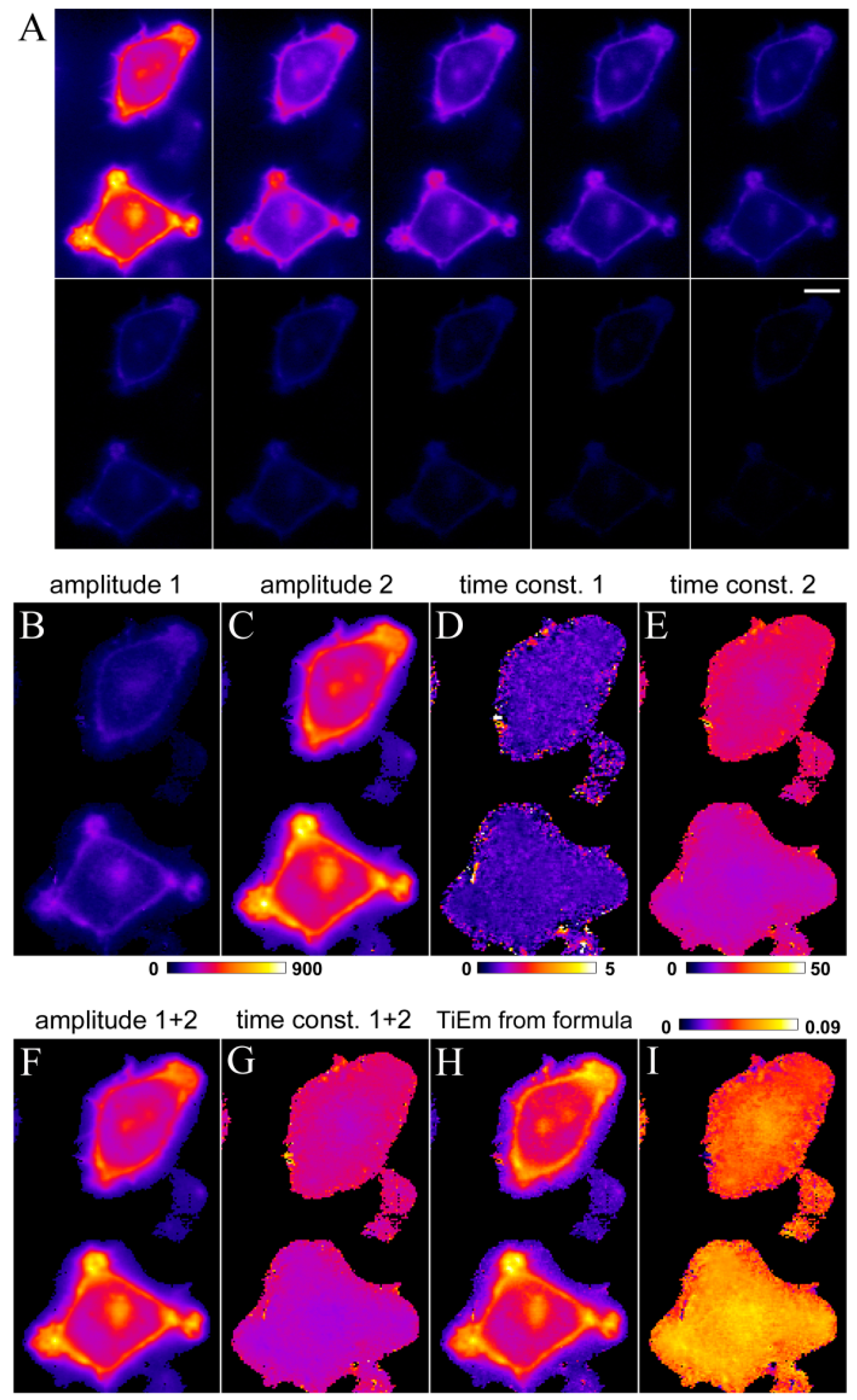
  . Variation in either the intersystem crossing rate constant or the relaxation rate constant from the triplet to the singlet ground state can therefore have profound impacts on the overall bleaching kinetics, especially if the bleach rate constant from the triplet state is significantly higher than that from the excited singlet state (i.e., if k4 >> k2). Both intrinsic bleach rate constants, as well as the triplet yield will vary in different regions of the cell. Also, the TiEm with triplet bleaching is, as shown for the singlet state, conveniently given as product of amplitude- and time-constant-map from a mono-exponential fit to experimental data.
 , and equilibrium constant of the photocycle between the two singlet states,
  . The triplet yield was varied between zero (no triplet occupation) and fifty (high triplet occupation) on the abscissa. Other parameters were as for Figure 4, i.e., an intrinsic bleach rate constant from the excited singlet state, of k2 = 0.01 s−1 and from the excited triplet state of k4 = 0.1 s−1. Variation of the equilibrium constant of the photocycle between the two singlet states, q, is as indicated in the figure.
, and equilibrium constant of the photocycle between the two singlet states, . The triplet yield was varied between zero (no triplet occupation) and fifty (high triplet occupation) on the abscissa. Other parameters were as for Figure 4, i.e., an intrinsic bleach rate constant from the excited singlet state, of k2 = 0.01 s−1 and from the excited triplet state of k4 = 0.1 s−1. Variation of the equilibrium constant of the photocycle between the two singlet states, q, is as indicated in the figure.
. The triplet yield was varied between zero (no triplet occupation) and fifty (high triplet occupation) on the abscissa. Other parameters were as for Figure 4, i.e., an intrinsic bleach rate constant from the excited singlet state, of k2 = 0.01 s−1 and from the excited triplet state of k4 = 0.1 s−1. Variation of the equilibrium constant of the photocycle between the two singlet states, q, is as indicated in the figure.
, and equilibrium constant of the photocycle between the two singlet states, . The triplet yield was varied between zero (no triplet occupation) and fifty (high triplet occupation) on the abscissa. Other parameters were as for Figure 4, i.e., an intrinsic bleach rate constant from the excited singlet state, of k2 = 0.01 s−1 and from the excited triplet state of k4 = 0.1 s−1. Variation of the equilibrium constant of the photocycle between the two singlet states, q, is as indicated in the figure.
2.6. Multi-Exponential Photobleaching of Fluorescent Probes in Living Cells

 and
and  , given by Equations (16) and (37), respectively. It is also possible, that a fluorophore has several distinct lifetimes in different cellular microenvironments. For example, NBD-tagged PC and SM species as well as BChol have been shown to possess bi-exponential fluorescence lifetime decays in living cells [26,56]. Apart from the possibility of more complex photophysics leading to multi-exponential photobleaching as discussed in Section 4, this could be a consequence of different protonation states in the excited state or due to two dye populations with varying quenching sensitivity [63]. Assuming photobleaching from singlet and triplet state (Equation (35)) but now with two different fluorescence lifetimes, this will lead to Equation (39):


 [36].
[36]. 


2.7. Extension of the Photobleaching Model to a Random Distribution of Rate Constants


 , and a power law of time, in which the parameter b plays the same role as the stretching parameter, h, in the classical StrExp function (see Equations (45) and (46), above). We want to stress the point that time-dependent rate coefficients occur naturally in diffusion-limited bimolecular reactions, for example in fast fluorescence quenching [77]. The classical modelling approach for such processes is the Smoluchowski equation, in which the fluorescence decay becomes the sum of an exponential and a StrExp function, in which the stretching parameter is b = 0.5 [78]. Thus, we can further justify our approach by stating that diffusion of oxygen into the LD’s limits the overall bleaching rate.
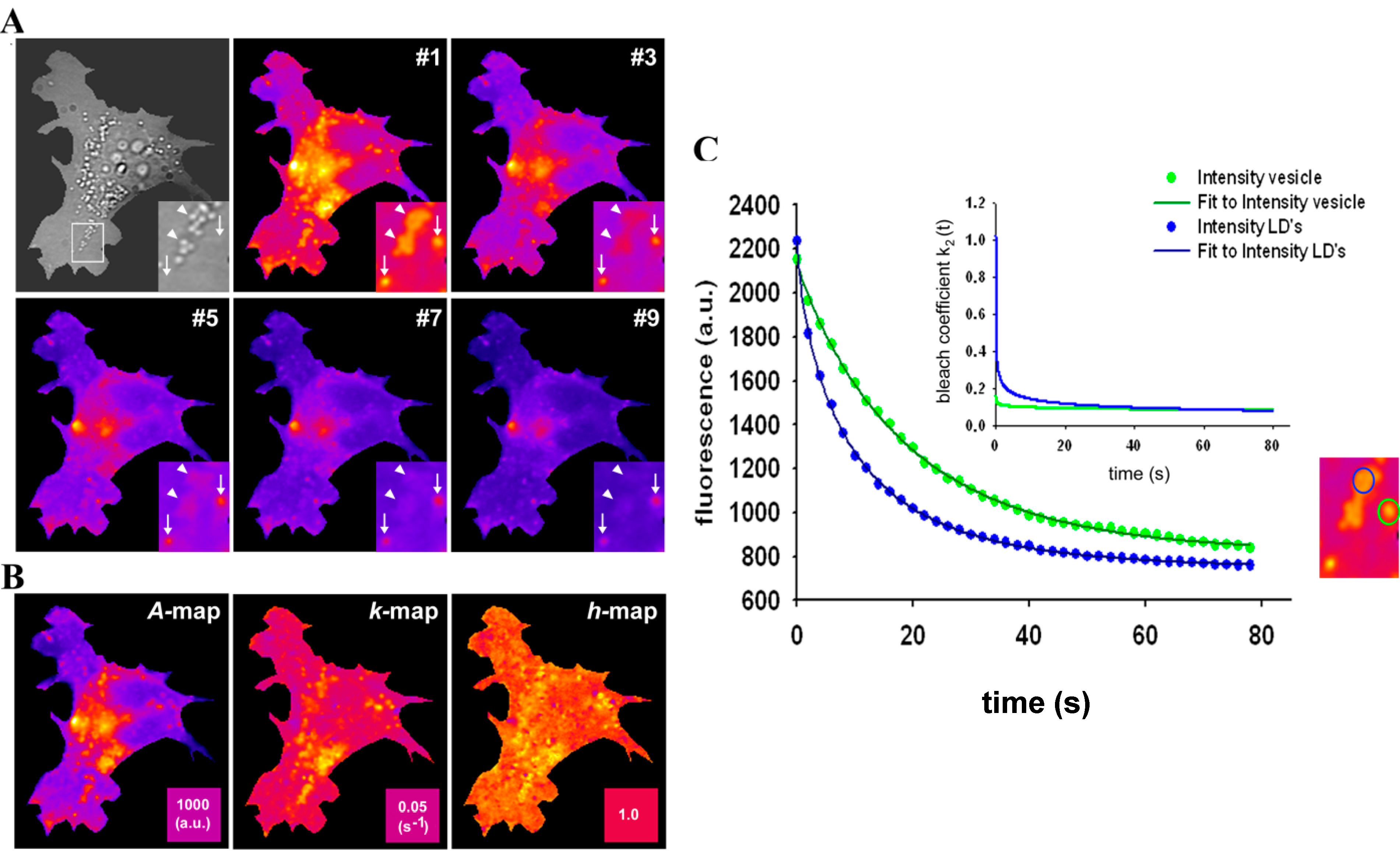
 = 0.2742 s−1 and a much more stretched photobleaching decay (b = 0.2868 than in endocytic vesicles (
  = 0.1145 s−1 and b = 0.0725; see legend to Figure 7 for other parameters). The bleaching rate coefficient, k2(t) slows down over time for both measured areas, but much more pronounced for LD’s. An interpretation could be that LD’s contain large amounts of (singlet) oxygen causing initially fast photo-oxidation of BChol, while over time oxygen gets depleted in LD’s. Assuming that replenishment from other cellular areas is slow compared to the bleach rate, oxygen availability would become rate limiting and thereby slow the photobleaching especially in LD’s. When incubating BHK cells overnight with DHE in complex with albumin, we found targeting of that sterol to LD’s as well, probably as a consequence of DHE esterification. Transport of DHE to LD’s after long time paralleled by its esterification has been found also in other cell types [79]. Interestingly, photobleaching kinetics of DHE were faster in LD’s than in other regions of BHK cells, and followed only in LD’s a stretched exponential decay (not shown). This further supports that LD’s provide a very special environment for photodestruction processes of hydrophobic fluorescent probes.
2.8. TiEm of the Non-Exponential Photobleaching Model


 is the Euler gamma function.
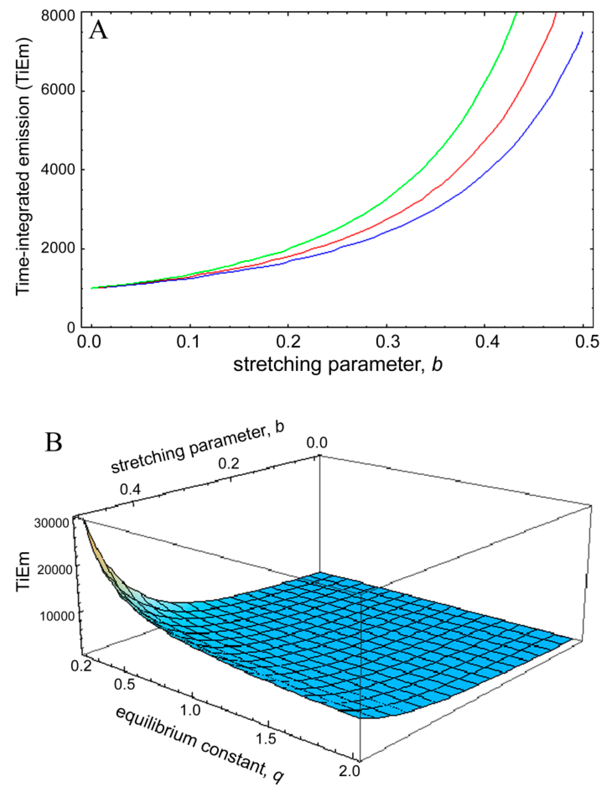
  , was plotted as function of the stretching parameter, b, for M = 100, k2 = 0.1 s−1 and various q-values (Figure 8). The curves in Figure 6A start at = 1,000 for b = 0 and thereby coincide with the TiEm of fluorescence with bleaching from the excited singlet state, , of Equation (16), above. For increasing values of b, we observe an increasing deviation of from with ( − ) > 0, meaning that the TiEm is always larger in case of a rate coefficient than for constant intrinsic bleach rate constant (compare Equations (16) and (50)). Moreover, the difference is larger for small equilibrium constants between S0 and S1 than for large ones (e.g., compare q = 0.5 and q = 2.0; green and blue curve in Figure 8A or 3D plot in Figure 8B). = 1,000. This equals the vsalue of = 1,000 for b = 0. The TiEm for the model, , is plotted for three values of the equilibrium constant of the photocycle, q = 2 (blue curve), q = 1 (red curve) and q = 0.5 photons/molecule (green curve), respectively; (B) 3D plot of the same model with identical parameters but as function of both, b and q. See text for further explanations.
= 1,000. This equals the vsalue of = 1,000 for b = 0. The TiEm for the model, , is plotted for three values of the equilibrium constant of the photocycle, q = 2 (blue curve), q = 1 (red curve) and q = 0.5 photons/molecule (green curve), respectively; (B) 3D plot of the same model with identical parameters but as function of both, b and q. See text for further explanations.
, was plotted as function of the stretching parameter, b, for M = 100, k2 = 0.1 s−1 and various q-values (Figure 8). The curves in Figure 6A start at = 1,000 for b = 0 and thereby coincide with the TiEm of fluorescence with bleaching from the excited singlet state, , of Equation (16), above. For increasing values of b, we observe an increasing deviation of from with ( − ) > 0, meaning that the TiEm is always larger in case of a rate coefficient than for constant intrinsic bleach rate constant (compare Equations (16) and (50)). Moreover, the difference is larger for small equilibrium constants between S0 and S1 than for large ones (e.g., compare q = 0.5 and q = 2.0; green and blue curve in Figure 8A or 3D plot in Figure 8B). = 1,000. This equals the vsalue of = 1,000 for b = 0. The TiEm for the model, , is plotted for three values of the equilibrium constant of the photocycle, q = 2 (blue curve), q = 1 (red curve) and q = 0.5 photons/molecule (green curve), respectively; (B) 3D plot of the same model with identical parameters but as function of both, b and q. See text for further explanations.
= 1,000. This equals the vsalue of = 1,000 for b = 0. The TiEm for the model, , is plotted for three values of the equilibrium constant of the photocycle, q = 2 (blue curve), q = 1 (red curve) and q = 0.5 photons/molecule (green curve), respectively; (B) 3D plot of the same model with identical parameters but as function of both, b and q. See text for further explanations. and for a given value of the stretching parameter, b. Thus, in case of strong illumination, which will saturate the fluorophore, larger deviation of the bleaching kinetics from a mono-exponential decay can be tolerated to keep a meaningful interpretation of the TiEm (see Figure 8A,B). Together, bleaching models with underlying distributions of rate constants might be a suitable alternative to mono-and multi-exponential decay models. In some cases, a mechanistic underpinning for time-dependent rate coefficients is possible, while in other cases they purely serve the purpose of improving the fitting performance. For small deviations from the classical mono-exponential decay (i.e., for narrow distribution of rate constants), the TiEm given by such models can be interpreted as shown for the mono-exponential decay model developed in this study.
 3. Experimental Section
3.1. Reagents and Cell Labelling
3.2. Fluorescence Microscopy, Image Analysis and Simulation
4. Conclusions
Supplementary Materials
Supplementary Files
Supplementary File 1Acknowledgments
Author Contributions
Conflicts of Interest
References
- Sönnichsen, B.; de Renzis, S.; Nielsen, E.; Rietdorf, J.; Zerial, M. Distinct membrane domains on endosomes in the recycling pathway visualized by multicolor imaging of Rab4, Rab5, and Rab11. J. Cell Biol. 2000, 149, 901–914. [Google Scholar] [CrossRef] [PubMed]
- Grant, B.; Hirsh, D. Receptor-mediated endocytosis in the Caenorhabditis elegans oocyte. Mol. Biol. Cell 1999, 10, 4311–4326. [Google Scholar] [CrossRef] [PubMed]
- Ghosh, R.N.; Mallet, W.G.; Soe, T.T.; McGraw, T.E.; Maxfield, F.R. An endocytosed TGN38 chimeric protein is delivered to the TGN after trafficking through the endocytic recycling compartment in CHO cells. J. Cell Biol. 1998, 142, 923–936. [Google Scholar] [CrossRef] [PubMed]
- Chen, I.; Ting, A.Y. Site-specific labeling of proteins with small molecules in live cells. Curr. Opin. Biotechnol. 2005, 16, 35–40. [Google Scholar] [CrossRef] [PubMed]
- Ghosh, R.N.; Gelman, D.L.; Maxfield, F.R. Quantification of low density lipoprotein and transferrin endocytic sorting in HEp2 cells using confocal microscopy. J. Cell Sci. 1994, 107, 2177–2189. [Google Scholar] [PubMed]
- Lipsky, N.G.; Pagano, R.E. A vital stain for the Golgi apparatus. Science 1989, 228, 745–747. [Google Scholar] [CrossRef]
- Pagano, R.E.; Sepanski, M.A.; Martin, O.C. Molecular trapping of a fluorescent ceramide analogue at the Golgi apparatus of fixed cells: Interaction with endogenous lipids provides a trans-Golgi marker for both light and electron microscopy. J. Cell Biol. 1989, 109, 2067–2079. [Google Scholar] [CrossRef] [PubMed]
- Hao, M.; Lin, S.X.; Karylowski, O.J.; Wüstner, D.; McGraw, T.E.; Maxfield, F.R. Vesicular and non-vesicular sterol transport in living cells. The endocytic recycling compartment is a major sterol storage organelle. J. Biol. Chem. 2002, 277, 609–617. [Google Scholar]
- Wüstner, D.; Mondal, M.; Tabas, I.; Maxfield, F.R. Direct observation of rapid internalization and intracellular transport of sterol by macrophage foam cells. Traffic 2005, 6, 396–412. [Google Scholar] [CrossRef] [PubMed]
- Wüstner, D.; Herrmann, A.; Hao, M.; Maxfield, F.R. Rapid nonvesicular transport of sterol between the plasma membrane domains of polarized hepatic cells. J. Biol. Chem. 2002, 277, 30325–30336. [Google Scholar] [CrossRef] [PubMed]
- Mayor, S.; Presley, J.F.; Maxfield, F.R. Sorting of membrane components from endosomes and subsequent recycling to the cell surface occurs by a bulk flow process. J. Cell Biol. 1993, 121, 1257–1269. [Google Scholar] [CrossRef] [PubMed]
- Presley, J.F.; Mayor, S.; McGraw, T.E.; Dunn, K.W.; Maxfield, F.R. Bafilomycin A1 treatment retards transferrin receptor recycling more than bulk membrane recycling. J. Biol. Chem. 1997, 272, 13929–13936. [Google Scholar] [CrossRef] [PubMed]
- Hao, M.; Maxfield, F.R. Characterization of rapid membrane internalization and recycling. J. Biol. Chem. 2000, 275, 15279–15286. [Google Scholar] [CrossRef] [PubMed]
- Van der Sijs, D.A.; van Faassen, E.E.; Levine, Y.K. The interpretation of fluorescence anisotropy decays of probe molecules in membrane systems. Chem. Phys. Lett. 1993, 216, 559–565. [Google Scholar] [CrossRef]
- Illinger, D.; Kuhry, J.-G. The kinetic aspects of intracellular fluorescence labeling with TMA-DPH support the maturation model for endocytosis in L929 cells. J. Cell Biol. 1994, 125, 783–794. [Google Scholar] [CrossRef] [PubMed]
- Florine-Casteel, K. Phospholipid order in gel- and fluid phase cell-size liposomes measured by digitized video fluorescence polarization microscopy. Biophys. J. 1990, 57, 1199–1215. [Google Scholar] [CrossRef] [PubMed]
- Florine-Casteel, K.; Lemasters, J.J.; Herman, B. Lipid order in hepatocyte plasma membrane blebs during ATP-depletion measured by digitized video fluorescence polarization microscopy. FASEB J. 1991, 5, 2078–2084. [Google Scholar] [PubMed]
- Gasecka, A.; Han, T.J.; Favard, C.; Cho, B.R.; Brasselet, S. Quantitative imaging of molecular order in lipid membranes using two-photon fluorescence polarimetry. Biophys. J. 2009, 97, 2854–2862. [Google Scholar] [CrossRef] [PubMed]
- Mukherjee, S.; Soe, T.T.; Maxfield, F.R. Endocytic sorting of lipid analogues differing solely in the chemistry of their hydrophobic tails. J. Cell Biol. 1999, 144, 1271–1284. [Google Scholar] [CrossRef] [PubMed]
- Van Genderen, I.; van Meer, G. Differential targeting of glucosylceramide and galactosylceramide analogues after synthesis but not during transcytosis in Madin-Darby canine kidney cells. J. Cell Biol. 1995, 131, 645–6554. [Google Scholar] [CrossRef] [PubMed]
- Van IJzendoorn, S.C.; Zegers, M.M.; Kok, J.W.; Hoekstra, D. Segregation of glucosylceramide and sphingomyelin occurs in the apical to basolateral transcytotic route in HepG2 cells. J. Cell Biol. 1997, 137, 347–357. [Google Scholar] [CrossRef] [PubMed]
- Wüstner, D.; Mukherjee, S.; Maxfield, F.R.; Müller, P.; Hermann, A. Vesicular and nonvesicular transport of phosphatidylcholine in polarized HepG2 cells. Traffic 2001, 2, 277–296. [Google Scholar] [CrossRef] [PubMed]
- Wüstner, D. Fluorescent sterols as tools in membrane biophysics and cell biology. Chem. Phys. Lipids 2007, 146, 1–25. [Google Scholar] [CrossRef] [PubMed]
- Maxfield, F.R.; Wüstner, D. Analysis of cholesterol trafficking with fluorescent probes. Methods Cell Biol. 2012, 108, 367–393. [Google Scholar] [PubMed]
- Hölttä-Vuori, M.; Uronen, R.L.; Repakova, J.; Salonen, E.; Vattulainen, I.; Panula, P.; Li, Z.; Bittman, R.; Ikonen, E. BODIPY-cholesterol: A new tool to visualize sterol trafficking in living cells and organisms. Traffic 2008, 9, 1839–1849. [Google Scholar] [CrossRef] [PubMed]
- Wüstner, D.; Solanko, L.M.; Sokol, E.; Lund, F.W.; Garvik, O.; Li, Z.; Bittman, R.; Korte, T.; Herrmann, A. Quantitative assessment of sterol traffic in living cells by dual labeling with dehydroergosterol and BODIPY-cholesterol. Chem. Phys. Lipids 2011, 164, 221–235. [Google Scholar] [CrossRef] [PubMed]
- Wüstner, D. Following intracellular cholesterol transport by linear and non-linear optical microscopy of intrinsically fluorescent sterols. Curr. Pharm. Biotechnol. 2012, 13, 303–318. [Google Scholar] [CrossRef] [PubMed]
- Gimpl, G. Cholesterol-protein interaction: Methods and cholesterol reporter molecules. Subcell. Biochem. 2010, 51, 1–45. [Google Scholar] [PubMed]
- Solanko, L.M.; Honigmann, A.; Midtiby, H.S.; Lund, F.W.; Brewer, J.R.; Dekaris, V.; Bittman, R.; Eggeling, C.; Wüstner, D. Membrane orientation and lateral diffusion of BODIPY-cholesterol as a function of probe structure. Biophys. J. 2013, 105, 2082–2092. [Google Scholar] [CrossRef] [PubMed]
- Hiramoto-Yamaki, N.; Tanaka, K.A.; Suzuki, K.G.; Hirosawa, K.M.; Miyahara, M.S.; Kalay, Z.; Tanaka, K.; Kasai, R.S.; Kusumi, A.; Fujiwara, T.K. Ultrafast diffusion of a fluorescent cholesterol analog in compartmentalized plasma membranes. Traffic 2014, 15, 583–612. [Google Scholar] [CrossRef] [PubMed]
- Mazères, S.; Schram, V.; Tocanne, J.F.; Lopez, A. 7-nitrobenz-2-oxa-1,3-diazole-4-yl-labeled phospholipids in lipid membranes: Differences in fluorescence behavior. Biophys. J. 1996, 71, 327–335. [Google Scholar] [CrossRef] [PubMed]
- Benson, D.M.; Bryan, J.; Plant, A.L.; Gotto, A.M.J.; Smith, L.C. Digital imaging fluorescence microscopy: Spatial heterogeneity of photobleaching rate constants in individual cells. J. Cell Biol. 1985, 100, 1309–1323. [Google Scholar] [CrossRef] [PubMed]
- Pagano, R.E.; Longmuir, K.J.; Martin, O.C. Intracellular translocation and metabolism of a fluorescent phosphatidic acid in cultured fibroblasts. J. Biol. Chem. 1983, 258, 2034–2040. [Google Scholar] [PubMed]
- Martin, O.C.; Comly, M.E.; Blanchette-Mackie, E.J.; Pentchev, P.G.; Pagano, R.E. Cholesterol deprivation affects the fluorescence properties of a ceramide analog at the Golgi apparatus of living cells. Proc. Natl. Acad. Sci. USA 1993, 90, 2661–2665. [Google Scholar] [CrossRef] [PubMed]
- Hirschfeld, T. Quantum efficiency independence of the time integrated emission from a fluorescent molecule. Appl. Opt. 1976, 15, 3135–3139. [Google Scholar] [CrossRef] [PubMed]
- Wüstner, D.; Landt Larsen, A.; Færgeman, N.J.; Brewer, J.R.; Sage, D. Selective visualization of fluorescent sterols in Caenorhabditis elegans by bleach-rate based image segmentation. Traffic 2010, 11, 440–454. [Google Scholar] [CrossRef] [PubMed]
- ImageJ RSB Home Page-Image Processing and Analysis in Java. Available online: http://imagej.nih.gov/ij/ (accessed on 1 January 2014).
- Bright, G.R.; Fisher, G.W.; Rogowska, J.; Taylor, D.L. Fluorescence ratio imaging microscopy. Methods Cell Biol. 1989, 30, 157–192. [Google Scholar] [PubMed]
- Jovin, T.M.; Arndt-Jovin, D.J. FRET Microscopy: Digital imaging of fluorescence resonance energy transfer. Applications in cell biology. In Cell Structure and Function by Microspectrofluorometry; Kohen, E., Hirschberg, J.G., Eds.; Academic Press: Waltham, MA, USA, 1989; pp. 99–117. [Google Scholar]
- White, J.C.; Stryer, L. Photostability studies of phycobiliprotein fluorescent labels. Anal. Biochem. 1987, 161, 442–452. [Google Scholar] [CrossRef] [PubMed]
- Ariola, F.S.; Li, Z.; Cornejo, C.; Bittman, R.; Heikal, A.A. Membrane fluidity and lipid order in ternary giant unilamellar vesicles using a new bodipy-cholesterol derivative. Biophys. J. 2009, 96, 2696–2708. [Google Scholar] [CrossRef] [PubMed]
- Chattopadhyay, A. Chemistry and biology of N-(7-nitrobenz-2-oxa-1,3-diazol-4-yl)-labeled lipids: Fluorescent probes of biological and model membranes. Chem. Phys. Lipids 1990, 53, 1–15. [Google Scholar] [CrossRef] [PubMed]
- Marks, D.L.; Bittman, R.; Pagano, R.E. Use of Bodipy-labeled sphingolipid and cholesterol analogs to examine membrane microdomains in cells. Histochem. Cell Biol. 2008, 130, 819–832. [Google Scholar] [CrossRef] [PubMed]
- MacDonald, R.I. Characteristics of self-quenching of the fluorescence of lipid-conjugated rhodamine in membranes. J. Biol. Chem. 1990, 265, 13533–13539. [Google Scholar] [PubMed]
- Ghauharali, R.I.; Müller, M.; Buist, A.H.; Sosnowski, T.S.; Norris, T.B.; Squier, J.; Brakenhoff, G.J. Optical saturation measurements of fluorophores in solution with pulsed femtosecond excitation and two-dimensional CCD camera detection. Appl. Opt. 1997, 36, 4320–4328. [Google Scholar] [CrossRef] [PubMed]
- Lund, F.W.; Wüstner, D. A comparison of single particle tracking and temporal image correlation spectroscopy for quantitative analysis of endosome motility. J. Microsc. 2013, 252, 169–188. [Google Scholar] [CrossRef] [PubMed]
- Dulin, D.; le Gali, A.; Perronet, K.; Soler, N.; Fourmy, D.; Yoshizawa, S.; Bouyer, P.; Westbrook, N. Reduced photobleaching of BODIPY-FL. Phys. Procedia 2010, 3, 1563–1567. [Google Scholar] [CrossRef]
- Deschenes, L.A.; Vanden Bout, D.A. Single molecule photobleaching: Increased photon yield and survival time through suppression of two-step photolysis. Chem. Phys. Lett. 2002, 365, 387–395. [Google Scholar] [CrossRef]
- Kubitscheck, U.; Kircheis, M.; Schweitzer-Stenner, R.; Dreybrodt, W.; Jovin, T.M.; Pecht, I. Fluorescence resonance energy transfer on single living cells. Biophys. J. 1991, 60, 307–318. [Google Scholar] [CrossRef] [PubMed]
- Young, R.M.; Arnette, K.; Roess, D.A.; Barisas, B.G. Quantitation of fluorescence energy transfer between cell surface proteins via fluorescence donor photobleaching kinetics. Biophys. J. 1994, 67, 881–888. [Google Scholar] [CrossRef] [PubMed]
- Szabo, G.; Pine, P.S.; Weaver, J.L.; Kasari, M.; Aszalos, A. Epitope mapping by photobleaching fluorescence resonance energy-transfer measurements using a laser scanning microscope system. Biophys. J. 1992, 61, 661–670. [Google Scholar] [CrossRef] [PubMed]
- Wüstner, D.; Brewer, J.R.; Bagatolli, L.A.; Sage, D. Potential of ultraviolet widefield imaging and multiphoton microscopy for analysis of dehydroergosterol in cellular membranes. Microsc. Res. Tech. 2011, 74, 92–108. [Google Scholar] [CrossRef] [PubMed]
- i>Brandt, S. Datenanalyse; Spektrum Verlag: Heidelberg, Berlin, Germany, 1999. [Google Scholar]
- Wüstner, D.; Solanko, L.M.; Lund, F.W.; Sage, D.; Schroll, J.A.; Lomholt, M.A. Quantitative fluorescence loss in photobleaching for analysis of protein transport and aggregation. BMC Bioinform. 2012, 13, 296. [Google Scholar] [CrossRef] [Green Version]
- Pourmousa, M.; Róg, T.; Mikkeli, R.; Vattulainen, I.; Solanko, L.; Wüstner, D.; List, N.; Kongsted, J.; Karttunen, M. Dehydroergosterol as an analogue for cholesterol: Why it mimics cholesterol so well or does It? J. Phys. Chem. B 2014, 118, 7345–7357. [Google Scholar] [CrossRef]
- Stöckl, M.; Plazzo, A.P.; Korte, T.; Herrmann, A. Detection of lipid domains in model and cell membranes by fluorescence lifetime imaging microscopy of fluorescent lipid analogues. J. Biol. Chem. 2008, 283, 30828–30837. [Google Scholar] [CrossRef] [PubMed]
- Smutzer, G.; Crawford, B.F.; Yeagle, P.L. Physical properties of the fluorescent sterol probe dehydroergosterol. Biochim. Biophys. Acta 1986, 862, 361–371. [Google Scholar] [CrossRef] [PubMed]
- Garvik, O.; Benediktson, P.; Simonsen, A.C.; Ipsen, J.H.; Wüstner, D. The fluorescent cholesterol analog dehydroergosterol induces liquid-ordered domains in model membranes. Chem. Phys. Lipids 2009, 159, 114–118. [Google Scholar] [CrossRef] [PubMed]
- Widengren, J.; Mets, Ü.; Rigler, R. Fluorescence correlation spectroscopy of triplet states in solution: A theoretical and experimental study. J. Phys. Chem. 1995, 99, 13368–13379. [Google Scholar]
- Song, L.; Varma, C.A.; Verhoeven, J.W.; Tanke, H.J. Influence of the triplet excited state on the photobleaching kinetics of fluorescein in microscopy. Biophys. J. 1996, 70, 252959–252968. [Google Scholar] [CrossRef]
- Song, L.; Hennink, E.J.; Young, I.T.; Tanke, H.J. Photobleaching kinetics of fluorescein in quantitative fluorescence microscopy. Biophys. J. 1995, 68, 2588–2600. [Google Scholar] [CrossRef] [PubMed]
- Song, L.; van Gijlswijk, R.P.M.; Young, I.T.; Tanke, H.J. Influence of fluorochrome labeling density on the photobleaching kinetics of fluorescein in microscopy. Cytometry 1997, 27, 213–223. [Google Scholar] [CrossRef] [PubMed]
- Boens, N.; Ameloot, M. Compartmental modeling and identifiability analysis in photophysics: Review. Int. J. Quant. Chem. 2005, 106, 300–315. [Google Scholar] [CrossRef]
- Toptygin, D.; Brand, L. Fluorescence decay of DPH in lipid membranes: Influence of the external refractive index. Biophys. Chem. 1993, 48, 205–220. [Google Scholar] [CrossRef] [PubMed]
- Krishna, M.M.G.; Periasamy, N. Orientational distribution of linear dye molecules in bilayer membranes. Chem. Phys. Lett. 1998, 298, 359–367. [Google Scholar] [CrossRef]
- Listenberger, L.L.; Brown, D.A. Fluorescent detection of lipid droplets and associated proteins. Curr. Protoc. Cell Biol. 2007, 24. [Google Scholar] [CrossRef]
- Berberan-Santos, M.N.; Bodunov, E.N.; Valeur, B. Mathematical functions for the analysis of luminescence decays with underlying distributions 1. Kohlrausch decay function (stretched exponential). Chem. Phys. 2005, 315, 171–182. [Google Scholar]
- Kohlrausch, R. Theorie des elektrischen Rückstandes in der Leidner Flasche. Pogg. Ann. Phys. Chem. 1854, 91, 179–213. [Google Scholar] [CrossRef]
- Berberan-Santos, M.N. Luminescence decays with underlying distributions: General properties and analysis with mathematical functions. J. Luminesc. 2007, 126, 263–272. [Google Scholar] [CrossRef]
- Hinkeldey, B.; Schmitt, A.; Jung, G. Comparative photostability studies of BODIPY and fluorescein dyes by using fluorescence correlation spectroscopy. ChemPhysChem 2008, 9, 2019–2027. [Google Scholar] [CrossRef] [PubMed]
- Berberan-Santos, M.N. Mathematical basis of the integral formalism of chemical kinetics. Compact representation of the general solution of the first-order linear differential equation. J. Math. Chem. 2010, 47, 1184–1188. [Google Scholar]
- Greenbaum, L.; Rothmann, Z.; Lavie, R.; Malik, Z. Green fluorescent protein photobleaching: A model for protein damage by endogenous and exogenous singlet oxygen. Biol. Chem. 2000, 381, 1251–1258. [Google Scholar] [CrossRef] [PubMed]
- Georgakoudi, I.; Foster, T.H. Singlet oxygen-versus nonsinglet oxygen-mediated mechanisms of sensitizer photobleaching and their effects on photodynamic dosimetry. Photochem. Photobiol. 1998, 67, 612–625. [Google Scholar] [CrossRef] [PubMed]
- Lee, P.C.; Rodgers, M.A.J. Singlet molecular oxygen in micellar systems. 1. Distribution Equilibria between hydrophobic and hydrophilic compartments. J. Phys. Chem. 1983, 87, 4894–4898. [Google Scholar]
- Subczynski, W.K.; Hyde, J.S.; Kusumi, A. Oxygen permeability of phosphatidylcholine-Cholesterol membranes. Proc. Natl. Acad. Sci. USA 1989, 86, 4474–4478. [Google Scholar] [CrossRef] [PubMed]
- Bäumler, W.; Regensburger, J.; Knak, A.; Felgenträger, A.; Maisch, T. UVA and endogeneous photosensitizers - the detection of singlet oxygen by its luminescence. Photochem. Photobiol. Sci. 2012, 11, 107–117. [Google Scholar] [CrossRef] [PubMed]
- Sikorski, M.; Krystkowiak, E.; Steer, R.P. The kinetics of fast fluorescence quenching processes. J. Photochem. Photobiol. A Chem. 1998, 117, 1–16. [Google Scholar] [CrossRef]
- Weller, A. Eine verallgemeinerte theorie diffusionsbestimmter reaktionen und ihre anwendung auf die fluoreszenzlöschung. Z. Phys. Chem. 1957, 13, 335–352. [Google Scholar] [CrossRef]
- Mondal, M.; Mesmin, B.; Mukherjee, S.; Maxfield, F.R. Sterols are mainly in the cytoplasmic leaflet of the plasma membrane and the endocytic recycling compartment in CHO cells. Mol. Biol. Cell 2009, 20, 581–588. [Google Scholar] [CrossRef] [PubMed]
- Biomedical Imaging Group. PixBleach - Pixelwise analysis of bleach rate in time-lapse images. Available online: http://bigwww.epfl.ch/algorithms/pixbleach/ (accessed on 1 June 2014).
- Ghauharali, R.I.; Hofstraat, J.W.; Brakenhoff, G.J. Fluorescence photobleaching-based shading correction for fluorescence microscopy. J. Microsc. 1998, 192, 99–113. [Google Scholar] [CrossRef]
- Zwier, J.M.; van Rooij, G.J.; Hofstraat, J.W.; Brakenhoff, G.J. Image calibration in fluorescence microscopy. J. Microsc. 2004, 216, 15–24. [Google Scholar] [CrossRef] [PubMed]
- Koppel, D.E.; Carlson, C.; Smilowitz, H. Analysis of heterogeneous fluorescence photobleaching by video kinetics imaging: The method of cumulants. J. Microsc. 1989, 155, 199–206. [Google Scholar] [CrossRef] [PubMed]
- Van Oostveldt, P.; Verhaegen, F.; Messens, K. Heterogeneous photobleaching in confocal microscopy caused by differences in refractive index and excitation mode. Cytometry 1998, 32, 137–146. [Google Scholar] [CrossRef] [PubMed]
- Kalyansundaram, K.; Thomas, J.K. Environmental effects on vibronic band intensities in pyrene monomer fluorescence and their application in studies of micellar systems. J. Am. Chem. Soc. 1977, 99, 2039–2044. [Google Scholar] [CrossRef]
- Somerharju, P. Pyrene-labeled lipids as tools in membrane biophysics and cell biology. Chem. Phys. Lett. 2002, 116, 57–74. [Google Scholar]
- Albro, P.W.; Bilski, P.; Corbett, J.T.; Schroeder, J.L.; Chignell, C.F. Photochemical reactions and phototoxicity of sterols: Novel self-perpetuating mechanisms for lipid photoxidation. Photochem. Photobiol. 1997, 66, 316–325. [Google Scholar] [CrossRef] [PubMed]
- Eggeling, C.; Widengren, J.; Rigler, R.; Seidel, C.A.M. Photobleaching of fluorescent dyes under conditions used for single-molecule detection: Evidence of two-step photolysis. Anal. Chem. 1998, 70, 2651–2659. [Google Scholar] [CrossRef] [PubMed]
- Gensch, T.; Böhmer, M.; Aramendia, P.F. Single molecule blinking and photobleaching separated by wide-field fluorescence microscopy. J. Phys. Chem. 2005, 109, 6652–6658. [Google Scholar] [CrossRef]
- Bernas, T.; Zaresbski, M.; Cook, R.R.; Dobrucki, J.W. Minimizing photobleaching during confocal microscopy of fluorescent probes bound to chromatin: Role of anoxia and photon flux. J. Microscopy 2004, 215, 281–296. [Google Scholar] [CrossRef]
- Baranyai, P.; Gangl, S.; Grabner, G.; Knapp, M.; Köhler, G.; Vidoczy, T. Using the decay of incorporated photoexcited triplet probes to study unilamellar phospholipid bilayer membranes. Langmuir 1999, 15, 7577–7584. [Google Scholar] [CrossRef]
- Murray, J.M.; Appleton, P.L.; Swedlow, J.R.; Waters, J.C. Evaluating performance in three-dimensional fluorescence microscopy. J. Microscopy 2007, 228, 390–405. [Google Scholar] [CrossRef]
- Velez, M.; Axelrod, D. Polarized fluorescence photobleaching recovery for measuring rotational diffusion in solutions and membranes. Biophys. J. 1988, 53, 575–591. [Google Scholar] [CrossRef] [PubMed]
- Sinnecker, D.; Voigt, P.; Hellwig, N.; Schaefer, M. Reversible photobleaching of enhanced green fluorescent proteins. Biochemistry 2005, 44, 7085–7094. [Google Scholar] [CrossRef] [PubMed]
- Mueller, F.; Morisaki, T.; Mazza, D.; McNally, J.G. Minimizing the impact of photoswitching of fluorescent proteins on FRAP analysis. Biophys. J. 2012, 102, 1656–1665. [Google Scholar] [CrossRef] [PubMed]
- Daddysman, M.K.; Fecko, C.J. Revisiting point FRAP to quantitatively characterize anomalous diffusion in live cells. J. Phys. Chem. 2013, 117, 1241–1251. [Google Scholar] [CrossRef]
- Ringemann, C.; Schönle, A.; Giske, A.; von Middendorff, C.; Hell, S.W.; Eggeling, C. Enhancing fluorescence brightness: Effect of reverse intersystem crossing studied by fluorescence fluctuation spectroscopy. ChemPhysChem 2008, 9, 612–624. [Google Scholar] [CrossRef] [PubMed]
- Füreder-Kitzmüller, E.; Hesse, J.; Ebner, A.; Gruber, H.J.; Schütz, G.J. Non-exponential bleaching of single bioconjugated Cy5 molecules. Chem. Phys. Lett. 2005, 404, 13–18. [Google Scholar] [CrossRef]
- Levin, P.P.; Costa, S.M.P. Kinetics of oxygen induced delayed fluorescence of eosin adsorbed on alumina. The dependence on dye and oxygen concentrations. Chem. Phys. Lett. 2000, 320, 194–201. [Google Scholar]
- Sample Availability: Not available.
© 2014 by the authors. Licensee MDPI, Basel, Switzerland. This article is an open access article distributed under the terms and conditions of the Creative Commons Attribution license ( http://creativecommons.org/licenses/by/3.0/).
Share and Cite
Wüstner, D.; Christensen, T.; Solanko, L.M.; Sage, D. Photobleaching Kinetics and Time-Integrated Emission of Fluorescent Probes in Cellular Membranes. Molecules 2014, 19, 11096-11130. https://doi.org/10.3390/molecules190811096
Wüstner D, Christensen T, Solanko LM, Sage D. Photobleaching Kinetics and Time-Integrated Emission of Fluorescent Probes in Cellular Membranes. Molecules. 2014; 19(8):11096-11130. https://doi.org/10.3390/molecules190811096
Chicago/Turabian StyleWüstner, Daniel, Tanja Christensen, Lukasz M. Solanko, and Daniel Sage. 2014. "Photobleaching Kinetics and Time-Integrated Emission of Fluorescent Probes in Cellular Membranes" Molecules 19, no. 8: 11096-11130. https://doi.org/10.3390/molecules190811096