The Cartesian Product and Join Graphs on Edge-Version Atom-Bond Connectivity and Geometric Arithmetic Indices

Abstract

The Cartesian product and join are two classical operations in graphs. Let $d_{L(G)}(e)$ be the degree of a vertex $e$ in line graph $L(G)$ of a graph $G$. The edge versions of atom-bond connectivity ($AB{C}_e$) and geometric arithmetic ($G{A}_e$) indices of G are defined as ${\displaystyle \sum _{ef\in E(L(G))}\sqrt{\frac{d_{L(G)}(e)+d_{L(G)}(f)-2}{d_{L(G)}(e)\times d_{L(G)}(f)}}}$ and ${\displaystyle \sum _{ef\in E(L(G))}\frac{2\sqrt{d_{L(G)}(e)\times d_{L(G)}(f)}}{d_{L(G)}(e)+d_{L(G)}(f)}}$, respectively. In this paper, $AB{C}_e$ and $G{A}_e$ indices for certain Cartesian product graphs (such as $P_n\square P_m$, $P_n\square C_m$ and $P_n\square S_m$) are obtained. In addition, $AB{C}_e$ and $G{A}_e$ indices of certain join graphs (such as $C_m+P_n+S_r$, $P_m+P_n+P_r$, $C_m+C_n+C_r$ and $S_m+S_n+S_r$) are deduced. Our results enrich and revise some known results.

1. Introduction

The invariants based on the distance or degree of vertices in molecules are called topological indices. In theoretical chemistry, physics and graph theory, topological indices are the molecular descriptors that describe the structures of chemical compounds, and they help us to predict certain physico-chemical properties. The first topological index, Wiener index, was published in 1947 [1], and the edge version of the Wiener index was proposed by Iranmanesh et al. in 2009 [2]. Because the important effects of the topological indices are proved in chemical research, more and more topological indices are studied, including the classical atom-bond connectivity index and the geometric arithmetic index.

Let $G$ be a simple connected graph. Denote by $V(G)$ and $E(G)$ the vertex set and edge set of $G$, respectively. Let $P_n$, $C_n$, $K_n$ and $S_n$ be a path, a cycle, a complete graph and a star, respectively, on $n$ vertices. $e=uv$ represents edge-connecting vertices $u$ and $v$. $N(v)$ is an open neighborhood of vertex $v$, i.e., $N(v)=\left\{u\right|uv\in E(G)\}$. Denote by $d_G(v)$ (simply $d(v)$) the degree of vertex $v$ of graph $G$, i.e., $d(v)=|N(v)|$. Let $L(G)$ or $G^L$ be the line graph of $G$ such that each vertex of $L(G)$ represents an edge of $G$ and two vertices of $L(G)$ are adjacent if and only if their corresponding edges share a common endpoint in $G$ [3]. It is known that the line graph $L(G)$ of any graph $G$ is claw-free. Denote by $d_{L(G)}(e)$ the degree of edge $e$ in $G$, which is the number of edges sharing a common endpoint with edge $e$ in $G$, or the degree of vertex $e$ in $L(G)$. We denote by $E_{n,m}$ (or $E_{n,m}^L$) the set of edges $uv$ with degrees $n$ and $m$ of end vertices $u$ and $v$ in $G$ (or in $G^L$), i.e., $E_{n,m}=\left\{uv\right|\{n,m\}=\{d(u),d(v)\},$ $u\in G,v\in G\}$ or $E_{n,m}^L=\left\{uv\right|\{n,m\}=\{d(u),d(v)\},u\in L(G),v\in L(G)\}$. The distance $d_G(u,v)$ (or $d(u,v)$ for short) between $u$ and $v$ in $G$ is the length of a shortest $u-v$ path.

The atom-bond connectivity (ABC) index was proposed by Estrada et al. in 1998 [4]. The ABC index is defined as:

$$ABC(G)={\displaystyle \sum _{uv\in E(G)}\sqrt{\frac{d_G(u)+d_G(v)-2}{d_G(u)\times d_G(v)}}}$$

(1)

where $d_G(u)$ and $d_G(v)$ are the degrees of the vertices $u$ and $v$ in $G$. Meanwhile, the edge version of the ABC index is:

$$AB{C}_e(G)={\displaystyle \sum _{ef\in E(L(G))}\sqrt{\frac{d_{L(G)}(e)+d_{L(G)}(f)-2}{d_{L(G)}(e)\times d_{L(G)}(f)}}}$$

(2)

where $d_{L(G)}(e)$ and $d_{L(G)}(f)$ are the degrees of the edges $e$ and $f$, respectively, in $G$. The recent research on edge version ABC index can be referred to Gao et al. [5].

The geometric arithmetic (GA) index was proposed by Vukicevic and Furthla in 2009 [6]. The GA index is defined as

$$GA(G)={\displaystyle \sum _{uv\in E(G)}\frac{2\sqrt{d_G(u)d_G(v)}}{d_G(u)+d_G(v)}}$$

(3)

The edge version of the GA index was proposed by Mahmiani et al. [7] and is

$$G{A}_e(G)={\displaystyle \sum _{ef\in E(L(G))}\frac{2\sqrt{d_{L(G)}(e)d_{L(G)}(f)}}{d_{L(G)}(e)+d_{L(G)}(f)}}$$

(4)

Recent research on the edge-version GA index can be referred to the articles [5,8,9,10,11,12,13,14,15,16]. In addition, Das [17] obtained the upper and lower bounds of the ABC index of trees. Furtula et al. [18] found the chemical trees with extremal ABC values. Fath-Tabar et al. [19] obtained some inequalities for the ABC index of a series of graph operations. Chen et al. [20] obtained some upper bounds for the ABC index of graphs with given vertex connectivity. Das and Trinajstić [21] compared the GA and ABC indices for chemical trees and molecular graphs. Xing et al. [22] gave the upper bound for the ABC index of trees with perfect matching and characterized the unique extremal tree.

Based on the results, $AB{C}_e$ and $G{A}_e$ indices for certain Cartesian product graphs (such as $P_n\square P_m$, $P_n\square C_m$ and $P_n\square S_m$) are obtained. In addition, $AB{C}_e$ and $G{A}_e$ indices of certain join graphs (such as $C_m+P_n+S_r$, $P_m+P_n+P_r$, $C_m+C_n+C_r$ and $S_m+S_n+S_r$) are deduced. Our results extend and enrich some known results [5,23,24].

2. Main Results

It is known that the Cartesian product and join operation are very complicated. In this section, we present these two classical type of graphs.

2.1. Cartesian Product Graphs

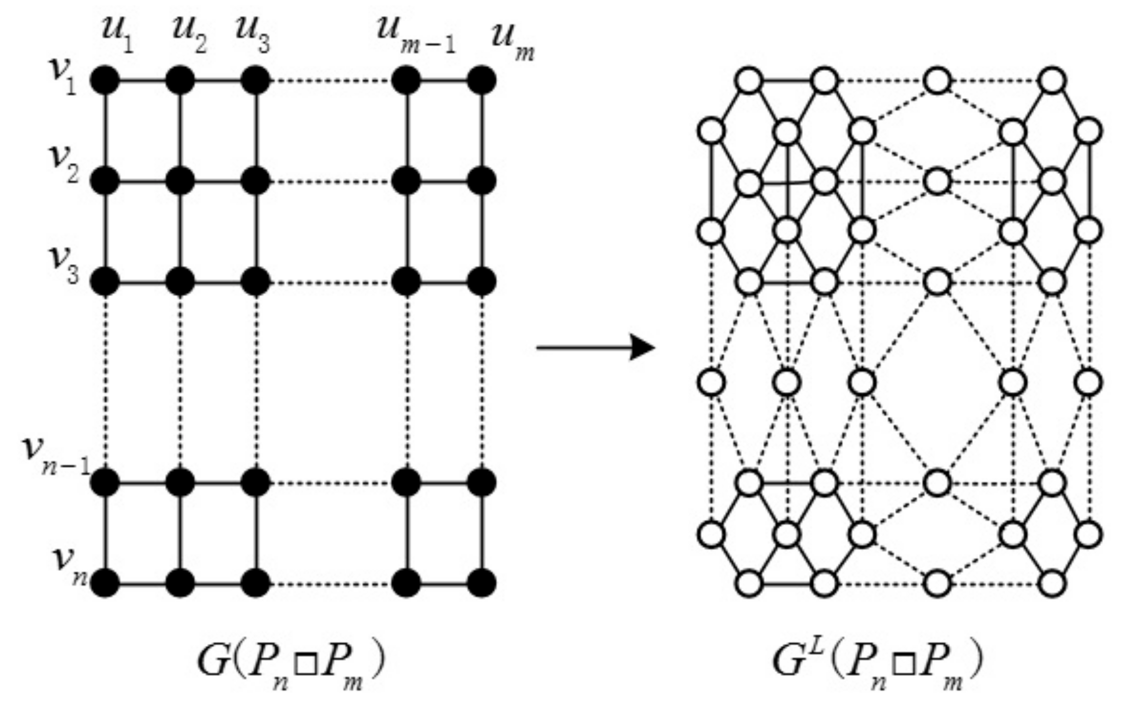
In graph theory, the Cartesian product $G\square H$ of graphs $G$ and $H$ is a graph such that the vertex set of $G\square H$ is the Cartesian product $V(G)\times V(H)$; and any two vertices ($u,u^{\prime }$) and ($v,v^{\prime }$) are adjacent in $G\square H$ if and only if either $u=v$ and $u^{\prime }$ are adjacent with $v^{\prime }$ in $H$ or $u^{\prime }=v^{\prime }$ and $u$ are adjacent with $v$ in $G$. The graph $P_n\square P_m$ and the line graph of $P_n\square P_m$ are illustrated in Figure 1. In the following, we discuss the edge-version ABC and GA indices of some Cartesian product graphs.

Theorem 1. 

If$n,m\ge 4$, then

$$\begin{array}{ll}AB{C}_e(P_n\square P_m)& =\frac{1}{2}\sqrt{\frac{3}{2}}(2n+2m-16)+\frac{1}{2}\sqrt{\frac{7}{5}}(4n+4m-24)+\sqrt{\frac{3}{10}}(6n+6m-32)\\ & +\frac{\sqrt{10}}{6}(6nm-18n-18m+52)+\frac{8\sqrt{2}}{5}+4\sqrt{\frac{5}{3}}+8\sqrt{\frac{2}{5}}+\frac{8}{3};\end{array}$$

(5)

$$\begin{array}{ll}G{A}_e(P_n\square P_m)& =6nm-16n-16m+\frac{4\sqrt{5}}{9}(4n+4m-24)+\frac{2\sqrt{30}}{11}(6n+6m-32)\\ & +44+\frac{16\sqrt{12}}{7}+2\sqrt{15}.\end{array}$$

(6)

Proof. 

Let $G=P_n\square P_m$, we have $L(G)$ has $6nm-6n-6m+4$ edges. Moreover, $\left|E_{3,3}^L\right|=4$, $\left|E_{3,4}^L\right|=8$, $\left|E_{3,5}^L\right|=8$, $\left|E_{4,4}^L\right|=2n+2m-16$, $\left|E_{4,5}^L\right|=4n+4m-24$, $\left|E_{5,5}^L\right|=4$, $\left|E_{5,6}^L\right|=6n+6m-32$ and $\left|E_{6,6}^L\right|=6nm-18n-18m+52$.

$$\begin{array}{ll}AB{C}_e(P_n\square P_m)& =(4)(\sqrt{\frac{3+3-2}{3\times 3}})+(8)(\sqrt{\frac{3+4-2}{3\times 4}})+(8)(\sqrt{\frac{3+5-2}{3\times 5}})\\ & +(2n+2m-16)(\sqrt{\frac{4+4-2}{4\times 4}})\\ & +(4n+4m-24)(\sqrt{\frac{4+5-2}{4\times 5}})+(4)(\sqrt{\frac{5+5-2}{5\times 5}})\\ & +(6n+6m-32)(\sqrt{\frac{5+6-2}{5\times 6}})\\ & +(6nm-18n-18m+52)(\sqrt{\frac{6+6-2}{6\times 6}})\\ & =\frac{1}{2}\sqrt{\frac{3}{2}}(2n+2m-16)+\frac{1}{2}\sqrt{\frac{7}{5}}(4n+4m-24)\\ & +\sqrt{\frac{3}{10}}(6n+6m-32)+\frac{\sqrt{10}}{6}(6nm-18n-18m+52)\\ & +\frac{8\sqrt{2}}{5}+4\sqrt{\frac{5}{3}}+8\sqrt{\frac{2}{5}}+\frac{8}{3};\end{array}$$

(7)

$$\begin{array}{ll}G{A}_e(P_n\square P_m)& =(4)(\frac{2\sqrt{3\times 3}}{3+3})+(8)(\frac{2\sqrt{3\times 4}}{3+4})+(8)(\frac{2\sqrt{3\times 5}}{3+5})\\ & +(2n+2m-16)(\frac{2\sqrt{4\times 4}}{4+4})\\ & +(4n+4m-24)(\frac{2\sqrt{4\times 5}}{4+5})+(4)(\frac{2\sqrt{5\times 5}}{5+5})\\ & +(6n+6m-32)(\frac{2\sqrt{5\times 6}}{5+6})\\ & +(6nm-18n-18m+52)(\frac{2\sqrt{6\times 6}}{6+6})\\ & =6nm-16n-16m+\frac{4\sqrt{5}}{9}(4n+4m-24)\\ & +\frac{2\sqrt{30}}{11}(6n+6m-32)+44+\frac{16\sqrt{12}}{7}+2\sqrt{15}.\end{array}$$

(8)

By now, the proof is complete.

Theorem 2. 

If$n\ge 4,m\ge 3$, then

$$AB{C}_e(P_n\square C_m)=\sqrt{10}nm+(\frac{\sqrt{6}}{2}+2\sqrt{\frac{7}{5}}+\frac{3\sqrt{30}}{5}-\frac{9\sqrt{10}}{3})m$$

(9)

$$G{A}_e(P_n\square C_m)=6nm+(2+\frac{16\sqrt{5}}{9}+\frac{12\sqrt{30}}{11}-18)m$$

(10)

Proof. 

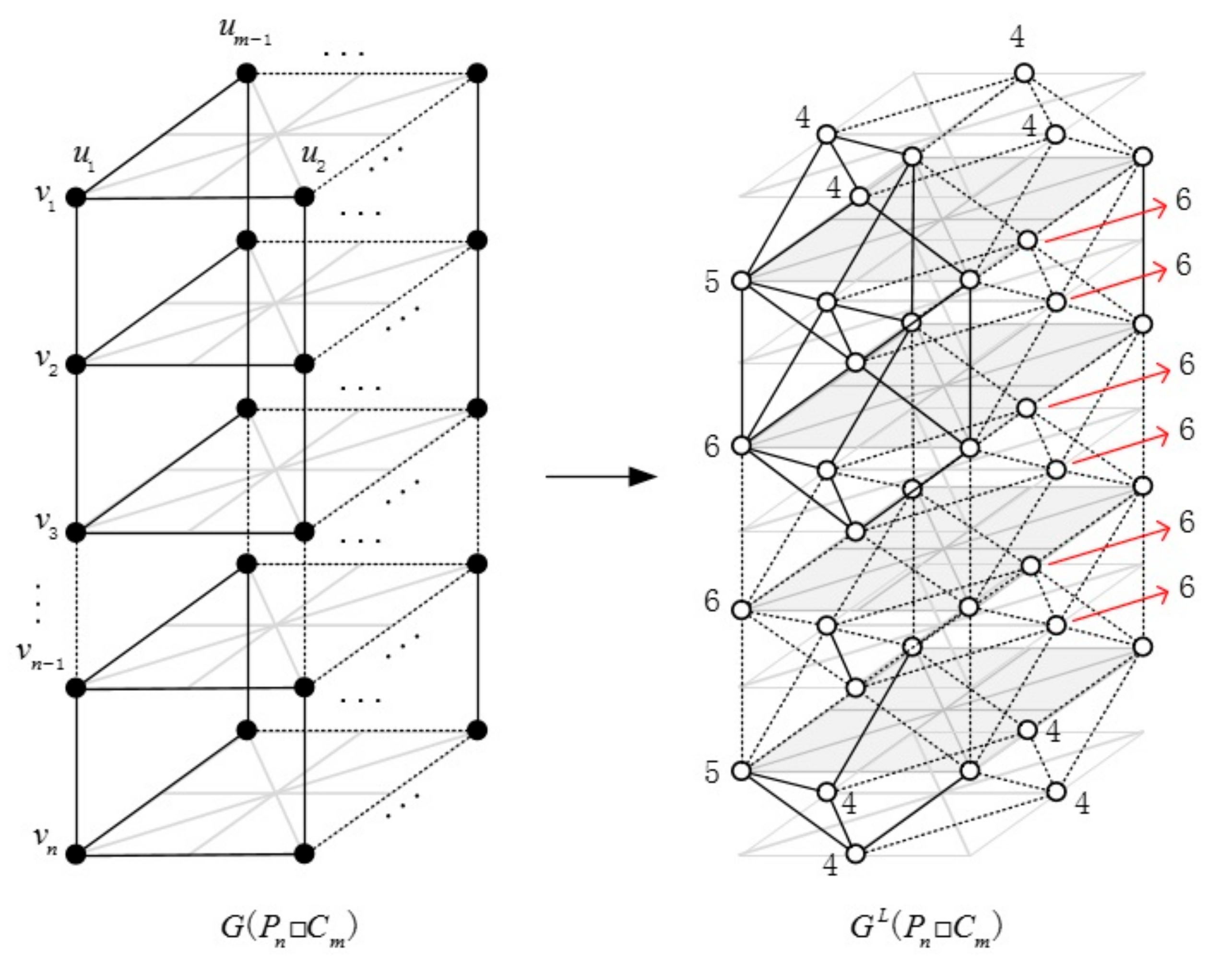
Let $G=P_n\square C_m$, we have $L(G)$ has $6nm-6m$ edges. Moreover, $\left|E_{4,4}^L\right|=2m$, $\left|E_{4,5}^L\right|=4m$, $\left|E_{5,6}^L\right|=6m$ and $\left|E_{6,6}^L\right|=6nm-18m$. In Figure 2, the degrees of vertices in line graph $G^L(P_n\square C_m)$ are displayed near the corresponding vertices.

$$\begin{array}{ll}AB{C}_e(P_n\square C_m)& =(2m)(\sqrt{\frac{4+4-2}{4\times 4}})+(4m)(\sqrt{\frac{4+5-2}{4\times 5}})\\ & +(6m)(\sqrt{\frac{5+6-2}{5\times 6}})+(6nm-18m)(\sqrt{\frac{6+6-2}{6\times 6}})\\ & =\sqrt{10}nm+(\frac{\sqrt{6}}{2}+2\sqrt{\frac{7}{5}}+\frac{3\sqrt{30}}{5}-\frac{9\sqrt{10}}{3})m;\end{array}$$

(11)

$$\begin{array}{ll}G{A}_e(P_n\square C_m)& =(2m)(\frac{2\sqrt{4\times 4}}{4+4})+(4m)(\frac{2\sqrt{4\times 5}}{4+5})+(6m)(\frac{2\sqrt{5\times 6}}{5+6})\\ & +(6nm-18m)(\frac{2\sqrt{6\times 6}}{6+6})\\ & =6nm+(2+\frac{16\sqrt{5}}{9}+\frac{12\sqrt{30}}{11}-18)m.\end{array}$$

(12)

In the end, the proof is complete.

Theorem 3. 

If$n\ge 5,m\ge 1$, then

$$\begin{array}{ll}AB{C}_e(P_n\square S_m)& =\frac{(n-2)(m-1)(m-2)}{2(m+2)}\sqrt{2m+2}\\ & +(n-3)(m-1)(\sqrt{\frac{m+4}{m+2}}+2\sqrt{\frac{3}{2(m+2)}})\\ & +2(m-1)(\sqrt{\frac{m+3}{3(m+2)}}+\sqrt{\frac{3m-1}{(m+2)(2m-1)}}+\sqrt{\frac{m+1}{3m}}\\ & +\sqrt{\frac{3m-3}{m(2m-1)}})+\frac{(m-1)(m-2)}{m}\sqrt{2m-2}\\ & +\frac{1}{4}(m-1)(n-4)\sqrt{6}+(m-1)\sqrt{\frac{5}{3}}\\ & +\frac{n-4}{2m}\sqrt{4m-2}+2\sqrt{\frac{4m-3}{2m(2m-1)}};\end{array}$$

(13)

$$\begin{array}{ll}G{A}_e(P_n\square S_m)& =\frac{(n-2)(m-1)(m-2)}{2}+8(n-3)(m-1)\frac{\sqrt{(m+2)}}{m+6}\\ & +4(m-1)\frac{\sqrt{3(m+2)}}{m+5}+4(n-3)(m-1)\frac{\sqrt{2m(m+2)}}{3m+2}\\ & +4(m-1)\frac{\sqrt{(m+2)(2m-1)}}{3m+1}+(m-1)(m-2)\\ & +4(m-1)\frac{\sqrt{3m}}{m+3}+4(m-1)\frac{\sqrt{m(2m-1)}}{3m-1}\\ & +(m-1)(n-4)+8(m-1)\frac{\sqrt{3}}{7}\\ & +(n-4)+4\frac{\sqrt{2m(2m-1)}}{4m-1}.\end{array}$$

(14)

Proof. 

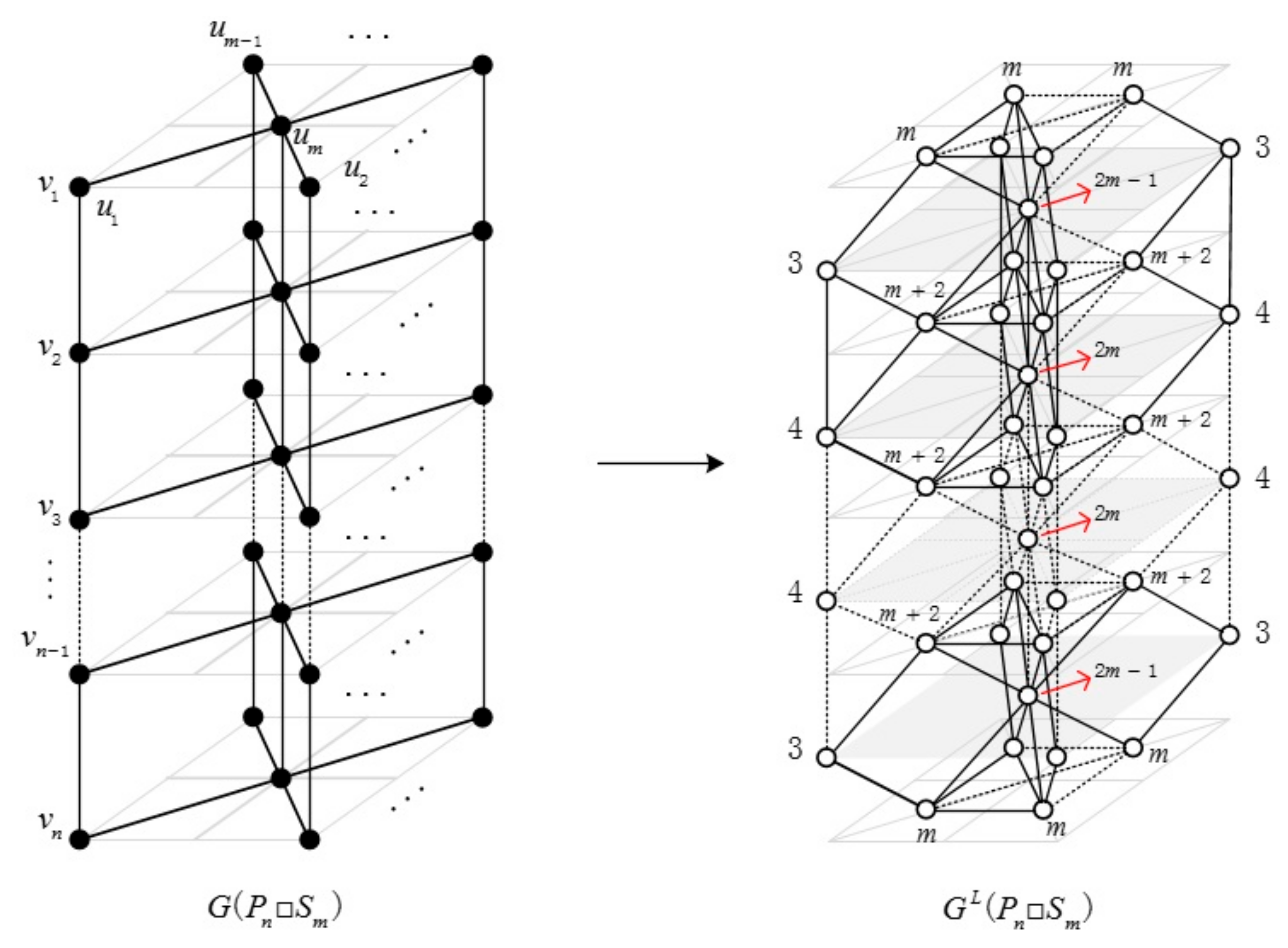
Let $G=P_n\square S_m$, we have $L(G)$ has $\frac{1}{2}(m^{2}n+m(7n-10)-8n+8)$ edges. Moreover, $\left|E_{m+2,m+2}^L\right|=\frac{(n-2)(m-1)(m-2)}{2}$, $\left|E_{m+2,4}^L\right|=2(n-3)(m-1)$, $\left|E_{m+2,3}^L\right|=2(m-1)$, $\left|E_{m+2,2m}^L\right|=2(n-3)(m-1)$, $\left|E_{m+2,2m-1}^L\right|=2(m-1)$, $\left|E_{m,m}^L\right|=(m-1)(m-2)$, $\left|E_{m,3}^L\right|=2(m-1)$, $\left|E_{m,2m-1}^L\right|=2(m-1)$, $\left|E_{4,4}^L\right|=(m-1)(n-4)$, $\left|E_{3,4}^L\right|=2(m-1)$, $\left|E_{2m,2m}^L\right|=(n-4)$ and $\left|E_{2m-1,2m}^L\right|=2$. In Figure 3, the degrees of vertices in line graph $G^L(P_n\square S_m)$ are displayed near by the corresponding vertices.

$$\begin{array}{ll}AB{C}_e(P_n\square S_m)& =\frac{(n-2)(m-1)(m-2)}{2}(\sqrt{\frac{m+2+m+2-2}{(m+2)\times (m+2)}})\\ & +2(n-3)(m-1)(\sqrt{\frac{m+2+4-2}{(m+2)\times 4}})\\ & +2(m-1)(\sqrt{\frac{m+2+3-2}{(m+2)\times 3}})\\ & +2(n-3)(m-1)(\sqrt{\frac{m+2+2m-2}{(m+2)\times 2m}})\\ & +2(m-1)(\sqrt{\frac{m+2+2m-1-2}{(m+2)\times (2m-1)}})\\ & +(m-1)(m-2)(\sqrt{\frac{m+m-2}{m\times m}})\\ & +2(m-1)(\sqrt{\frac{m+3-2}{m\times 3}})+2(m-1)(\sqrt{\frac{m+2m-1-2}{m\times (2m-1)}})\\ & +(m-1)(n-4)(\sqrt{\frac{4+4-2}{4\times 4}})+2(m-1)(\sqrt{\frac{3+4-2}{3\times 4}})\\ & +(n-4)(\sqrt{\frac{2m+2m-2}{2m\times 2m}})+2(\sqrt{\frac{2m-1+2m-2}{(2m-1)\times 2m}})\\ & =\frac{(n-2)(m-1)(m-2)}{2(m+2)}\sqrt{2m+2}\\ & +(n-3)(m-1)(\sqrt{\frac{m+4}{m+2}}+2\sqrt{\frac{3}{2(m+2)}})\\ & +2(m-1)(\sqrt{\frac{m+3}{3(m+2)}}+\sqrt{\frac{3m-1}{(m+2)(2m-1)}}\\ & +\sqrt{\frac{m+1}{3m}}+\sqrt{\frac{3m-3}{m(2m-1)}})\\ & +\frac{(m-1)(m-2)}{m}\sqrt{2m-2}\\ & +\frac{1}{4}(m-1)(n-4)\sqrt{6}+(m-1)\sqrt{\frac{5}{3}}\\ & +\frac{n-4}{2m}\sqrt{4m-2}+2\sqrt{\frac{4m-3}{2m(2m-1)}};\end{array}$$

(15)

$$\begin{array}{ll}G{A}_e(P_n\square S_m)& =\frac{(n-2)(m-1)(m-2)}{2}(\frac{2\sqrt{(m+2)\times (m+2)}}{m+2+m+2})\\ & +2(n-3)(m-1)(\frac{2\sqrt{(m+2)\times 4}}{m+2+4})\\ & +2(m-1)(\frac{2\sqrt{(m+2)\times 3}}{m+2+3})\\ & +2(n-3)(m-1)(\frac{2\sqrt{(m+2)\times 2m}}{m+2+2m})\\ & +2(m-1)(\frac{2\sqrt{(m+2)\times (2m-1)}}{m+2+2m-1})\\ & +(m-1)(m-2)(\frac{2\sqrt{m\times m}}{m+m})\\ & +2(m-1)(\frac{2\sqrt{m\times 3}}{m+3})+2(m-1)(\frac{2\sqrt{m\times (2m-1)}}{m+2m-1})\\ & +(m-1)(n-4)(\frac{2\sqrt{4\times 4}}{4+4})+2(m-1)(\frac{2\sqrt{3\times 4}}{3+4})\\ & +(n-4)(\frac{2\sqrt{2m\times 2m}}{2m+2m})+2(\frac{2\sqrt{(2m-1)\times (2m)}}{2m-1+2m})\\ & =\frac{(n-2)(m-1)(m-2)}{2}+8(n-3)(m-1)\frac{\sqrt{(m+2)}}{m+6}\\ & +4(m-1)\frac{\sqrt{3(m+2)}}{m+5}+4(n-3)(m-1)\frac{\sqrt{2m(m+2)}}{3m+2}\\ & +4(m-1)\frac{\sqrt{(m+2)(2m-1)}}{3m+1}+(m-1)(m-2)\\ & +4(m-1)\frac{\sqrt{3m}}{m+3}+4(m-1)\frac{\sqrt{m(2m-1)}}{3m-1}\\ & +(m-1)(n-4)+8(m-1)\frac{\sqrt{3}}{7}\\ & +(n-4)+4\frac{\sqrt{2m(2m-1)}}{4m-1}.\end{array}$$

(16)

Until now, the proof is complete.

2.2. Join Graph

The results of $AB{C}_e$ and $G{A}_e$ indices of $P_n$, $S_n$, $K_n$ and $C_n$, which were first established by [7], as well as the $AB{C}_e$ and $G{A}_e$ indices of some join graphs, such as $P_n+C_m$, $P_n+S_m$, $C_m+P_n+C_m$, $S_m+P_n+S_m$ and $C_m+P_n+S_r$, created by $P_n$, $C_n$ and $S_n$ were obtained by [5]. However, there are some problems in the calculation of the $AB{C}_e$ and $G{A}_e$ indices of join graph $C_m+P_n+S_r$ in [5].

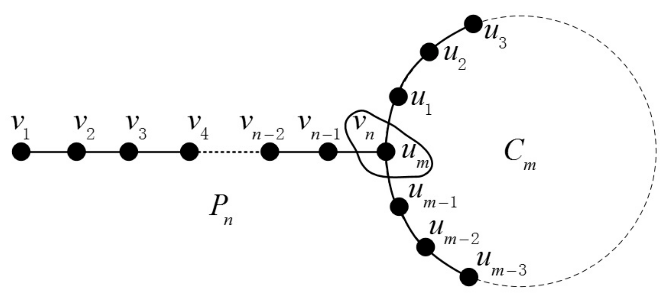
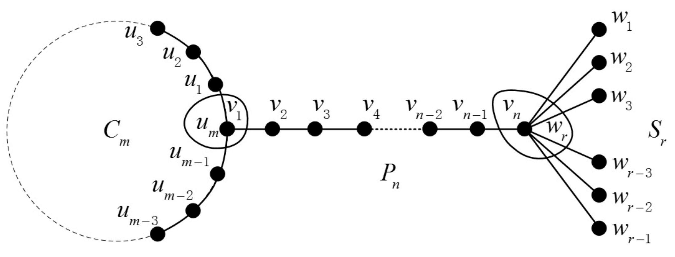
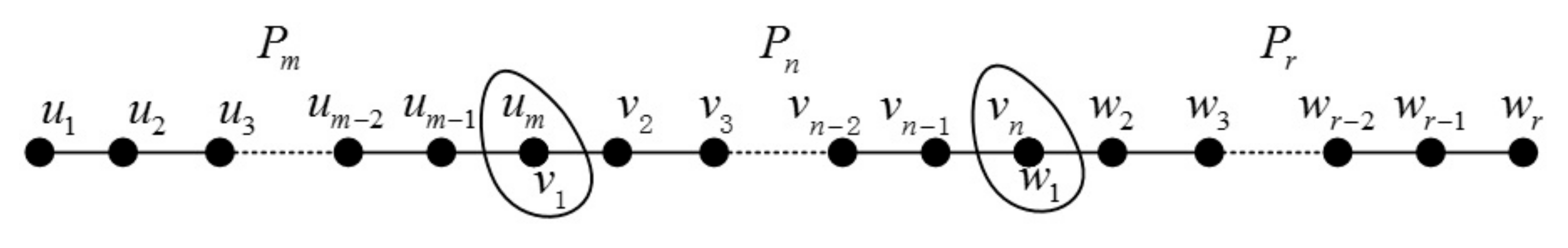
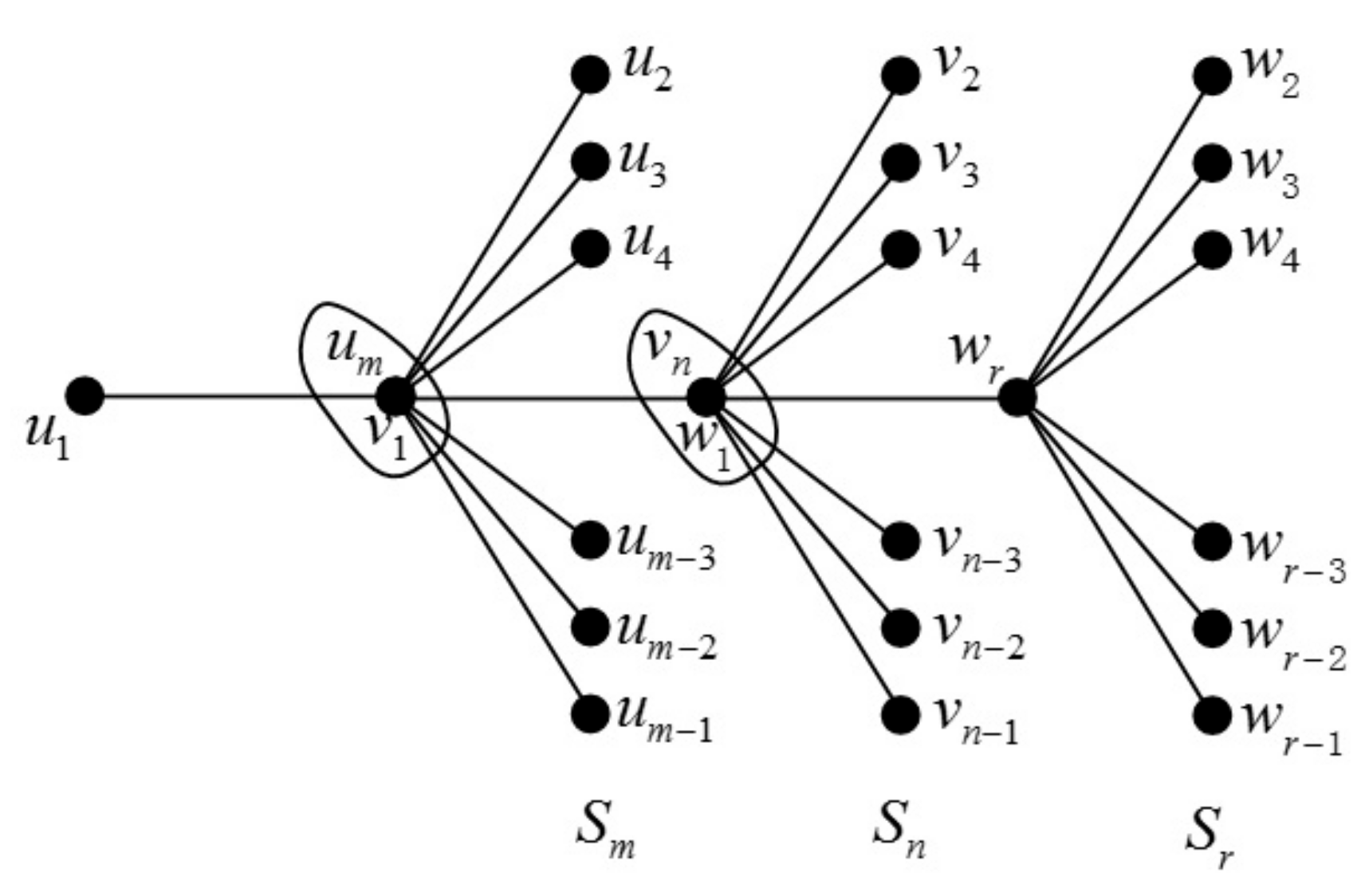
The join graph operation’s definition is given as follows: If we are given two graphs $G$ and $H$ and two vertices $v_i\in V(G)$, $u_j\in V(H)$, the join graph is obtained by merging $v_i$ and $u_j$ into one vertex. The certain join graphs $P_n+C_m$ and $P_n+S_m$ are illustrated in Figure 4 and Figure 5, respectively.

Theorem A is stated in [5]. However, the result is not correct. In this paper, we correct the result of Theorem A and restate it in Theorem 4 as follows:

Theorem A. 

If$n,r\ge 4,m\ge 3$, then

$$AB{C}_e(C_m+P_n+S_r)=\frac{r-2}{2}\sqrt{2r-4}+(r-1)\sqrt{\frac{2r-3}{r(r-1)}}+\frac{\sqrt{2}}{2}(n+m-3)+2$$

(17)

$$G{A}_e(C_m+P_n+S_r)=\frac{2\sqrt{2(r-1)}}{r+1}+(r-1)(\frac{r-2}{2}+\frac{2\sqrt{r(r-1)}}{2r-1})+n+m+\frac{6\sqrt{6}}{5}-4$$

(18)

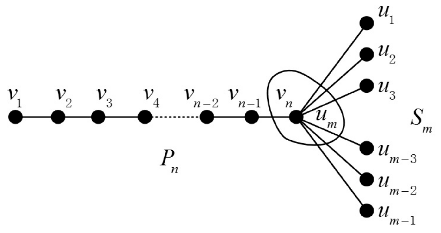
The join graph of $C_m+P_n+S_r$ is illustrated in Figure 6. It can be seen that $d_{L(G)}(v_{n-2}{v}_{n-1})$ is 2 and $d_{L(G)}(v_{n-1}{v}_n)$ is $r$ in $C_m+P_n+S_r$, so we have one edge of types $d_{L(G)}(e)=2$ and $d_{L(G)}(f)=r$ in $G^L(C_m+P_n+S_r)$.

Theorem 4. 

If$n\ge 4,r\ge 4,m\ge 3$, then we have

$$AB{C}_e(C_m+P_n+S_r)=\frac{r-2}{2}\sqrt{2r-4}+(r-1)\sqrt{\frac{2r-3}{r(r-1)}}+\frac{\sqrt{2}}{2}(n+m-3)+2$$

(19)

$$G{A}_e(C_m+P_n+S_r)=\frac{2\sqrt{2r}}{r+2}+(r-1)(\frac{r-2}{2}+\frac{2\sqrt{r(r-1)}}{2r-1})+n+m+\frac{6\sqrt{6}}{5}-4$$

(20)

Proof. 

Let $G=C_m+P_n+S_r$, we have $\left|E_{2,2}^L\right|=n+m-7$, $\left|E_{2,3}^L\right|=3$, $\left|E_{2,r}^L\right|=1$, $\left|E_{3,3}^L\right|=3$, $\left|E_{r-1,r-1}^L\right|=\frac{(r-1)(r-2)}{2}$ and $\left|E_{r-1,r}^L\right|=r-1$.

$$\begin{array}{ll}AB{C}_e(C_m+P_n+S_r)& =(n+m-7)AB{C}_e(E_{2,2}^L)+(3)AB{C}_e^L(E_{2,3})\\ & +(1)AB{C}_e(E_{2,r}^L)+(3)AB{C}_e(E_{3,3}^L)\\ & +\frac{(r-1)(r-2)}{2}AB{C}_e(E_{r-1,r-1}^L)\\ & +(r-1)AB{C}_e(E_{r-1,r}^L)\\ & =(n+m-7)(\sqrt{\frac{2+2-2}{2\times 2}})+(3)(\sqrt{\frac{2+3-2}{2\times 3}})\\ & +(1)(\sqrt{\frac{2+r-2}{2\times r}})+(3)(\sqrt{\frac{3+3-2}{3\times 3}})\\ & +\frac{(r-1)(r-2)}{2}(\sqrt{\frac{(r-1)+(r-1)-2}{(r-1)\times (r-1)}})\\ & +(r-1)(\sqrt{\frac{(r-1)+r-2}{(r-1)\times r}})\\ & =\frac{r-2}{2}\sqrt{2r-4}+(r-1)\sqrt{\frac{2r-3}{r(r-1)}}\\ & +\frac{\sqrt{2}}{2}(n+m-3)+2.\end{array}$$

(21)

Remark: The result of $AB{C}_e(C_m+P_n+S_r)$ is the same as that of [5], only because the $AB{C}_e(E_{2,r-1}^L)=AB{C}_e(E_{2,r}^L)$. We must note $G{A}_e(E_{2,r-1}^L)\ne G{A}_e(E_{2,r}^L)$.

$$\begin{array}{ll}G{A}_e(C_m+P_n+S_r)& =(n+m-7)G{A}_e(E_{2,2}^L)+(3)G{A}_e(E_{2,3}^L)+(1)G{A}_e(E_{2,r}^L)\\ & +(3)G{A}_e(E_{3,3}^L)+\frac{(r-1)(r-2)}{2}G{A}_e(E_{r-1,r}^L)\\ & =(n+m-7)(\frac{2\sqrt{2\times 2}}{2+2})+(3)(\frac{2\sqrt{2\times 3}}{2+3})\\ & +(1)(\frac{2\sqrt{2\times r}}{2+r})+(3)(\frac{2\sqrt{3\times 3}}{3+3})\\ & +\frac{(r-1)(r-2)}{2}(\frac{2\sqrt{(r-1)\times (r-1)}}{(r-1)+(r-1)})\\ & +(r-1)(\frac{2\sqrt{(r-1)\times r}}{(r-1)+r})\\ & =\frac{2\sqrt{2r}}{r+2}+(r-1)(\frac{r-2}{2}+\frac{2\sqrt{r(r-1)}}{2r-1})\\ & +n+m+\frac{6\sqrt{6}}{5}-4.\end{array}$$

(22)

Now the proof is complete.

Theorem 5. 

If$m\ge 2,n\ge 2,r\ge 2$and$P_m+P_n+P_r$be the join graphs depicted in Figure 7, then

$$AB{C}_e(P_m+P_n+P_r)=\frac{\sqrt{2}}{2}(m+n+r-4)$$

(23)

$$G{A}_e(P_m+P_n+P_r)=m+n+r-6+\frac{4}{3}\sqrt{2}$$

(24)

.

Proof. 

Let $G=P_m+P_n+P_r$, we have $\left|E_{2,2}^L\right|=m+n+r-6$ and $\left|E_{1,2}^L\right|=2$.

$$\begin{array}{ll}AB{C}_e(P_m+P_n+P_r)& =(m+n+r-6)AB{C}_e(E_{2,2}^L)+2AB{C}_e(E_{1,2}^L)\\ & =(m+n+r-6)(\sqrt{\frac{2+2-2}{2\times 2}})+2(\sqrt{\frac{1+2-2}{1\times 2}})\\ & =\frac{\sqrt{2}}{2}(m+n+r-4).\end{array}$$

(25)

$$\begin{array}{ll}G{A}_e(P_m+P_n+P_r)& =(m+n+r-6)G{A}_e(E_{2,2}^L)+2G{A}_e(E_{1,2}^L)\\ & =(m+n+r-6)(\frac{2\sqrt{2\times 2}}{2+2})+2(\frac{2\sqrt{1\times 2}}{1+2})\\ & =m+n+r-6+\frac{4}{3}\sqrt{2}.\end{array}$$

(26)

Now the proof is complete.

Theorem 6. 

Let$m\ge 3,r\ge 3,n\ge 6$and$C_m+C_n+C_r$be the join graphs depicted in Figure 8. If$d(u_m,v_n)\ge 3$, then

$$AB{C}_e(C_m+C_n+C_r)=\frac{\sqrt{2}}{2}(m+n+r)-2\sqrt{2}+3\sqrt{6}$$

(27)

$$G{A}_e(C_m+C_n+C_r)=m+n+r+\frac{16\sqrt{2}}{3}$$

(28)

.

Proof. 

Let $G=C_m+C_n+C_r$, we have $\left|E_{2,2}^L\right|=m+n+r-12$, $\left|E_{2,4}^L\right|=8$ and $\left|E_{4,4}^L\right|=12$.

$$\begin{array}{ll}AB{C}_e(C_m+C_n+C_r)& =(m+n+r-12)AB{C}_e(E_{2,2}^L)\\ & +8AB{C}_e(E_{2,4}^L)+12AB{C}_e(E_{4,4}^L)\\ & =(m+n+r-12)(\sqrt{\frac{2+2-2}{2\times 2}})\\ & +8(\sqrt{\frac{2+4-2}{2\times 4}})+12(\sqrt{\frac{4+4-2}{4\times 4}})\\ & =\frac{\sqrt{2}}{2}(m+n+r)-2\sqrt{2}+3\sqrt{6}.\end{array}$$

(29)

$$\begin{array}{ll}G{A}_e(P_m+P_n+P_r)& =(m+n+r-12)G{A}_e(E_{2,2}^L)\\ & +8G{A}_e(E_{2,4}^L)+12G{A}_e(E_{4,4}^L)\\ & =(m+n+r-12)(\frac{2\sqrt{2\times 2}}{2+2})\\ & +8(\frac{2\sqrt{2\times 4}}{2+4})+12(\frac{2\sqrt{4\times 4}}{4+4})\\ & =m+n+r+\frac{16\sqrt{2}}{3}.\end{array}$$

(30)

Now the proof is complete.

Theorem 7. 

Let$m\ge 2,n\ge 3,r\ge 3$and$S_m+S_n+S_r$be the join graphs depicted in Figure 9; then, we have

$$\begin{array}{ll}AB{C}_e(S_m+S_n+S_r)& =(m-1)\sqrt{\frac{2m+n-5}{(m-1)(m+n-2)}}+(n-2)\sqrt{\frac{m+2n-5}{(n-1)(m+n-2)}}\\ & +(n-2)\sqrt{\frac{2n+r-6}{(n-1)(n+r-3)}}+(r-2)\sqrt{\frac{n+2r-7}{(r-2)(n+r-3)}}\\ & +\frac{(m-2)}{2}\sqrt{2m-4}+\frac{(n-2)(n-3)}{2(n-1)}\sqrt{2n-4}+\frac{(r-3)}{2}\sqrt{2r-6}\\ & +\sqrt{\frac{m+2n+r-7}{(m+n-2)(n+r-3)}};\end{array}$$

(31)

$$\begin{array}{ll}G{A}_e(S_m+S_n+S_r)& =2(m-1)\frac{\sqrt{(m-1)(m+n-2)}}{2m+n-3}+2(n-2)\frac{\sqrt{(n-1)(m+n-2)}}{m+2n-3}\\ & +2(n-2)\frac{\sqrt{(n-1)(n+r-3)}}{2n+r-4}+2(r-2)\frac{\sqrt{(r-2)(n+r-3)}}{n+2r-5}\\ & +\frac{(m-1)(m-2)}{2}+\frac{(n-2)(n-3)}{2}+\frac{(r-2)(r-3)}{2}\\ & +\frac{2\sqrt{(m+n-2)(n+r-3)}}{m+2n+r-5}.\end{array}$$

(32)

.

Proof. 

Let $G=S_m+S_n+S_r$, we have $\left|E_{m-1,m+n-2}^L\right|=m-1$, $\left|E_{n-1,m+n-2}^L\right|=n-2$, $\left|E_{n-1,n+r-3}^L\right|=n-2$, $\left|E_{r-2,n+r-3}^L\right|=r-2$, $\left|E_{m-1,m-1}^L\right|=\frac{(m-1)(m-2)}{2}$, $\left|E_{n-1,n-1}^L\right|=\frac{(n-2)(n-3)}{2}$, $\left|E_{r-2,r-2}^L\right|=\frac{(r-2)(r-3)}{2}$ and $\left|E_{m+n-2,n+r-3}^L\right|=1$.

$$\begin{array}{ll}AB{C}_e(S_m+S_n+S_r)& =(m-1)AB{C}_e(E_{m-1,m+n-2}^L)\\ & +(n-2)AB{C}_e(E_{n-1,m+n-2}^L)\\ & +(n-2)AB{C}_e(E_{n-1,n+r-3}^L)\\ & +(r-2)AB{C}_e(E_{r-2,n+r-3}^L)\\ & +\frac{(m-1)(m-2)}{2}AB{C}_e(E_{m-1,m-1}^L)\\ & +\frac{(n-2)(n-3)}{2}AB{C}_e(E_{n-1,n-1}^L)\\ & +\frac{(r-2)(r-3)}{2}AB{C}_e(E_{r-2,r-2}^L)\\ & +(1)AB{C}_e(E_{m+n-2,n+r-3}^L)\\ & =(m-1)\sqrt{\frac{(m-1)+(m+n-2)-2}{(m-1)(m+n-2)}}\\ & +(n-2)\sqrt{\frac{(n-1)+(m+n-2)-2}{(n-1)(m+n-2)}}\\ & +(n-2)\sqrt{\frac{(n-1)+(n+r-3)-2}{(n-1)(n+r-3)}}\\ & +(r-2)\sqrt{\frac{(r-2)+(n+r-3)-2}{(r-2)(n+r-3)}}\\ & +\frac{(m-1)(m-2)}{2}\sqrt{\frac{(m-1)+(m-1)-2}{(m-1)(m-1)}}\\ & +\frac{(n-2)(n-3)}{2}\sqrt{\frac{(n-1)+(n-1)-2}{(n-1)(n-1)}}\\ & +\frac{(r-2)(r-3)}{2}\sqrt{\frac{(r-2)+(r-2)-2}{(r-2)(r-2)}}\\ & +(1)\sqrt{\frac{(m+n-2)+(n+r-3)-2}{(m+n-2)(n+r-3)}}\\ & =(m-1)\sqrt{\frac{2m+n-5}{(m-1)(m+n-2)}}\\ & +(n-2)\sqrt{\frac{m+2n-5}{(n-1)(m+n-2)}}\\ & +(n-2)\sqrt{\frac{2n+r-6}{(n-1)(n+r-3)}}\\ & +(r-2)\sqrt{\frac{n+2r-7}{(r-2)(n+r-3)}}\\ & +\frac{(m-2)}{2}\sqrt{2m-4}+\frac{(n-2)(n-3)}{2(n-1)}\sqrt{2n-4}\\ & +\frac{(r-3)}{2}\sqrt{2r-6}+\sqrt{\frac{m+2n+r-7}{(m+n-2)(n+r-3)}}.\end{array}$$

(33)

$$\begin{array}{ll}G{A}_e(S_m+S_n+S_r)& =(m-1)G{A}_e(E_{m-1,m+n-2}^L)\\ & +(n-2)G{A}_e(E_{n-1,m+n-2}^L)\\ & +(n-2)G{A}_e(E_{n-1,n+r-3}^L)\\ & +(r-2)G{A}_e(E_{r-2,n+r-3}^L)\\ & +\frac{(m-1)(m-2)}{2}G{A}_e(E_{m-1,m-1}^L)\\ & +\frac{(n-2)(n-3)}{2}G{A}_e(E_{n-1,n-1}^L)\\ & +\frac{(r-2)(r-3)}{2}G{A}_e(E_{r-2,r-2}^L)\\ & +(1)AB{C}_e(E_{m+n-2,n+r-3}^L)\\ & =(m-1)\frac{2\sqrt{(m-1)(m+n-2)}}{(m-1)+(m+n-2)}\\ & +(n-2)\frac{2\sqrt{(n-1)(m+n-2)}}{(n-1)+(m+n-2)}\\ & +(n-2)\frac{2\sqrt{(n-1)(n+r-3)}}{(n-1)+(n+r-3)}\\ & +(r-2)\frac{2\sqrt{(r-2)(n+r-3)}}{(r-2)+(n+r-3)}\\ & +\frac{(m-1)(m-2)}{2}\frac{2\sqrt{(m-1)(m-1)}}{(m-1)+(m-1)}\\ & +\frac{(n-2)(n-3)}{2}\frac{2\sqrt{(n-1)(n-1)}}{(n-1)+(n-1)}\\ & +\frac{(r-2)(r-3)}{2}\frac{2\sqrt{(r-2)(r-2)}}{(r-2)+(r-2)}\\ & +(1)\frac{2\sqrt{(m+n-2)(n+r-3)}}{(m+n-2)+(n+r-3)}\\ & =2(m-1)\frac{\sqrt{(m-1)(m+n-2)}}{2m+n-3}\\ & +2(n-2)\frac{\sqrt{(n-1)(m+n-2)}}{m+2n-3}\\ & +2(n-2)\frac{\sqrt{(n-1)(n+r-3)}}{2n+r-4}\\ & +2(r-2)\frac{\sqrt{(r-2)(n+r-3)}}{n+2r-5}\\ & +\frac{(m-1)(m-2)}{2}+\frac{(n-2)(n-3)}{2}\\ & +\frac{(r-2)(r-3)}{2}\\ & +\frac{2\sqrt{(m+n-2)(n+r-3)}}{m+2n+r-5}.\end{array}$$

(34)

Now the proof is complete.

3. Conclusions

The physical and chemical properties of proteins, DNAs and RNAs are very important for human disease and various approaches have been proposed to predict, validate and identify their structures and features [25,26]. Among these, topological indices were proved to be very helpful in testing the chemical properties of new chemical or physical materials such as new drugs or nanomaterials. Topological indices play an important role in studying the topological properties of chemical compounds, especially organic materials i.e., carbon containing molecular structures.

Various topological indices provide a better correlation for certain physico-chemical properties. Hence, the edge version ABC and GA indices for some special Cartesian product graphs and certain join graphs are described by graph structure analysis and a mathematical derivation method in this paper. The results of the current study also have promising prospects for applications in chemical and material engineering. The conclusions we draw here will not work for other classes of indices such as distance-based and distance adjacency-based topological indices. Thus a similar kind of study is needed for other classes of indices which might be a future direction in this area of mathematical chemistry.

References

- Wiener, H. Structural determination of paraffin boiling points. J. Am. Chem. Soc. 1947, 69, 7–20. [Google Scholar] [CrossRef]
- Iranmanesh, A.; Gutman, I.; Khormali, O.; Mahmiani, A. The edge versions of the wiener index. MATCH Commun. Math. Comput. Chem. 2009, 61, 663–672. [Google Scholar]
- Harary, F.; Norman, R.Z. Some properties of line digraphs. Rendiconti del Circolo Matematico di Palermo 1960, 9, 161–169. [Google Scholar] [CrossRef]
- Estrada, E.; Torres, L.; Rodriguez, L.; Gutman, I. An atom-bond connectivity index: Modelling the enthalpy of formation of Alkanes. Indian J. Chem. 1998, 37A, 849–855. [Google Scholar]
- Gao, W.; Farahani, M.; Wang, S.; Husin, M.N. On the edge-version atom-bond connectivity and geometric arithmetic indices of certain graph operations. Appl. Math. Comput. 2017, 308, 11–17. [Google Scholar] [CrossRef]
- Vukicevic, D.; Furtula, B. Topological index based on the ratios of geometric and arithmetical means of end-vertex degrees of edges. J. Math. Chem. 2009, 46, 1369–1376. [Google Scholar] [CrossRef]
- Mahmiani, A.; Khormali, O.; Iranmanesh, A. On the edge version of geometric-arithmetic index. Digest J. Nanomater. Biostruct. 2012, 7, 411–414. [Google Scholar]
- Liu, J.; Pan, X.; Yu, L.; Li, D. Complete characterization of bicyclic graphs with minimal Kirchhoff index. Discrete Appl. Math. 2016, 200, 95–107. [Google Scholar] [CrossRef]
- Liu, J.; Wang, W.; Zhang, Y.; Pan, X. On degree resistance distance of cacti. Discrete Appl. Math. 2016, 203, 217–225. [Google Scholar] [CrossRef]
- Li, X.L.; Shi, Y.T. A survey on the Randic’ index. MATCH Commun. Math. Comput. Chem. 2008, 59, 127–156. [Google Scholar]
- Randić, M. The connectivity index 25 years after. J. Mol. Graph. Modell. 2001, 20, 19–35. [Google Scholar] [CrossRef]
- Ma, J.; Shi, Y.; Wang, Z.; Yue, J. On Wiener polarity index of bicyclic networks. Sci. Rep. 2016, 6, 19066. [Google Scholar] [CrossRef] [PubMed] [Green Version]
- Shi, Y. Note on two generalizations of the Randić index. Appl. Math. Comput. 2015, 265, 1019–1025. [Google Scholar] [CrossRef]
- Estes, J.; Wei, B. Sharp bounds of the Zagreb indices of k-trees. J. Comb. Optim. 2014, 27, 271–291. [Google Scholar] [CrossRef]
- Ji, S.; Wang, S. On the sharp lower bounds of Zagreb indices of graphs with given number of cut vertices. J. Math. Anal. Appl. 2018, 458, 21–29. [Google Scholar] [CrossRef] [Green Version]
- Zafar, S.; Nadeem, M.F.; Zahid, Z. On the edge version of geometric-arithmetic index of nanocones. Stud. Univ. Babes-Bolyai Chem. 2016, 61, 273–282. [Google Scholar]
- Das, K.C.; Trinajstić, N. Comparison between first geometric-arithmetic index and atom-bond connectivity index. Chem. Phys. Lett. 2010, 497, 149–151. [Google Scholar] [CrossRef]
- Furtula, B.; Graovac, A. Atom-bond connectivity index of trees. Discrete Appl. Math. 2009, 157, 2828–2835. [Google Scholar] [CrossRef]
- Fath-Tabar, G.H.; Vaez-Zadeh, B.; Ashrafi, A.R.; Graova, A. Some inequalities for the atom-bond connectivity index of graph operations. Discrete Appl. Math. 2011, 159, 1323–1330. [Google Scholar] [CrossRef]
- Chen, J.; Liu, J.; Guo, X. Some upper bounds for the atom-bond connectivity index of graphs. Appl. Math. Lett. 2012, 25, 1077–1081. [Google Scholar] [CrossRef]
- Das, K.C. Atom-bond connectivity index of graphs. Discrete Appl. Math. 2010, 158, 1181–1188. [Google Scholar] [CrossRef]
- Xing, R.; Zhou, B.; Du, Z. Further results on atom-bond connectivity index of trees. Discrete Appl. Math. 2010, 158, 1536–1545. [Google Scholar] [CrossRef]
- Shao, Z.; Wu, P.; Gao, Y.; Gutman, I.; Zhang, X. On the maximum ABC index of graphs without pendent vertices. Appl. Math. Comp. 2017, 315, 298–312. [Google Scholar] [CrossRef]
- Shao, Z.; Wu, P.; Zhang, X.; Dimitrov, D.; Liu, J. On the maximum ABC index of graphs with prescribed size and without pendent vertices. IEEE Access 2018, 6, 27604–27616. [Google Scholar] [CrossRef]
- Zeng, X.; Lin, W.; Guo, M.; Zou, Q. A comprehensive overview and evaluation of circular RNA detection tools. PLoS Comput. Biol. 2017, 13, e1005420. [Google Scholar] [CrossRef] [PubMed]
- Zeng, X.; Liao, Y.; Liu, Y.; Zou, Q. Prediction and validation of disease genes using HeteSim Scores. IEEE/ACM Trans. Comput. Biol. Bioinform. 2017, 14, 687–695. [Google Scholar] [CrossRef] [PubMed]
Figure 1.
and the line graph of .
Figure 2.
and .
Figure 3.
Figure 4.
The join graph of .
Figure 5.
Figure 6.
Figure 7.
Figure 8.
Figure 9.
Sample Availability: Not available. |
© 2018 by the authors. Licensee MDPI, Basel, Switzerland. This article is an open access article distributed under the terms and conditions of the Creative Commons Attribution (CC BY) license (http://creativecommons.org/licenses/by/4.0/).
Share and Cite
MDPI and ACS Style
Zhang, X.; Jiang, H.; Liu, J.-B.; Shao, Z. The Cartesian Product and Join Graphs on Edge-Version Atom-Bond Connectivity and Geometric Arithmetic Indices. Molecules 2018, 23, 1731. https://doi.org/10.3390/molecules23071731
AMA Style
Zhang X, Jiang H, Liu J-B, Shao Z. The Cartesian Product and Join Graphs on Edge-Version Atom-Bond Connectivity and Geometric Arithmetic Indices. Molecules. 2018; 23(7):1731. https://doi.org/10.3390/molecules23071731
Chicago/Turabian StyleZhang, Xiujun, Huiqin Jiang, Jia-Bao Liu, and Zehui Shao. 2018. "The Cartesian Product and Join Graphs on Edge-Version Atom-Bond Connectivity and Geometric Arithmetic Indices" Molecules 23, no. 7: 1731. https://doi.org/10.3390/molecules23071731