Improving the Accuracy of Density Functional Theory (DFT) Calculation for Homolysis Bond Dissociation Energies of Y-NO Bond: Generalized Regression Neural Network Based on Grey Relational Analysis and Principal Component Analysis

Abstract
:1. Introduction
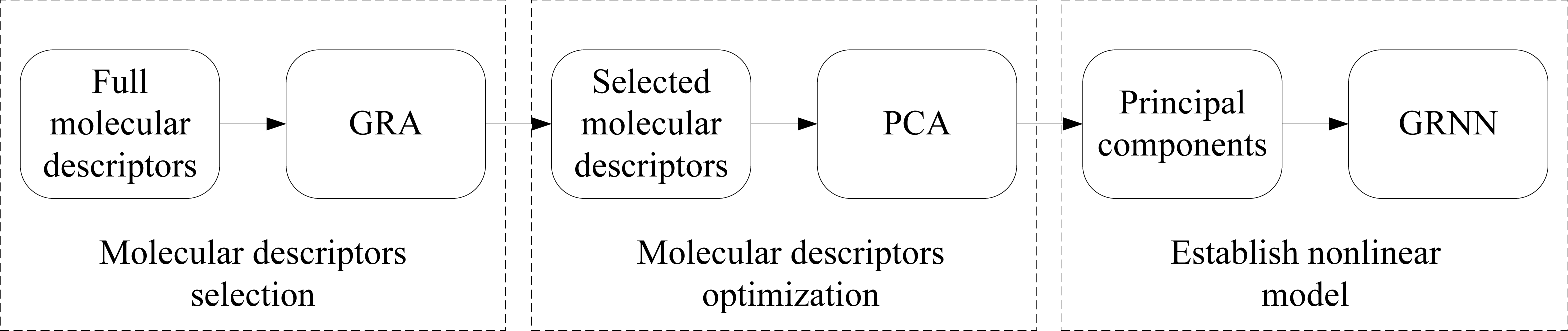
2. Description of Approach
2.1. Grey Relational Analysis
2.2. Principal Component Analysis
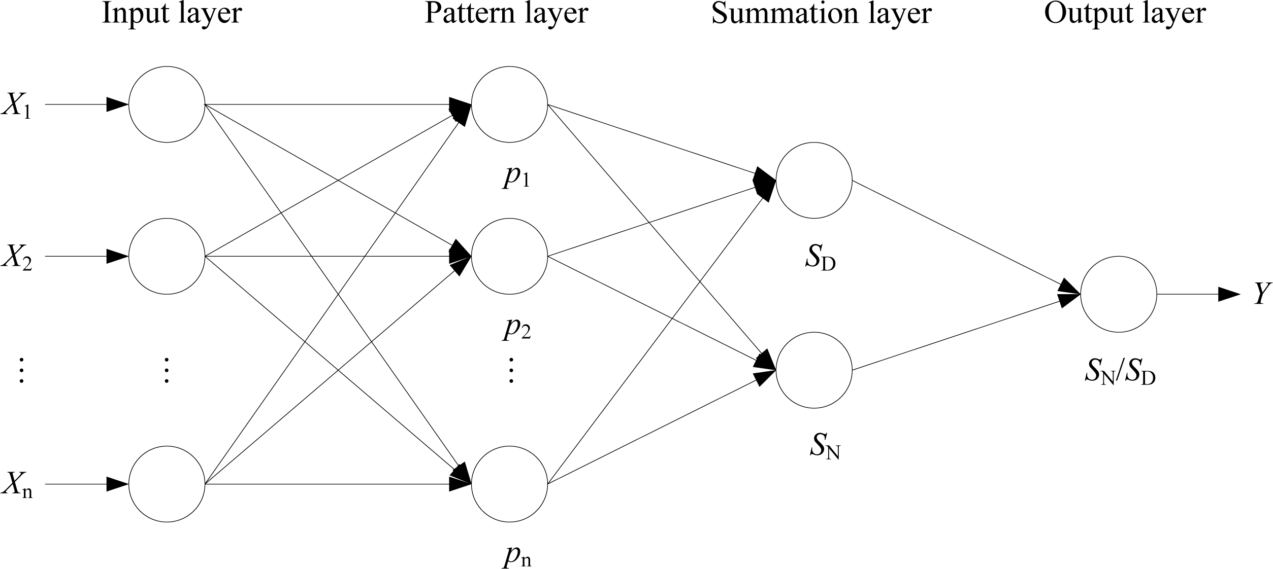
2.3. Generalized Regression Neural Network
3. Computational
3.1. Data Set
3.2. Calculation of Molecular Descriptors
4. Results and Discussion
4.1. Calculation of Descriptor
4.2. Calculation Results of GRA
4.3. Calculation Results of PCA
5. Conclusions
Acknowledgments
References
- Butler, AR; Williams, DLH. The physiological role of nitric oxide. Chem. Soc. Rev 1993, 22, 233–241. [Google Scholar]
- Averill, BA. Dissimilatory nitrite and nitric oxide reductases. Chem. Rev 1996, 96, 2951–2964. [Google Scholar]
- Palmer, RMJ; Ferrige, AG; Moncada, S. Nitric oxide release accounts for the biological activity of endothelium-derived relaxing factor. Nature 1987, 327, 524–526. [Google Scholar]
- Ignarro, LJ. Biosynthesis and metabolism of endothelium-derived nitric oxide. Annu. Rev. Pharmacol. Toxicol 1990, 30, 535–560. [Google Scholar]
- Feldman, PL; Griffith, OW; Stuehr, DJ. The surprising life of nitric oxide. Chem. Eng. News 1993, 71, 26–38. [Google Scholar]
- Fukuto, JM; Ignarro, LJ. In vivo aspects of nitric oxide (NO) chemistry: Does peroxynitrite (OONO) play a major role in cytotoxicity? Acc. Chem. Res 1997, 30, 149–152. [Google Scholar]
- Moncada, S; Palmer, RMJ; Higgs, EA. Nitric oxide: Physiology, pathophysiology, and pharmacology. Pharmacol. Rev 1991, 43, 109–142. [Google Scholar]
- Ignarro, LJ. Signal transduction mechanisms involving nitric oxide. Biochem. Pharmacol 1991, 41, 485–490. [Google Scholar]
- Gnewuch, CT; Sosnovsky, GA. Critical appraisal of the evolution of N-nitrosoureas as anticancer drugs. Chem. Rev 1997, 97, 829–1014. [Google Scholar]
- Cheng, JP; Wang, K; Yin, Z; Zhu, X; Lu, Y. NO affinity. The driving force of nitric oxide (NO) transfer in biomimetic N-nitrosoacetanilide and N-nitrososulfoanilide systems. Tetrahedron Lett 1998, 39, 7925–7928. [Google Scholar]
- Cheng, JP; Xian, M; Wang, K; Zhu, X; Yin, Z; Wang, PG. Heterolytic and homolytic Y-NO bond energy scales of nitroso-containing compounds: Chemical origin of NO release and NO capture. J. Am. Chem. Soc 1998, 120, 10266–10267. [Google Scholar]
- Xian, M; Zhu, XQ; Lu, J; Wen, Z; Cheng, JP. The first O-NO bond energy scale in solution: heterolytic and homolytic cleavage enthalpies of O-nitrosyl carboxylate. Compd. Org. Lett 2000, 2, 265–268. [Google Scholar]
- Zhu, XQ; He, JQ; Li, Q; Xian, M; Lu, J; Cheng, JP. N-NO bond dissociation energies of N-nitroso diphenylamine derivatives (or analogues) and their radical anions: Implications for the effect of reductive electron transfer on N-NO bond activation and for the mechanisms of NO transfer to nitranions. J. Org. Chem 2000, 65, 6729–6735. [Google Scholar]
- Lü, JM; Wittbrodt, JM; Wang, K; Wen, Z; Schlegel, HB; Wang, PG; Cheng, JP. NO affinities of S-nitrosothiols: a direct experimental and computational investigation of RS-NO bond dissociation energies. J. Am. Chem. Soc 2001, 123, 2903–2904. [Google Scholar]
- Zhu, XQ; Hao, WF; Tang, H; Wang, CH; Cheng, JP. Determination of N-NO bond dissociation energies of N-methyl-N-nitrosobenzenesulfonamides in acetonitrile and application in the mechanism analyses on NO transfer. J. Am. Chem. Soc 2005, 127, 2696–2708. [Google Scholar]
- Zhu, XQ; Zhang, JY; Cheng, JP. Mechanism and driving force of NO transfer from S-nitrosothiol to cobalt(II) porphyrin: A detailed thermodynamic and kinetic study. Inorg. Chem 2006, 46, 592–600. [Google Scholar]
- Li, X; Zhu, XQ; Wang, XX; Cheng, JP. Determination of N-NO bond dissociation energies of N-nitrosoindoles and their radical anions in acetonitrile. Chem. J. Chin. Univ 2007, 28, 2295–2298. [Google Scholar]
- Li, X; Zhu, XQ; Cheng, JP. Determination of NO chemical affinities of benzyl nitrite in acetonitrile. Chem. J. Chin. Univ 2007, 29, 2327–2329. [Google Scholar]
- Li, X; Cheng, JP. Determination of S-NO bond dissociation energies of S-nitroso-N-acety-d,l-penicillamine dipeptides. Chem. J. Chin. Univ 2008, 29, 1569–1572. [Google Scholar]
- Li, X; Deng, H; Zhu, XQ; Wang, X; Liang, H; Cheng, JP. Establishment of the C-NO Bond dissociation energy scale in solution and its application in analyzing the trend of NO transfer from C-nitroso compound to thiols. J. Org. Chem 2009, 74, 4472–4478. [Google Scholar]
- Vapnik, VN. Statical Learning Theory; John Wiley&Sons: New York, NY, USA, 1998. [Google Scholar]
- Wang, X; Hu, L; Wong, L; Chen, GH. A combined first-principles calculation and neural networks correction approach for evaluating Gibbs energy of formation. Mol. Simul 2004, 30, 9–15. [Google Scholar]
- Wang, X; Wong, L; Hu, L; Chan, C; Su, ZM; Chen, GH. Improving the accuracy of density-functional theory calculation: the statistical correction approach. J Phys Chem A 2004, 108, 8514–8525. [Google Scholar]
- Duan, XM; Li, ZH; Song, GL; Wang, WN; Chen, GH; Fan, KN. Neural network correction for heats of formation with a larger experimental training set and new molecular descriptors. Chem. Phys. Lett 2005, 410, 125–130. [Google Scholar]
- Balabin, RM; Lomakina, EI; Safieva, RZ. Neural network (ANN) approach to biodiesel analysis: analysis of biodiesel density, kinematic viscosity, methanol and water contents using near infrared (NIR) spectroscopy. Fuel 2011, 90, 2007–2015. [Google Scholar]
- Eros, D; Keri, G; Kovesdi, I; Szantai-Kis, C; Meszaros, G; Orfi, L. Comparison of predictive ability of water solubility QSPR models generated by MLR, PLS, and ANN methods. Mini Rev. Med. Chem 2004, 4, 167–177. [Google Scholar]
- Balabin, RM; Safieva, RZ; Lomakina, EI. Wavelet neural network (WNN) approach for calibration model building based on gasoline near infrared (NIR) spectra. Chemometr. Intell. Lab. Syst 2008, 93, 58–62. [Google Scholar]
- Wu, J; Xu, X. The X1 method for accurate and efficient prediction of heats of formation. J. Chem. Phys 2007, 127, 214105–2141058. [Google Scholar]
- Wu, J; Xu, X. Improving the B3LYP bond energies by using the X1 method. J. Chem. Phys 2008, 129, 164103–164111. [Google Scholar]
- Balabin, RM; Lomakina, EI. Neural network approach to quantum-chemistry data; Accurate prediction of density functional theory energies. J. Chem. Phys 2009, 131, 74104–74108. [Google Scholar]
- Boese, AD; Martin, JML. Development of density functionals for thermochemical kinetics. J. Chem. Phys 2004, 121, 3405–3416. [Google Scholar]
- Hu, L; Wang, X; Wong, L; Chen, GH. Combined first-principles calculation and neural-network correction approach for heat of formation. J. Chem. Phys 2003, 119, 11501–11507. [Google Scholar]
- Li, H; Shi, LL; Zhang, M; Su, ZM; Wang, X; Hu, L; Chen, GH. Improving the accuracy of density-functional theory calculation: The genetic algorithm and neural network approach. J. Chem. Phys 2007, 126, 144101–144108. [Google Scholar]
- Gao, T; Sun, SL; Shi, LL; Li, H; Li, HZ; Su, ZM; Lu, YH. An accurate density functional theory calculation for electronic excitation energies: The least-squares support vector machine. J. Chem. Phys 2009, 130, 184104–184107. [Google Scholar]
- Deng, JL. The theory and method of socioeconomic grey systems. Soc. Sci. China 1984, 6, 47–60. [Google Scholar]
- Deng, JL. Figure on difference information space in grey relational analysis. J. Grey Syst 2004, 16, 96–100. [Google Scholar]
- Huang, SJ; Chiu, NH; Chen, LW. Integration of the grey relational analysis with genetic algorithm for software effort estimation. Eur J. Oper. Res 2008, 188, 898–909. [Google Scholar]
- Jolliffe, IT. Principal Component Analysis; Springer: New York, NY, USA, 1986. [Google Scholar]
- Specht, DF. The general regression neural network-rediscovered. Neural Netw 1993, 6, 1033–1034. [Google Scholar]
- Gaussian 03; Revision B03; Gaussian, Inc: Pittsburgh, PA, USA, 2003.
- Fu, Y; Mou, Y; Lin, BL; Guo, QX. Structures of the X-Y-NO molecules and homolytic dissociation energies of the Y-NO bonds (Y = C, N, O, S). J. Phys. Chem. A 2002, 106, 12386–12392. [Google Scholar]


| No. b | Expt. c | ΔHhomo d | QY | QN | QO | NX | μ | α | EHOMO−1 | EHOMO | ELUMO | ELUMO+1 | ΔE |
|---|---|---|---|---|---|---|---|---|---|---|---|---|---|
| 1 | 43.8 | 26.63 | −0.309 | 0.222 | −0.325 | 87 | 1.83 | 117.55 | −0.2466 | −0.2275 | −0.0744 | −0.0114 | 0.1532 |
| 2 | 36.1 | 28.22 | −0.311 | 0.223 | −0.324 | 79 | 0.91 | 111.89 | −0.2493 | −0.2457 | −0.0761 | −0.0190 | 0.1696 |
| 3 | 38.3 | 28.99 | −0.312 | 0.224 | −0.323 | 71 | 0.46 | 98.39 | −0.2580 | −0.2494 | −0.0781 | −0.0223 | 0.1713 |
| 4 | 37.6 | 28.31 | −0.314 | 0.231 | −0.324 | 87 | 1.53 | 111.82 | −0.2584 | −0.2542 | −0.0855 | −0.0344 | 0.1687 |
| 5 | 39.2 | 29.43 | −0.318 | 0.236 | −0.318 | 93 | 4.54 | 117.63 | −0.2838 | −0.2686 | −0.1039 | −0.0916 | 0.1648 |
| 6 | 34.5 | 25.37 | −0.613 | 0.230 | −0.341 | 145 | 2.81 | 182.34 | −0.2432 | −0.2360 | −0.0556 | −0.0086 | 0.1804 |
| 7 | 35 | 25.99 | −0.614 | 0.231 | −0.340 | 137 | 2.89 | 168.56 | −0.2501 | −0.2397 | −0.0578 | −0.0115 | 0.1819 |
| 8 | 36.2 | 23.67 | −0.627 | 0.251 | −0.336 | 153 | 3.65 | 182.09 | −0.2476 | −0.2432 | −0.0666 | −0.0196 | 0.1766 |
| 9 | 40.4 | 27.27 | −0.615 | 0.239 | −0.332 | 159 | 6.30 | 189.00 | −0.2736 | −0.2582 | −0.0968 | −0.0707 | 0.1614 |
| 10 | 36.2 | 25.30 | −0.614 | 0.234 | −0.338 | 171 | 3.60 | 190.40 | −0.2498 | −0.2425 | −0.0652 | −0.0231 | 0.1773 |
| 11 | 21.4 | 23.56 | −0.247 | 0.213 | −0.368 | 105 | 4.59 | 157.91 | −0.2261 | −0.2146 | −0.0500 | −0.0147 | 0.1646 |
| 12 | 21.4 | 24.10 | −0.248 | 0.214 | −0.366 | 97 | 3.78 | 152.40 | −0.2278 | −0.2213 | −0.0523 | −0.0184 | 0.1690 |
| 13 | 22.6 | 24.32 | −0.250 | 0.216 | −0.365 | 89 | 3.55 | 138.43 | −0.2299 | −0.2248 | −0.0545 | −0.0211 | 0.1702 |
| 14 | 24.1 | 23.71 | −0.252 | 0.220 | −0.361 | 105 | 2.73 | 150.61 | −0.2373 | −0.2318 | −0.0628 | −0.0309 | 0.1690 |
| 15 | 24.3 | 22.74 | −0.256 | 0.226 | −0.353 | 111 | 5.18 | 161.02 | −0.2497 | −0.2437 | −0.0997 | −0.0674 | 0.1440 |
| 16 | 21 | 22.69 | −0.245 | 0.209 | −0.376 | 121 | 5.80 | 178.22 | −0.2209 | −0.2028 | −0.0445 | −0.0135 | 0.1584 |
| 17 | 22.3 | 24.30 | −0.249 | 0.215 | −0.367 | 97 | 3.44 | 151.74 | −0.2281 | −0.2221 | −0.0530 | −0.0193 | 0.1691 |
| 18 | 28.3 | 19.93 | −0.326 | 0.218 | −0.338 | 103 | 3.29 | 136.91 | −0.2379 | −0.2228 | −0.0567 | −0.0045 | 0.1661 |
| 19 | 28.7 | 21.40 | −0.327 | 0.219 | −0.337 | 95 | 2.37 | 131.36 | −0.2430 | −0.2373 | −0.0583 | −0.0077 | 0.1791 |
| 20 | 29.1 | 22.17 | −0.328 | 0.220 | −0.336 | 87 | 2.54 | 117.73 | −0.2507 | −0.2402 | −0.0604 | −0.0108 | 0.1798 |
| 21 | 29.2 | 21.52 | −0.330 | 0.226 | −0.337 | 103 | 3.85 | 131.41 | −0.2511 | −0.2463 | −0.0683 | −0.0225 | 0.1781 |
| 22 | 33.1 | 22.52 | −0.333 | 0.232 | −0.331 | 109 | 6.56 | 137.77 | −0.2664 | −0.2592 | −0.0970 | −0.0752 | 0.1622 |
| 23 | 27.5 | 25.39 | −0.322 | 0.219 | −0.345 | 95 | 2.41 | 128.37 | −0.2449 | −0.2395 | −0.0585 | −0.0139 | 0.1810 |
| 24 | 23.1 | 26.55 | −0.332 | 0.234 | −0.334 | 103 | 1.55 | 127.84 | −0.2527 | −0.2444 | −0.0631 | −0.0253 | 0.1813 |
| 25 | 30.3 | 22.23 | −0.330 | 0.228 | −0.336 | 121 | 4.08 | 137.71 | −0.2481 | −0.2459 | −0.0683 | −0.0235 | 0.1776 |
| 26 | 29.4 | 21.50 | −0.330 | 0.226 | −0.337 | 121 | 3.75 | 139.32 | −0.2492 | −0.2441 | −0.0682 | −0.0230 | 0.1759 |
| 27 | 30.5 | 21.90 | −0.330 | 0.227 | −0.335 | 109 | 3.72 | 147.05 | −0.2515 | −0.2480 | −0.0736 | −0.0553 | 0.1744 |
| 28 | 26.6 | 18.38 | −0.327 | 0.226 | −0.348 | 127 | 3.31 | 174.50 | −0.2394 | −0.2322 | −0.0553 | −0.0030 | 0.1769 |
| 29 | 25.4 | 20.43 | −0.322 | 0.218 | −0.338 | 175 | 2.07 | 247.88 | −0.2389 | −0.2371 | −0.0619 | −0.0130 | 0.1752 |
| 30 | 33.7 | 35.57 | −0.489 | 0.218 | −0.367 | 105 | 5.11 | 128.42 | −0.2500 | −0.2435 | −0.0595 | −0.0395 | 0.1840 |
| 31 | 33.4 | 35.37 | −0.492 | 0.221 | −0.363 | 97 | 5.10 | 122.36 | −0.2690 | −0.2467 | −0.0633 | −0.0466 | 0.1833 |
| 32 | 34.9 | 35.23 | −0.493 | 0.221 | −0.361 | 89 | 4.54 | 108.58 | −0.2783 | −0.2491 | −0.0662 | −0.0499 | 0.1829 |
| 33 | 33 | 34.91 | −0.495 | 0.220 | −0.356 | 105 | 3.11 | 122.51 | −0.2757 | −0.2545 | −0.0730 | −0.0591 | 0.1815 |
| 34 | 33.9 | 34.64 | −0.497 | 0.220 | −0.349 | 111 | 2.00 | 125.62 | −0.2986 | −0.2629 | −0.1125 | −0.0797 | 0.1505 |
| 35 | 33 | 34.92 | −0.495 | 0.221 | −0.356 | 123 | 3.23 | 130.46 | −0.2702 | −0.2542 | −0.0729 | −0.0591 | 0.1813 |
| 36 | 33.7 | 34.32 | −0.501 | 0.228 | −0.349 | 121 | 3.73 | 132.97 | −0.2716 | −0.2568 | −0.0733 | −0.0694 | 0.1835 |
| 37 | 28.7 | 29.86 | −0.219 | 0.233 | −0.355 | 77 | 4.28 | 117.41 | −0.2290 | −0.2198 | −0.0760 | −0.0191 | 0.1438 |
| 38 | 28.6 | 29.36 | −0.221 | 0.235 | −0.351 | 69 | 3.13 | 111.26 | −0.2372 | −0.2276 | −0.0779 | −0.0198 | 0.1497 |
| 39 | 29 | 29.29 | −0.223 | 0.237 | −0.348 | 61 | 2.85 | 97.11 | −0.2465 | −0.2297 | −0.0802 | −0.0233 | 0.1495 |
| 40 | 29.8 | 29.44 | −0.224 | 0.241 | −0.343 | 77 | 2.20 | 111.05 | −0.2467 | −0.2414 | −0.0893 | −0.0360 | 0.1521 |
| 41 | 29.3 | 28.89 | −0.229 | 0.249 | −0.329 | 83 | 4.00 | 116.51 | −0.2715 | −0.2541 | −0.1089 | −0.0828 | 0.1451 |
| 42 | 28.47 | 28.43 | −0.225 | 0.243 | −0.341 | 77 | 3.79 | 110.11 | −0.2569 | −0.2338 | −0.0891 | −0.0356 | 0.1447 |
| 43 | 29.66 | 29.40 | −0.224 | 0.241 | −0.343 | 95 | 2.19 | 119.13 | −0.2433 | −0.2410 | −0.0893 | −0.0360 | 0.1518 |
| 44 | 22.9 | 21.76 | −0.265 | 0.217 | −0.369 | 103 | 3.79 | 155.37 | −0.2333 | −0.2254 | −0.0486 | −0.0139 | 0.1767 |
| 45 | 13.6 | 12.63 | −0.230 | 0.208 | −0.376 | 95 | 3.04 | 143.30 | −0.2346 | −0.2119 | −0.0623 | −0.0231 | 0.1496 |
| 46 | 19.2 | 19.23 | −0.271 | 0.222 | −0.369 | 101 | 3.70 | 165.31 | −0.2299 | −0.2158 | −0.0573 | −0.0476 | 0.1585 |
| 47 | 27.4 | 28.27 | −0.210 | 0.229 | −0.362 | 87 | 3.19 | 142.90 | −0.2329 | −0.2307 | −0.0751 | −0.0406 | 0.1557 |
| 48 | 28.3 | 26.63 | −0.212 | 0.233 | −0.353 | 155 | 0.72 | 189.38 | −0.2452 | −0.2386 | −0.0898 | −0.0596 | 0.1488 |
| 49 | 29.7 | 26.29 | −0.209 | 0.223 | −0.362 | 99 | 3.44 | 152.06 | −0.2377 | −0.2152 | −0.0721 | −0.0161 | 0.1431 |
| 50 | 13.2 | 20.67 | −0.516 | 0.240 | −0.332 | 121 | 5.38 | 156.76 | −0.2605 | −0.2475 | −0.0697 | −0.0523 | 0.1778 |
| 51 | 12.4 | 18.00 | −0.513 | 0.237 | −0.335 | 137 | 6.62 | 176.96 | −0.2454 | −0.2315 | −0.0661 | −0.0483 | 0.1654 |
| 52 | 13.1 | 20.13 | −0.517 | 0.242 | −0.331 | 137 | 4.85 | 171.04 | −0.2594 | −0.2532 | −0.0759 | −0.0586 | 0.1772 |
| 53 | 14.5 | 20.83 | −0.518 | 0.241 | −0.329 | 143 | 3.23 | 186.80 | −0.2584 | −0.2540 | −0.0809 | −0.0706 | 0.1732 |
| 54 | 32.5 | 29.88 | −0.482 | 0.419 | −0.205 | 79 | 4.05 | 111.15 | −0.2672 | −0.2370 | −0.1077 | −0.0420 | 0.1293 |
| 55 | 32.8 | 29.92 | −0.483 | 0.421 | −0.200 | 71 | 3.46 | 103.71 | −0.2637 | −0.2570 | −0.1116 | −0.0490 | 0.1454 |
| 56 | 33.9 | 30.02 | −0.485 | 0.424 | −0.195 | 63 | 2.84 | 89.12 | −0.2682 | −0.2658 | −0.1150 | −0.0522 | 0.1508 |
| 57 | 34.3 | 30.41 | −0.489 | 0.427 | −0.188 | 97 | 1.43 | 111.98 | −0.2795 | −0.2591 | −0.1215 | −0.0619 | 0.1375 |
| 58 | 38.6 | 31.03 | −0.496 | 0.436 | −0.171 | 85 | 2.96 | 107.57 | −0.2964 | −0.2920 | −0.1352 | −0.1074 | 0.1568 |
| 59 | 35 | 30.12 | −0.491 | 0.421 | −0.193 | 31 | 2.09 | 39.15 | −0.3068 | −0.2791 | −0.1159 | 0.0010 | 0.1632 |
| 60 | 37.9 | 30.57 | −0.488 | 0.420 | −0.195 | 39 | 2.04 | 50.08 | −0.3058 | −0.2772 | −0.1146 | 0.0031 | 0.1626 |
| 61 | 36.7 | 29.80 | −0.488 | 0.420 | −0.196 | 47 | 2.14 | 60.61 | −0.3048 | −0.2737 | −0.1142 | 0.0011 | 0.1595 |
| 62 | 33.7 | 40.09 | −0.380 | 0.383 | −0.325 | 73 | 3.67 | 102.43 | −0.2589 | −0.2246 | −0.0688 | −0.0089 | 0.1559 |
| 63 | 33.7 | 37.82 | −0.379 | 0.384 | −0.323 | 65 | 3.06 | 96.97 | −0.2564 | −0.2425 | −0.0706 | −0.0160 | 0.1719 |
| 64 | 35 | 25.04 | −0.380 | 0.385 | −0.322 | 57 | 2.68 | 83.49 | −0.2591 | −0.2515 | −0.0725 | −0.0192 | 0.1790 |
| 65 | 36.2 | 40.39 | −0.382 | 0.388 | −0.318 | 91 | 1.54 | 104.40 | −0.2738 | −0.2482 | −0.0785 | −0.0326 | 0.1698 |
| 66 | 36.2 | 36.75 | −0.388 | 0.394 | −0.308 | 79 | 3.17 | 102.33 | −0.2882 | −0.2792 | −0.0977 | −0.0898 | 0.1815 |
| 67 | 21 | 17.49 | 0.289 | 0.054 | −0.229 | 73 | 3.68 | 111.93 | −0.2520 | −0.2181 | −0.0905 | −0.0398 | 0.1276 |
| 68 | 21.4 | 18.94 | 0.297 | 0.054 | −0.225 | 65 | 2.91 | 105.93 | −0.2532 | −0.2279 | −0.0942 | −0.0439 | 0.1337 |
| 69 | 19.4 | 19.67 | 0.300 | 0.055 | −0.222 | 57 | 2.36 | 91.82 | −0.2556 | −0.2333 | −0.0973 | −0.0465 | 0.1360 |
| 70 | 19.2 | 19.25 | 0.296 | 0.062 | −0.214 | 73 | 0.52 | 106.01 | −0.2618 | −0.2381 | −0.1047 | −0.0568 | 0.1333 |
| 71 | 18.6 | 21.03 | 0.303 | 0.075 | −0.197 | 79 | 3.05 | 113.42 | −0.2737 | −0.2576 | −0.1206 | −0.1006 | 0.1370 |
| 72 | 23.4 | 23.60 | 0.318 | 0.012 | −0.245 | 145 | 2.85 | 221.05 | −0.2407 | −0.2280 | −0.0898 | −0.0303 | 0.1382 |
| 73 | 20.9 | 20.02 | 0.298 | 0.065 | −0.211 | 73 | 2.08 | 104.13 | −0.2624 | −0.2415 | −0.1058 | −0.0575 | 0.1357 |
| 74 | 19.3 | 27.21 | 0.292 | 0.077 | −0.212 | 73 | 3.13 | 102.84 | −0.2606 | −0.2369 | −0.1006 | −0.0593 | 0.1363 |
| 75 | 19.9 | 19.54 | 0.302 | 0.053 | −0.224 | 65 | 2.62 | 104.38 | −0.2536 | −0.2303 | −0.0953 | −0.0443 | 0.1351 |
| 76 | 25 | 27.96 | 0.316 | −0.005 | −0.247 | 49 | 2.76 | 73.43 | −0.2584 | −0.2331 | −0.0887 | −0.0126 | 0.1445 |
| 77 | 17.2 | 18.89 | 0.310 | 0.057 | −0.231 | 73 | 3.50 | 108.44 | −0.2391 | −0.2188 | −0.0870 | −0.0415 | 0.1318 |
| 78 | 24.4 | 27.17 | 0.310 | 0.013 | −0.243 | 179 | 2.14 | 218.16 | −0.2537 | −0.2397 | −0.0944 | −0.0275 | 0.1452 |
| 79 | 24.3 | 26.82 | 0.317 | 0.009 | −0.236 | 161 | 4.93 | 172.55 | −0.2702 | −0.2519 | −0.1066 | −0.0373 | 0.1453 |
| 80 | 26.2 | 27.04 | 0.306 | 0.016 | −0.240 | 171 | 2.49 | 197.57 | −0.2432 | −0.2241 | −0.0977 | −0.0288 | 0.1263 |
| 81 | 26.1 | 27.27 | 0.313 | 0.005 | −0.242 | 131 | 2.22 | 148.15 | −0.2537 | −0.2427 | −0.0974 | −0.0254 | 0.1453 |
| 82 | 26.6 | 27.28 | 0.325 | 0.003 | −0.239 | 163 | 4.86 | 191.09 | −0.2583 | −0.2448 | −0.0994 | −0.0299 | 0.1454 |
| 83 | 29.2 | 27.17 | 0.311 | 0.012 | −0.243 | 163 | 1.57 | 190.12 | −0.2535 | −0.2395 | −0.0942 | 0.0246 | 0.1452 |
| 84 | 27.4 | 27.16 | 0.306 | 0.017 | −0.241 | 139 | 1.23 | 158.73 | −0.2539 | −0.2394 | −0.0939 | −0.0252 | 0.1455 |
| 85 | 28.8 | 21.17 | −0.021 | 0.126 | −0.284 | 79 | 2.14 | 112.96 | −0.2611 | −0.2274 | −0.0916 | −0.0653 | 0.1358 |
| 86 | 29.2 | 24.62 | −0.036 | 0.139 | −0.284 | 85 | 2.66 | 121.41 | −0.2621 | −0.2295 | −0.0946 | −0.0621 | 0.1349 |
| 87 | 27.5 | 20.34 | −0.120 | 0.173 | −0.254 | 117 | 3.29 | 135.55 | −0.2727 | −0.2310 | −0.0915 | −0.0139 | 0.1396 |
| 88 | 27.6 | 19.60 | −0.119 | 0.151 | −0.255 | 109 | 0.96 | 126.38 | −0.2794 | −0.2307 | −0.0931 | −0.0111 | 0.1376 |
| 89 | 26.2 | 22.5 | 0.187 | 0.136 | −0.244 | 69 | 4.52 | 82.90 | −0.2974 | −0.2483 | −0.1097 | −0.0745 | 0.1386 |
| 90 | 30.4 | 19.55 | −0.121 | 0.149 | −0.262 | 101 | 2.94 | 115.49 | −0.2788 | −0.2314 | −0.0927 | −0.0150 | 0.1387 |
| 91 | 31.4 | 22.63 | 0.177 | 0.144 | −0.239 | 47 | 3.99 | 55.09 | −0.3002 | −0.2542 | −0.1127 | −0.0783 | 0.1415 |
| 92 | 26.3 | 17.69 | −0.118 | 0.139 | −0.261 | 61 | 1.77 | 78.22 | −0.2648 | −0.2386 | −0.1020 | −0.0552 | 0.1366 |
| ΔHhomo | QO | NX | α | EHOMO−1 | EHOMO | ELUMO | ΔE | |
|---|---|---|---|---|---|---|---|---|
| ΔHhomo | 1.0000 | −0.0712 | −0.1201 | −0.2483 | −0.3506 | −0.4384 | −0.1329 | 0.2507 |
| QO | 1.0000 | −0.2639 | −0.3599 | −0.5379 | −0.3361 | −0.8101 | −0.6399 | |
| NX | 1.0000 | 0.9331 | 0.3038 | 0.1239 | 0.2756 | 0.2088 | ||
| α | 1.0000 | 0.5355 | 0.3294 | 0.4073 | 0.1729 | |||
| EHOMO−1 | 1.0000 | 0.7963 | 0.7207 | 0.1078 | ||||
| EHOMO | 1.0000 | 0.5695 | −0.2589 | |||||
| ELUMO | 1.0000 | 0.6465 | ||||||
| ΔE | 1.0000 |
| No. | Eigenvalues | Variances (%) | Cumulative (%) |
|---|---|---|---|
| 1 | 3.7039 | 0.4630 | 0.4630 |
| 2 | 1.8642 | 0.2330 | 0.6960 |
| 3 | 1.3980 | 0.1747 | 0.8708 |
| 4 | 0.6259 | 0.0782 | 0.9490 |
| 5 | 0.2211 | 0.0276 | 0.9766 |
| 6 | 0.1573 | 0.0197 | 0.9963 |
| 7 | 0.0296 | 0.0037 | 1.0000 |
| 8 | 0.0000 | 0.0000 | 1.0000 |
| No. | ΔHhomo | QO | NX | α | EHOMO−1 | EHOMO | ELUMO | ΔE |
|---|---|---|---|---|---|---|---|---|
| 1 | −0.1532 | −0.3985 | 0.3084 | 0.3863 | 0.4423 | 0.3413 | 0.4597 | 0.2235 |
| 2 | −0.5035 | −0.3290 | 0.0001 | −0.0929 | −0.2155 | −0.4219 | 0.1850 | 0.6090 |
| 3 | 0.0213 | −0.2076 | −0.6685 | −0.5414 | 0.1997 | 0.3165 | 0.2750 | 0.0294 |
| 4 | 0.8325 | 0.0471 | −0.0684 | −0.0798 | −0.1917 | −0.3043 | 0.0950 | 0.3940 |
| 5 | −0.1589 | 0.7964 | −0.0431 | 0.0081 | 0.4025 | −0.0457 | 0.2491 | 0.3352 |
| 6 | 0.0479 | −0.2266 | −0.2212 | 0.1074 | 0.6798 | −0.4933 | −0.4229 | −0.0391 |
| No. | Expt. a | Deviation b | Deviation c | Deviation d | Deviation e |
|---|---|---|---|---|---|
| 1 | 43.80 | 17.17 | 1.35 | −0.08 | 0.01 |
| 2 | 36.10 | 7.88 | −0.47 | 0.28 | −0.30 |
| 3 | 38.30 | 9.31 | 0.76 | −0.29 | 0.29 |
| 4 | 37.60 | 9.29 | 0.26 | 0.01 | 0.02 |
| 5 | 39.20 | 9.77 | 0.04 | 0.00 | 0.01 |
| 6f | 34.50 | 9.13 | 0.66 | −0.61 | 0.10 |
| 7 | 35.00 | 9.01 | −0.11 | 0.01 | −0.01 |
| 8 | 36.20 | 12.53 | 0.15 | −0.03 | 0.01 |
| 9 | 40.40 | 13.13 | 0.01 | 0.00 | 0.00 |
| 10 | 36.20 | 10.90 | 0.05 | 0.00 | 0.01 |
| 11 | 21.40 | −2.16 | −0.22 | 0.08 | −0.06 |
| 12 | 21.40 | −2.70 | −0.73 | 0.53 | −0.56 |
| 13 | 22.60 | −1.72 | 0.18 | −0.29 | 0.33 |
| 14 | 24.10 | 0.39 | 0.07 | −0.05 | 0.06 |
| 15 | 24.30 | 1.56 | −0.01 | 0.00 | 0.00 |
| 16 | 21.00 | −1.69 | −0.02 | 0.00 | −0.01 |
| 17 | 22.30 | −2.00 | 0.04 | −0.33 | 0.30 |
| 18 | 28.30 | 8.37 | 1.01 | −0.05 | 0.01 |
| 19 | 28.70 | 7.30 | 0.58 | −0.11 | 0.05 |
| 20f | 29.10 | 6.93 | 0.29 | −0.03 | 0.67 |
| 21 | 29.20 | 7.68 | −0.24 | −0.13 | −0.20 |
| 22 | 33.10 | 10.58 | 0.01 | 0.00 | −0.01 |
| 23 | 27.50 | 2.11 | 0.18 | −0.29 | 0.50 |
| 24 | 23.10 | −3.45 | −1.43 | 0.61 | −0.59 |
| 25 | 30.30 | 8.07 | 0.65 | −0.87 | 0.49 |
| 26 | 29.40 | 7.90 | −0.16 | −0.22 | −0.10 |
| 27f | 30.50 | 8.60 | 0.56 | −0.42 | 0.13 |
| 28 | 26.60 | 8.22 | −0.15 | −0.02 | 0.07 |
| 29 | 25.40 | 4.97 | −0.01 | 0.00 | −0.01 |
| 30 | 33.70 | −1.87 | −0.01 | 0.00 | 0.00 |
| 31f | 33.40 | −1.97 | 0.05 | −0.16 | 0.11 |
| 32 | 34.90 | −0.33 | 0.08 | 0.00 | 0.00 |
| 33f | 33.00 | −1.91 | −0.05 | 0.16 | −0.11 |
| 34 | 33.90 | −0.74 | 0.00 | 0.00 | 0.00 |
| 35 | 33.00 | −1.92 | −0.27 | 0.27 | −0.25 |
| 36 | 33.70 | −0.62 | 0.23 | −0.27 | 0.25 |
| 37 | 28.70 | −1.16 | −0.03 | 0.00 | 0.01 |
| 38 | 28.60 | −0.76 | −0.42 | 0.10 | −0.02 |
| 39 | 29.00 | −0.29 | −0.18 | −0.03 | 0.02 |
| 40 | 29.80 | 0.36 | 0.05 | −0.05 | 0.06 |
| 41 | 29.30 | 0.41 | −0.03 | 0.00 | 0.00 |
| 42 | 28.47 | 0.04 | −0.13 | 0.04 | −0.01 |
| 43 | 29.66 | 0.26 | −0.08 | 0.02 | 0.03 |
| 44f | 22.90 | 1.14 | −1.45 | 1.09 | −0.87 |
| 45 | 13.60 | 0.97 | −0.06 | 0.00 | 0.00 |
| 46 | 19.20 | −0.03 | −0.10 | 0.03 | −0.01 |
| 47 | 27.40 | −0.87 | −0.12 | 0.01 | −0.11 |
| 48 | 28.30 | 1.67 | 0.00 | 0.00 | 0.00 |
| 49 | 29.70 | 3.41 | 0.08 | 0.00 | −0.01 |
| 50 | 13.20 | −7.47 | −0.07 | 1.82 | −0.38 |
| 51 | 12.40 | −5.60 | −0.01 | 0.02 | −0.10 |
| 52 | 13.10 | −7.03 | −0.11 | 0.26 | −0.12 |
| 53 | 14.50 | −6.33 | 0.09 | −0.23 | 0.12 |
| 54 | 32.50 | 2.62 | −0.01 | −0.26 | 0.10 |
| 55 | 32.80 | 2.88 | −0.24 | 0.04 | −0.05 |
| 56 | 33.90 | 3.88 | 0.25 | −0.04 | 0.05 |
| 57 | 34.30 | 3.89 | 0.01 | 0.00 | 0.01 |
| 58f | 38.60 | 7.57 | 0.00 | 0.00 | 0.01 |
| 59 | 35.00 | 4.88 | −1.38 | 1.01 | −0.97 |
| 60 | 37.90 | 7.33 | 1.27 | −1.03 | 1.00 |
| 61 | 36.70 | 6.90 | −0.08 | 0.24 | −0.25 |
| 62 | 33.70 | −6.39 | 0.01 | 0.00 | 0.00 |
| 63 | 33.70 | −4.12 | −0.01 | 0.00 | 0.00 |
| 64 | 35.00 | 9.96 | 0.01 | 0.02 | −0.01 |
| 65 | 36.20 | −4.19 | 0.01 | 0.00 | 0.00 |
| 66 | 36.20 | −0.55 | −0.01 | 0.00 | 0.00 |
| 67 | 21.00 | 3.51 | 0.89 | −0.17 | −0.01 |
| 68 | 21.40 | 2.46 | 1.12 | −0.81 | 0.87 |
| 69 | 19.40 | −0.27 | −0.65 | 0.38 | −0.42 |
| 70 | 19.20 | −0.05 | −0.24 | 0.66 | −0.65 |
| 71f | 18.60 | −2.43 | −0.36 | 0.13 | −0.01 |
| 72 | 23.40 | −0.20 | −0.13 | 0.00 | −0.01 |
| 73 | 20.90 | 0.88 | 0.46 | −0.66 | 0.64 |
| 74 | 19.30 | −7.91 | −0.13 | 0.26 | −0.10 |
| 75 | 19.90 | 0.36 | −0.31 | 0.44 | −0.37 |
| 76 | 25.00 | −2.96 | 0.01 | 0.00 | 0.01 |
| 77 | 17.20 | −1.69 | −1.50 | 0.21 | −0.16 |
| 78 | 24.40 | −2.77 | −0.01 | 0.05 | −0.12 |
| 79 | 24.30 | −2.52 | −0.46 | 0.04 | −0.05 |
| 80 | 26.20 | −0.84 | 0.12 | 0.00 | 0.01 |
| 81 | 26.10 | −1.17 | 0.01 | 0.00 | 0.00 |
| 82 | 26.60 | −0.68 | 0.47 | −0.09 | 0.17 |
| 83f | 29.20 | 2.03 | 0.33 | −0.49 | 0.44 |
| 84f | 27.40 | 0.24 | −0.33 | 0.49 | −0.45 |
| 85f | 28.80 | 7.63 | 0.08 | −0.04 | −0.01 |
| 86 | 29.20 | 4.58 | 0.01 | 0.00 | 0.00 |
| 87 | 27.50 | 7.16 | −0.80 | 0.17 | −0.07 |
| 88 | 27.60 | 8.00 | −0.13 | 0.77 | −0.76 |
| 89 | 26.20 | 3.70 | 0.01 | 0.00 | 0.00 |
| 90 | 30.40 | 10.85 | 0.87 | −1.02 | 0.86 |
| 91f | 31.40 | 8.77 | 0.29 | −0.09 | 0.01 |
| 92 | 26.30 | 8.61 | −0.01 | −0.01 | 0.01 |
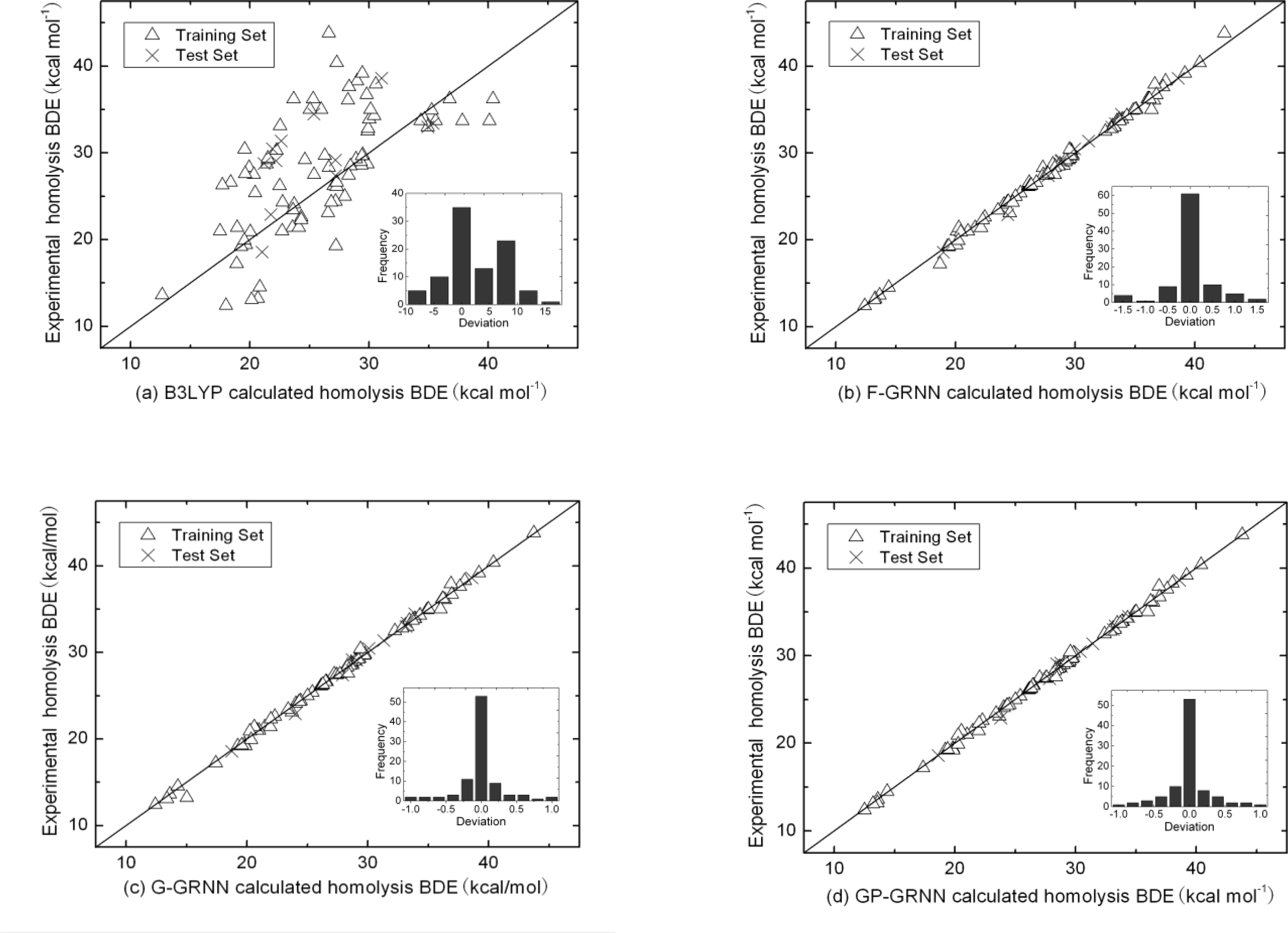
| B3LYP/6-31G (d) | F-GRNN | G-GRNN | GP-GRNN | |
|---|---|---|---|---|
| Training set | 5.40 | 0.48 | 0.38 | 0.30 |
| Test set | 4.69 | 0.55 | 0.46 | 0.39 |
| Overall | 5.31 | 0.49 | 0.39 | 0.31 |
© 2011 by the authors; licensee MDPI, Basel, Switzerland. This article is an open-access article distributed under the terms and conditions of the Creative Commons Attribution license (http://creativecommons.org/licenses/by/3.0/).
Share and Cite
Li, H.Z.; Tao, W.; Gao, T.; Li, H.; Lu, Y.H.; Su, Z.M. Improving the Accuracy of Density Functional Theory (DFT) Calculation for Homolysis Bond Dissociation Energies of Y-NO Bond: Generalized Regression Neural Network Based on Grey Relational Analysis and Principal Component Analysis. Int. J. Mol. Sci. 2011, 12, 2242-2261. https://doi.org/10.3390/ijms12042242
Li HZ, Tao W, Gao T, Li H, Lu YH, Su ZM. Improving the Accuracy of Density Functional Theory (DFT) Calculation for Homolysis Bond Dissociation Energies of Y-NO Bond: Generalized Regression Neural Network Based on Grey Relational Analysis and Principal Component Analysis. International Journal of Molecular Sciences. 2011; 12(4):2242-2261. https://doi.org/10.3390/ijms12042242
Chicago/Turabian StyleLi, Hong Zhi, Wei Tao, Ting Gao, Hui Li, Ying Hua Lu, and Zhong Min Su. 2011. "Improving the Accuracy of Density Functional Theory (DFT) Calculation for Homolysis Bond Dissociation Energies of Y-NO Bond: Generalized Regression Neural Network Based on Grey Relational Analysis and Principal Component Analysis" International Journal of Molecular Sciences 12, no. 4: 2242-2261. https://doi.org/10.3390/ijms12042242