Simple Estimation of Förster Resonance Energy Transfer (FRET) Orientation Factor Distribution in Membranes

Abstract

Because of its acute sensitivity to distance in the nanometer scale, Förster resonance energy transfer (FRET) has found a large variety of applications in many fields of chemistry, physics, and biology. One important issue regarding the correct usage of FRET is its dependence on the donor-acceptor relative orientation, expressed as the orientation factor κ². Different donor/acceptor conformations can lead to κ² values in the 0 ≤ κ² ≤ 4 range. Because the characteristic distance for FRET, R₀, is proportional to (κ²)^1/6, uncertainties in the orientation factor are reflected in the quality of information that can be retrieved from a FRET experiment. In most cases, the average value of κ² corresponding to the dynamic isotropic limit (<κ²> = 2/3) is used for computation of R₀ and hence donor-acceptor distances and acceptor concentrations. However, this can lead to significant error in unfavorable cases. This issue is more critical in membrane systems, because of their intrinsically anisotropic nature and their reduced fluidity in comparison to most common solvents. Here, a simple numerical simulation method for estimation of the probability density function of κ² for membrane-embedded donor and acceptor fluorophores in the dynamic regime is presented. In the simplest form, the proposed procedure uses as input the most probable orientations of the donor and acceptor transition dipoles, obtained by experimental (including linear dichroism) or theoretical (such as molecular dynamics simulation) techniques. Optionally, information about the widths of the donor and/or acceptor angular distributions may be incorporated. The methodology is illustrated for special limiting cases and common membrane FRET pairs.

1. Introduction

Fluorescence spectroscopy has been utilized as a major tool in biophysics in general, and membrane studies in particular, for decades. Several parameters can be measured in steady-state (quantum yield, anisotropy) or time-resolved (intensity and anisotropy decays) conditions, and it allows monitoring of photophysical processes that are sensitive to distance, concentration (Förster Resonance Energy Transfer, FRET), aggregation (FRET, static quenching) or diffusion (collisional quenching). Fluorescence’s versatility and sensitivity have earned it a place among the most useful biophysical techniques [1]. In particular, FRET is a most useful approach to the investigation of diverse problems in membrane biophysics, including membrane protein mapping, lateral heterogeneity (membrane domains), determination of the transverse location (depth) of fluorescent residues/labels inside the membrane, protein/lipid selectivity (preference of a specific lipid for the protein vicinity), and membrane protein oligomerization [2], both in spectroscopic studies and, more recently, under the microscope [3].

Additionally, quantitative applications of membrane fluorescence studies to the recovery of structural and partition information frequently require, as input, results obtained from other techniques. Some of these can be measured experimentally, such as area/lipid, lipid molar volume or bilayer thickness. However, one parameter for which there is no experimental technique suited to a definite measurement (though it was shown by Dale and coworkers that intervals containing it can be inferred from adequate fluorescence anisotropy measurents [4]) is the FRET orientation factor, κ². Because the characteristic distance for FRET, R₀, is proportional to (κ²)^1/6, uncertainties in the orientation factor are reflected on the quality of information that can be retrieved from a FRET experiment. Most often, the theoretical value for the so-called dynamic isotropic limit (<κ²> = 2/3) is used, but <κ²> uncertainty is still widely regarded as an inconvenience [5] that may be especially important in membranes, because of their intrinsic anisotropic nature and the restricted rotational mobility experienced by fluorophores incorporated inside the bilayer. The 2/3 value corresponds to the dynamic limit, where rotation of both donor and acceptor is fast compared with the excited state lifetime.

As described in detail below in Section 3.1., the instant value of κ² for a given donor-acceptor pair (which falls in the 0 ≤ κ² ≤ 4 range) can be calculated from adequate molecular frame vectors. Although this definition of κ² is not suited to experimental measurement, it can be conveniently used in molecular simulation studies. In particular, from the instant position coordinates of a molecular dynamics (MD) simulation trajectory, calculation of the orientation factor for a given FRET donor-acceptor molecular pair is straightforward, and averaging both over pairs and over time is conveniently carried out. This has been used in a number of literature reports (e.g., [6–9]) including membrane-embedded fluorophores [10]. However, this approach is not a choice for most experimental researchers, as setup and validation of MD simulations for novel fluorophores (for which parameterization is seldom available) is not trivial.

Even though computational calculations of κ² are scarce, determination of membrane-embedded fluorophore orientations using computational (for reviews of MD studies of fluorescent membrane probes, see [11,12]) or experimental techniques (traditionally linear dichroism or other spectroscopic methods [13,14], or, more recently, methods based on polarized total internal reflection fluorescence microscopy or other microscopic techniques [15–17]) are more frequent.

This manuscript describes a simple manner to use data on probe location and orientation or alignment in membranes, obtained by experimental or molecular simulation methods, to provide estimates for the κ² distribution in the dynamic limit, from numerical simulation. For this purpose, a simple program was developed to generate random planar location distributions of donor and acceptor probes. Fluorophore orientation is then generated for each donor or acceptor taking into account information provided by the user. Subsequently, κ² is calculated for a large number of donor/acceptor pairs, and hence the κ² distribution and average value are obtained. Average κ² values for common membrane FRET pairs were obtained and are shown. For other FRET applications, the reader may use the software, which is available as supporting information to this article, without difficulty. This simplified approach enables immediate estimation of κ² distributions for quantitative FRET applications, without the need to resort to sophisticated theoretical or experimental techniques.

2. Results and Discussion

2.1. Special Theoretical Cases

This manuscript describes a simple manner to use data on probe orientation or alignment in membranes to estimate the distribution of the κ² FRET factor, using a small program described in more detail in Section 3. In this subsection we use the program to verify some results known from the literature, as well as to investigate other hypothetical scenarios of interest.

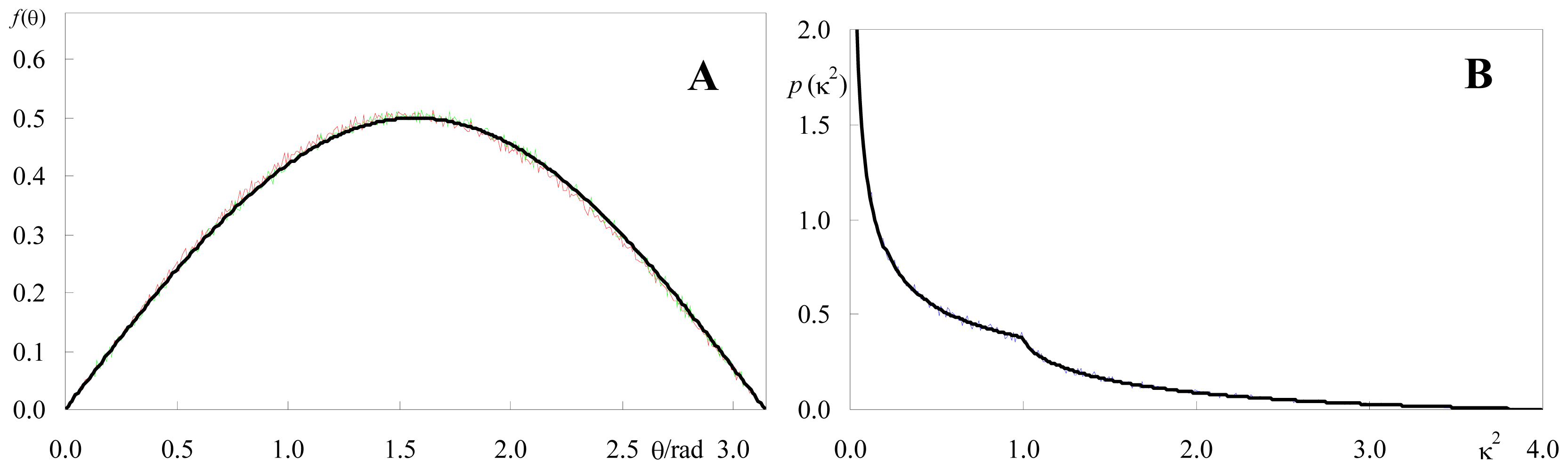
2.1.1. Isotropic Dipole Distribution

As described in Section 3, the software assumes normal distributions of cosθ_D and cosθ_A (truncated to the range −1 ≤ cosθ ≤ 1), where θ_D and θ_A are the tilts of donor and acceptor (respectively) relative to the normal to the membrane plane. The angles corresponding to the distribution maxima are read, as well as the standard deviations σ_A and σ_B. If very wide angular distributions are used (σ >> 1) uniform azimuth angular distributions f(θ) = sinθ/2 are in practice obtained, as illustrated in Figure 1A. Therefore, and because ϕ distribution is uniform in the [0, 2π] interval, isotropic orientation of both donor and acceptor is easily simulated.

Figure 1B shows the resulting probability density of κ² compared with the analytical result for isotropic dipoles, which is (e.g., [5]):

$$p({\kappa }^2)=\{\begin{array}{ll}\frac{1}{2\sqrt{3{\kappa }^2}}\text{ln}(2+\sqrt{3})\hfill & 0\le {\kappa }^2\le 1\hfill \\ \frac{1}{2\sqrt{3{\kappa }^2}}\text{ln}\left(\frac{2+\sqrt{3}}{\sqrt{{\kappa }^2}+\sqrt{{\kappa }^2-1}}\right)\hfill & 1\le {\kappa }^2\le 4\hfill \end{array}$$

(1)

From the density distribution, one can calculate the average value,

$$\langle {\kappa }^2\rangle =\underset{0}{\overset{4}{\int }}{\kappa }^{2}p({\kappa }^2)d{\kappa }^2=2/3$$

(2)

As shown in Figure 1B, there is excellent agreement between both simulated and analytical distributions and average κ² value. The result <κ²> = 2/3, described in the literature [18] for planar probe distribution, is identical to that for isotropic orientation of dipoles distributed in a three dimensional system. The latter can also be obtained from the program, with a slight modification for the position of the acceptor in each pair (allowing a randomly allocated acceptor z value—varying e.g., between 0 and a maximal value specified by the user—in each donor-acceptor pair). Again, there is excellent agreement with the theoretical expectations (not shown).

2.1.2. Identical or Identically-Distributed Fluorophores

This situation is illustrated in the inset of Figure 2. In this case, the distribution and average value of κ² for planar systems depend solely on the angle θ_D between the donor transition dipole and the normal to the membrane plane. An analytical solution to this situation was described by Knoester and van Himbergen [19], who showed that

$$\langle {\kappa }^2\rangle =\frac{2}{3}-\frac{2}{3}S+S^2$$

(3)

where

$$S=\frac{3\langle {\text{cos}}^2\hspace{0.17em}{\theta }_D\rangle -1}{2}$$

(4)

is an orientation order parameter, equal to the average value of the second-order Legendre polynomial P₂(θ). For this particular case, since no orientation heterogeneity is (as yet) assumed, <cosθ_D> = cosθ_D. This result, which arguably is little known in the membrane fluorescence research community, is however very pertinent e.g., for FRET among identical fluorophores (energy migration, energy transfer or homo-FRET).

Figure 2 shows that the variation of <κ²> against θ_D, obtained using our numerical approach, agrees with the analytical result. Large relative variations are observed, and between local maxima for θ_D = 0 (<κ²> = κ² (invariant) = 1), 90° (<κ²> = 1.25) and 180° (<κ²> = κ² (invariant) = 1), there are minima (<κ²> = 5/9) at θ_D = acos((5/9)^1/2) = 41.81° and 180° – 41.81° = 138.19°. There are four θ_D values for which an average of 2/3 is obtained. These values correspond to the angles in the [0, 180°] interval for which S = 0 ↔ cosθ_D = ± (1/3)^1/2 (the so-called magic angle 54.74°, and 125.26°) and S = 2/3 ↔ cosθ_D = ± (7/9)^1/2 (28.13°, 151.87°). However, despite <κ²> being identical to the isotropic value, the κ² distributions are quite different. As shown in Figure 3, the κ² distribution for θ_D = 54.74° shows peaks at κ² ≈ 0.12 and κ² ≈ 1 (absent in the isotropic distribution), while it vanishes abruptly for κ² > 25/9 = 2.778. This latter higher limiting value corresponds to the situation of coplanar donor dipole, acceptor dipole and separation vector, with the two dipoles facing each other. On the contrary, in the isotropic limit, values of κ² near 4 (corresponding to collinear dipoles) are allowed and no cutoff is observed.

To illustrate the utility of this curve for quick estimation of <κ²>, we consider the recent MD study of 1-palmitoyl,2-[12-amino]dodecanoyl-sn-glycero-3-phosphocholine (C12-NBD-PC) in a fluid bilayer of 1,2-dipalmitoyl-sn-3-glycerophoshocholine (DPPC, T = 323 K). The angular distribution of the transition dipole has a maximum around ~120–125° relative to the bilayer normal [20]. From Figure 2, this would be consistent with <κ²> = 0.67–0.77. Direct calculation of κ² using the atomic coordinates of the MD trajectory leads accordingly to <κ²> = 0.72 ± 0.04 for molecules in the same-leaflet [10].

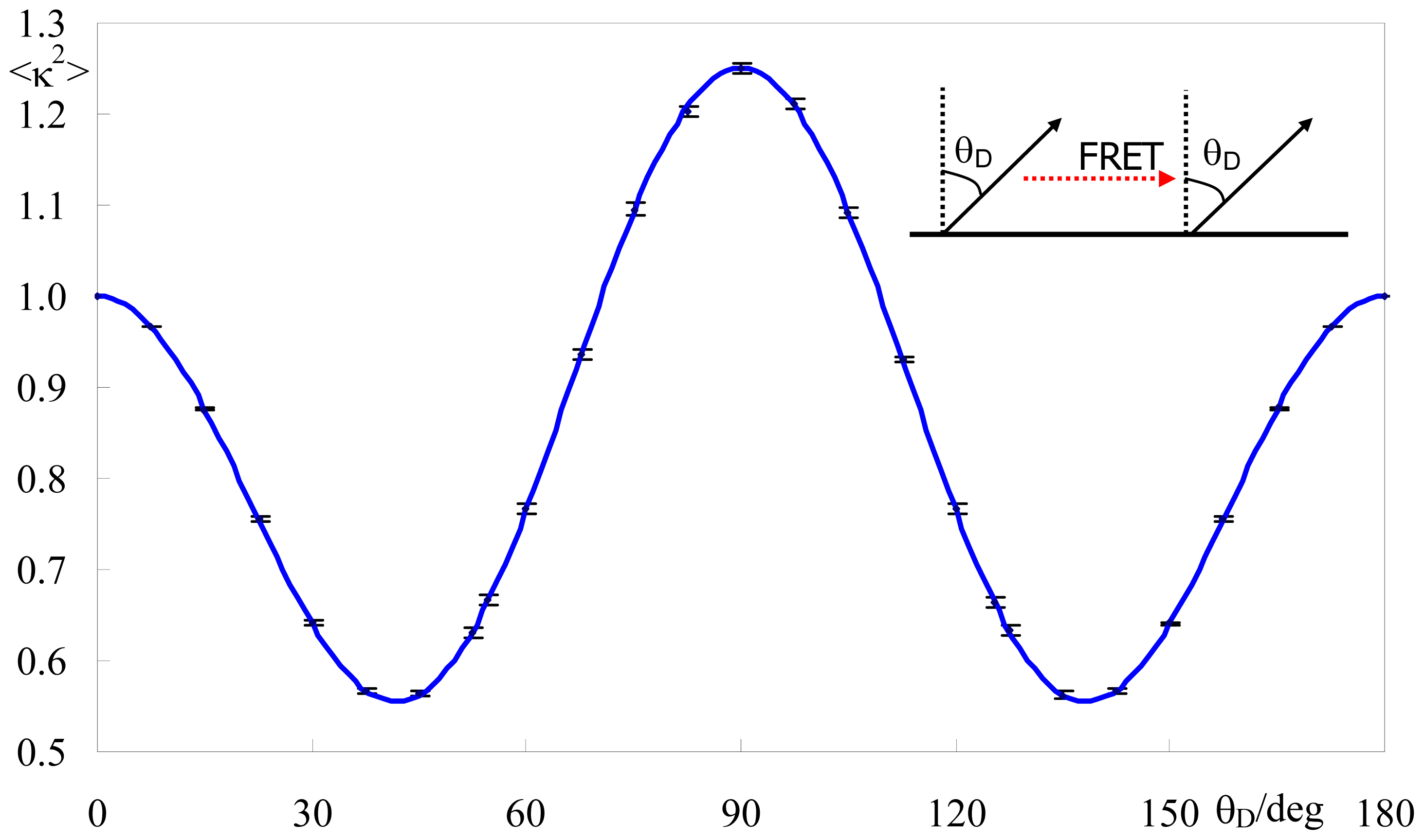
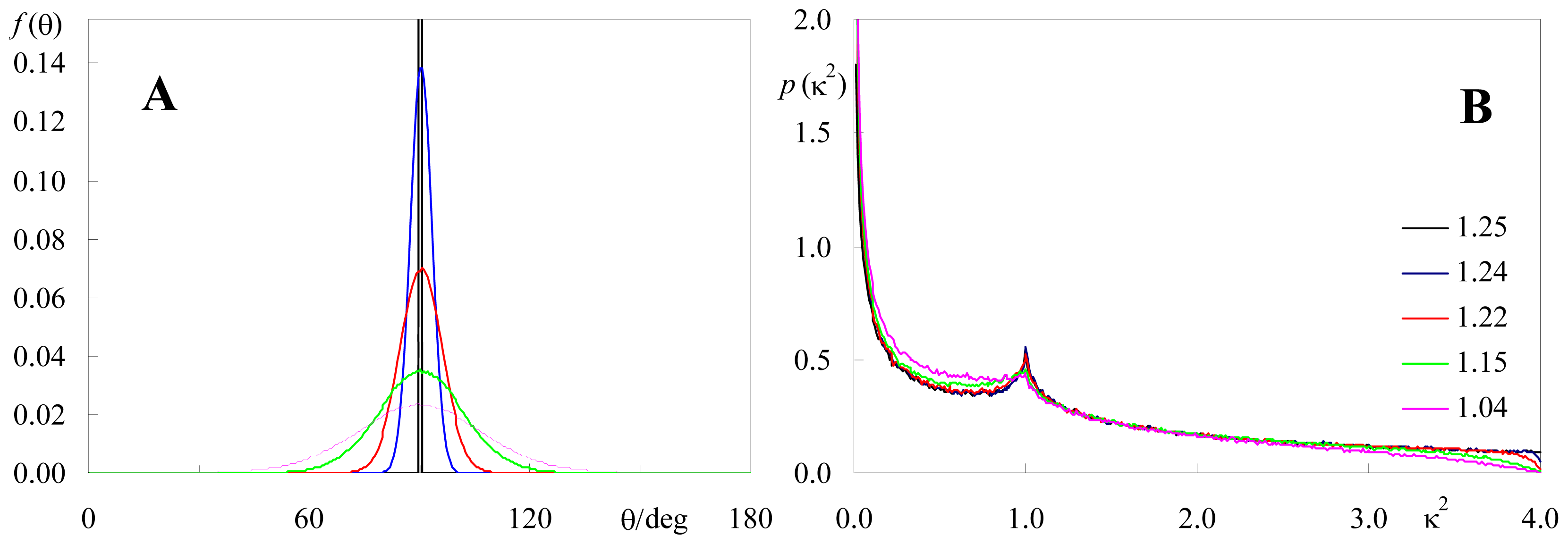
2.2. Effect of Orientation Heterogeneity

One important feature of our numerical procedure for estimation of κ² distributions of membrane-embedded fluorophores is that it allows the introduction of orientation heterogeneity, in the form of a normal distribution of cosθ_D and/or cosθ_A, as mentioned previously. This type of heterogeneity is expected in simple rotational models such as the “wobbling-in-cone” motions [21]. The standard deviations of the cosθ_D and cosθ_A distributions (σ_D and σ_A, respectively) are a measure of the extent of freedom of dipole orientation. Therefore, they serve a similar purpose to that of Dale et al.’s depolarization factors <d_D^x> and <d_A^x> [4]: σ and <d^x> are different ways to express the orientation distributions sampled by donor and acceptor. Whereas Dale et al.’s form of taking this orientation redistribution into account using depolarization factors was justified by their perceived possibility of estimation of <κ²> ranges from time-resolved fluorescence polarization measurements, σ is a technique-independent, more direct metric of the dipole orientation heterogeneity.

Intuitively, upon permitting sampling of different donor/acceptor relative orientations, κ² distributions and average values are necessarily affected. As discussed above, the limiting case of σ >> 1 leads to the expected isotropic case. Here we address the more physical possibility of moderate heterogeneity (σ ≈ 0.05–0.3) and its effect upon the orientation factor. Figures 4 and 5 illustrate the alterations produced on κ² distributions and average values upon widening the angular distributions of donor and acceptor dipoles for two distinct situations: identical donor and acceptor distributions (e.g., homo-FRET) centered around θ = 90° (Figure 4) and quite distinct donor and acceptor distributions centered around 60° and 120°, respectively (Figure 5). In these calculations, a larger number of pairs (at least 10⁶) should be considered, to allow a better sampling of the θ_D and θ_A distributions. In both cases, it can be seen that whereas moderate orientation heterogeneity produces visible alterations in κ² distribution, significant effects require a very large degree of heterogeneity. This is more apparent for the system where donor and acceptor have very distinct angular distributions (Figure 5), where, remarkably, very wide distributions of both probes affect κ² by a degree <10%.

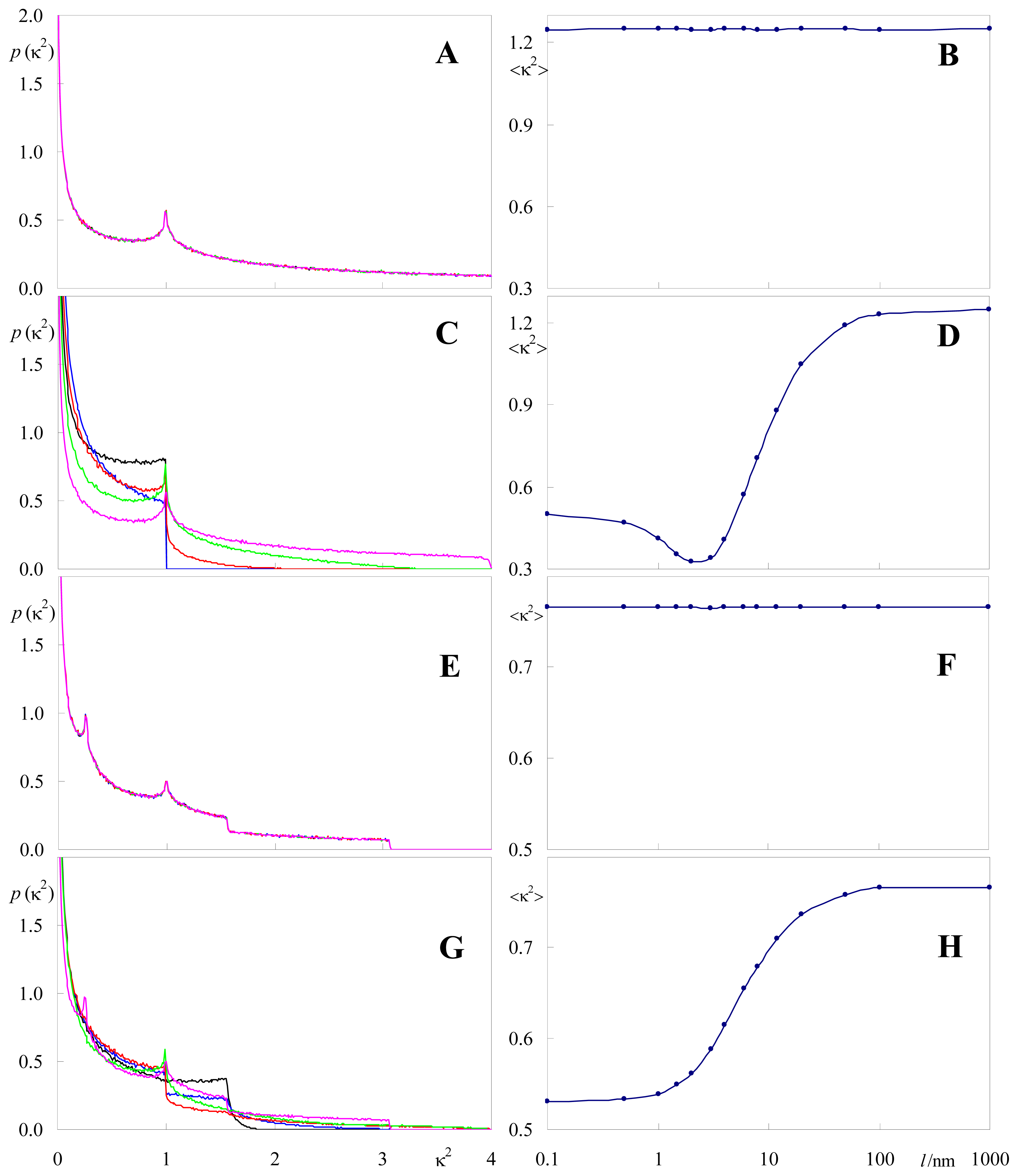
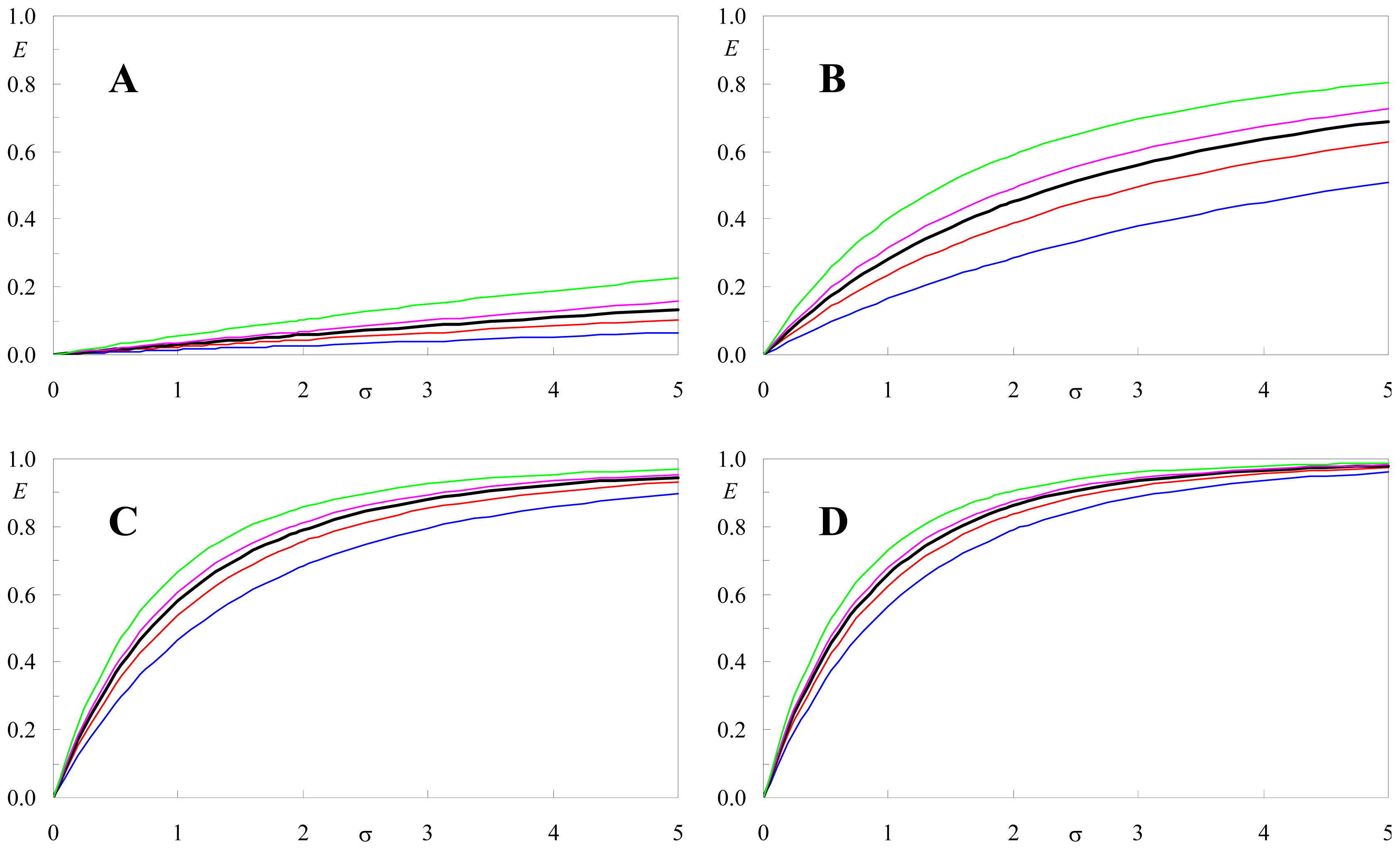
2.3. Distance Effects

In most applications of intramolecular FRET (involving a single acceptor fluorophore as quencher of each donor), distance measurements are carried out assuming a single fixed value of R₀, assuming a <κ²> value (usually 2/3) independent of donor-acceptor distance. However, this view has been challenged, as MD simulations revealed considerable correlation between κ² and donor-acceptor distance in a labeled protein [6], possibly related to constraints imposed by the linker used to attach the donor probe. Naturally, in systems where each donor may transfer its excitation energy to multiple acceptors at varying distances, correlation between donor-acceptor distance and their relative orientation will necessarily occur if the dynamic isotropic limit is not met. Consider for example that donors and acceptors are located in separate parallel planes (different depths in the membrane), and that both types of fluorophores have narrow orientation distribution. The range and relative weight of possible κ² values will certainly differ for a donor-acceptor pair in which the acceptor is located directly below or above the donor, relative to the case where their lateral separation is large. Therefore, the question is not whether there exists correlation, but to which extent κ² may vary as a function of distance, and how to best take this into account.

For the sake of illustration, we consider the same donor and acceptor orientations as in the previous subsection, but assuming fixed (no orientation heterogeneity) θ_D = θ_A = 90° and (θ_D, θ_A) = (60°, 120°). We also consider two separate possibilities in each case: (i) coplanar donor and acceptor spatial distributions; (ii) donor and acceptor planes separated by an arbitrary distance of h = 2.0 nm. In each of these scenarios, the size of the square systems l was varied up to 1000 nm. 10⁶ pairs were simulated for proper sampling of donor/acceptor distances. It is clear from the figure that location of both donor and acceptor dipoles in the same plane always lead to identical distributions (Figure 6A,E) and average values (Figure 6B,F). At variance, for donors and acceptors placed in parallel planes, there are very significant changes in both κ² distribution (Figure 6C,G) and <κ²> (Figure 6D,H), when the size of the simulated system (which constraints the maximal possible donor-acceptor distance) is <<100 nm.

In this case, definition of an average κ² becomes a problem. The best way to deal with this situation is to take notice of how FRET occurs from a given donor (with fluorescence lifetime in absence of acceptor equal to τ₀) to a distribution of M acceptors (where the distance between the selected donor and the ith-acceptor is denoted by R_i). The decay rate k is given by

$$k={\tau }_0^{-1}+k_T={\tau }_0^{-1}+\sum _{i=1}^M{k}_i$$

(3)

where the different individual FRET rates are calculated according to

$$k_i=\frac{1}{{\tau }_0}{\left(\frac{R_{0i}}{R_i}\right)}^6$$

(4)

Finally, the Förster radius for each donor-acceptor pair is calculated using

$$R_{0i}=0.02108{\left[{\kappa }_i^2{\mathrm{\Phi }}_0{n}^{-4}\underset{0}{\overset{\infty }{\int }}{\lambda }^{4}I(\lambda )\varepsilon (\lambda )d\lambda \right]}^{1/6}$$

(5)

where Φ₀ is the quantum yield of the donor in the absence of acceptor molecules, n is the refractive index of the medium, and the integral term is the overlap between the normalized donor emission (I(λ)) and the acceptor absorption (ɛ(λ)) spectra. The constant value in the equation above assumes nm units for both λ and R₀, as well as M⁻¹cm⁻¹ units for ɛ(λ). Combining these three equations, one concludes that the FRET rate is given by

$$k_T=C\sum _{i=1}^M\frac{{\kappa }_i^2}{R_i^6}$$

(6)

where C is a constant term for all acceptors in the distribution. That is, the natural way to average κ² over different acceptors, with different distances to a given donor, is to use the inverse sixth power of the donor-acceptor distance as weight. In this way, acceptors located more closely contribute significantly more to the average (as they are also responsible for most of the quenching by FRET). For the purpose of this calculation, we adapted our program for averaging κ² in this way for FRET between a plane of donors and another of acceptors, and FRET in a bilayer geometry (with possibility of FRET between a plane of donors and two planes of acceptors—one in each bilayer leaflet). We then proceeded to calculate <κ²> for the two angular distributions presented above (θ_D = θ_A = 90°; and (θ_D, θ_A) = (60°, 120°)) assuming a bilayer geometry with h₁ = 0.0 and h₂ = 2.0 nm as the donor-acceptor interplanar distances. For coplanar fluorophores, an exclusion distance of R_e = 0.8 nm was also introduced, as donors and acceptors in the same plane cannot lie closer than a given minimum distance value. This would be similar to a typical experiment, with acceptor distribution in both bilayer leaflets. For a better sampling of all possible orientations for small R_i values, a value of l = 100 nm was used. Ten different simulations were carried out in each case, to assess whether proper convergence was obtained. For θ_D = θ_A = 90°, an average of 1.237 with standard deviation 0.010 was obtained, whereas for (θ_D, θ_A) = (60°, 120°) the corresponding values were 0.771 and 0.009. The relatively small standard deviations indicate that sampling was adequate. The average values were similar (very slightly lower) to the <κ²> calculated for the planar systems (1.250 and 0.776, respectively), and the small differences are due to the contribution of acceptors lying in the opposite leaflet. Because of the transverse distance of 2 nm, neglecting this leaflet does not lead to considerable error. In any case, for the following section that applies this methodology to computation of <κ²> for common experimental donor-acceptor pairs, whenever possible, information on donor-acceptor interplanar distances was taken into account.

2.4. Application to Experimental FRET Pairs

Table 1. Donor and acceptor location and orientation literature data for common FRET pairs in membranes, and <κ²> calculated from this information.

Donor fluorophore a	Acceptor fluorophore a	Quantitative experimental FRET studies	Donor transverse location b	Donor orientation (θmax, σ) c	Acceptor transverse location	Acceptor orientation (θmax, σ) c	Calculated <κ2> d
t-PnA	DPH	[24,25]	0.92 nm [26]e	20°, 0.15 f	0.75 nm [27]f	0, 0.35 [27]f	0.58 ± 0.01
DPH	NBD	[28–31]	0.75 nm [27]f	0, 0.35 [27]f	1.35 nm [20,32,33]e,f	125°, 0.35 [20]f	0.66 ± 0.01
NBD	NBD	[34,35]	1.35 nm [20,32,33]f	125°, 0.35 [20]f	1.35 nm [20,32,33]e,f		0.66 ± 0.03
NBD	Carbocyanine	[36]			1.26 nm [37]f	77°, 0.25 [37]f	0.76 ± 0.02
NBD	Rhodamine B	[25,35,38–42]			2.1 nm [43,44]f	90°, 0.275 [43,45]g	0.56 ± 0.02
BODIPY	Rhodamine B	[30,46]	0.8 nm [47]f	10°, 0.5 [47]f			0.57 ± 0.01
BODIPY	Carbocyanine	[48]			1.26 nm [37]f	77°, 0.25 [37]f	0.72 ± 0.02
Rhodamine B	Rhodamine B	[25,35,41,49,50]	2.1 nm [43,44]f	90°, 0.275 [43,45]g	2.1 nm [43,44]f	90°, 0.275 [43,45]g	1.08 ± 0.01

^at-PnA: trans-parinaric acid; DPH: diphenylhexatriene; NBD: 7-nitrobenz-2-oxa-1,3-diazol-4-yl)amino; BODIPY: 4,4-difluoro-3a,4adiaza-s-indacene;

^bRelative to the center of the bilayer;

^cThe values given refer to the θ_max and σ values (read by the simulation program) that produce angular distributions most consistent with the simulation or experimental data reported in the cited references;

^dAverage and standard deviations of average for ten independent simulations with two planes, R_i⁻⁶ weight, N = 10⁶, R_e = 0.8 nm and l = 100 nm;

^eInferred from experimental fluorescence quenching data;

^fInferred from simulation data;

^gInferred from linear dichroism data.

summarizes relevant information regarding membrane probes that are commonly involved in FRET experiments (as donors, acceptors or both), Förster pair combinations formed by these probes, examples of quantitative experimental FRET studies using these pairs, and information obtained from literature simulation or experimental studies regarding fluorophore location and transition dipole orientation of the probes. The latter information was used to calculate an average κ² value using the inverse sixth power of the donor-acceptor distance as weight, as described in the previous subsection. These averages are also shown in the Table. It can be seen that all these values but one (homo-FRET between Rhodamine B probes) lie within 15% or 0.1 of the isotropic limit of 2/3, even though the probe orientation distributions are quite varied. The most probable explanation for this is that all orientation data retrieved from the literature refer to liquid disordered bilayers, in which probes have generally broad angular distributions. Applications to FRET in liquid ordered or gel phases, where conformational freedom is largely reduced, would potentially lead to <κ²> further from the 2/3 value. This is illustrated in the t-PnA/DPH pair. For t-PnA, contrary to other probes, information regarding orientation distribution is also available in the gel phase (5°, 0.03 (gel) [22]). Using these input values instead of the fluid phase parameters, one would obtain <κ²> = 0.53 ± 0.01 instead of 0.58 ± 0.01 for both probes in the fluid phase. It should also be emphasized that the dipole orientation details shown in Table 1 refer to a specific probe compound labelled with the fluorophore under consideration, and other probes exist where the same fluorophore could be expected to show different transverse location and/or orientation distribution in the bilayer. For example, NBD data are based in a MD study of NBD-PC, whereas FRET studies also employ other NBD probes (NBD-PE, NBD-cholesterol).

2.5. Effect of <κ²> on FRET Efficiency

The most common experimental observables in FRET are the decay of donor in the presence of acceptor, i_DA(t), and the FRET efficency, E. The decay law i_DA(t) for bilayer geometries and uniform probe distribution is available in the literature [23]

$$i_{DA}(t)=\text{exp}\left(-\frac{t}{{\tau }_0}\right)\text{exp}\left\{-\pi R_0^{2}c\gamma \left[\frac{2}{3},{\left(\frac{R_0}{R_e}\right)}^6\left(\frac{t}{{\tau }_0}\right)\right]{\left(\frac{t}{{\tau }_0}\right)}^{1/3}\right\}·\text{exp}\left\{\pi R_e^{2}c\left(1-\text{exp}\left[-{\left(\frac{R_0}{R_e}\right)}^6\left(\frac{t}{{\tau }_0}\right)\right]\right)\right\}$$

(7)

In this equation, c is the number of acceptors per unit area, γ is the incomplete gamma function, and the other symbols have the same meaning as in the previous equations. Although Equation 7 was originally derived for a plane of acceptors containing the donor (cis transfer), it is also valid if the donor molecule is separated from the acceptor plane by a distance R_e. From the time-resolved donor emission, the FRET efficiency, which is defined (and often experimentally measured) by

$$E=1-I_{DA}/I_D$$

(8)

(where I_DA and I_D are the donor steady-state emission intensities in presence and absence of donor, respectively), can be calculated using

$$E=1-\underset{0}{\overset{\infty }{\int }}{i}_{DA}(t)dt/\underset{0}{\overset{\infty }{\int }}{i}_D(t)dt$$

(9)

In the latter equation, i_D(t) = exp(-t/τ₀) is the donor time-resolved fluorescence decay in the absence of acceptor.

To appreciate the effect of <κ²> on the FRET efficiency, we first define $\overline{R_0}$ as the value of the Förster radius calculated with κ² = 2/3, and then consider a form of Equation 7 in terms of dimensionless parameters ζ= t/τ₀ (reduced time), $\sigma =\pi {\overline{R_0}}^{2}c$ (number of acceptors in a circle of radius equal to $\overline{R_0}$), $\alpha =\overline{R_0}/R_{\text{e}}$ and β = (3/2)<κ²>:

$$i_{DA}(\varsigma )=\text{exp}(-\varsigma )\text{exp}\left\{-{\beta }^{1/3}\sigma \left(\gamma \left[\frac{2}{3},\beta {\alpha }^6\varsigma \right]{\varsigma }^{1/3}-\frac{1-\text{exp}\left(-\beta {\alpha }^6\varsigma \right)}{{\beta }^{1/3}{\alpha }^2}\right)\right\}$$

(10)

This form of the decay law is suitable for calculation (by integration over ζ, done using Equation 9 after substitution of variables t and ζ) of universal curves E vs. σ, for fixed values of α and β. Representative examples are shown in Figure 7.

From Figure 7, it can be seen that variations in FRET efficiency upon changing the <κ²> value used to calculate R₀ are most important when the latter is smaller than or comparable to the exclusion distance, such as in panels (a) and (b). For example, for $\alpha =\overline{R_0}/R_{\text{e}}=0.50$, the FRET efficiency obtained for <κ²> = 1.25 is >3 times larger than that obtained for for <κ²> = 0.30 over the whole σ < 5 range. However, it must be noted that larger values of $\alpha =\overline{R_0}/R_{\text{e}}$ are often met in membranes, as long as R₀ has a reasonable (~2.5 nm or larger) value and there are acceptors in the same bilayer leaflet as the donors. In these cases, such as illustrated in panels (c) and (d), the effect of <κ²> on E, though still clearly detectable, is smaller, especially in the 0.50 < <κ²> < 0.80 range which is observed for most common FRET pairs (Table 1).

3. Methods

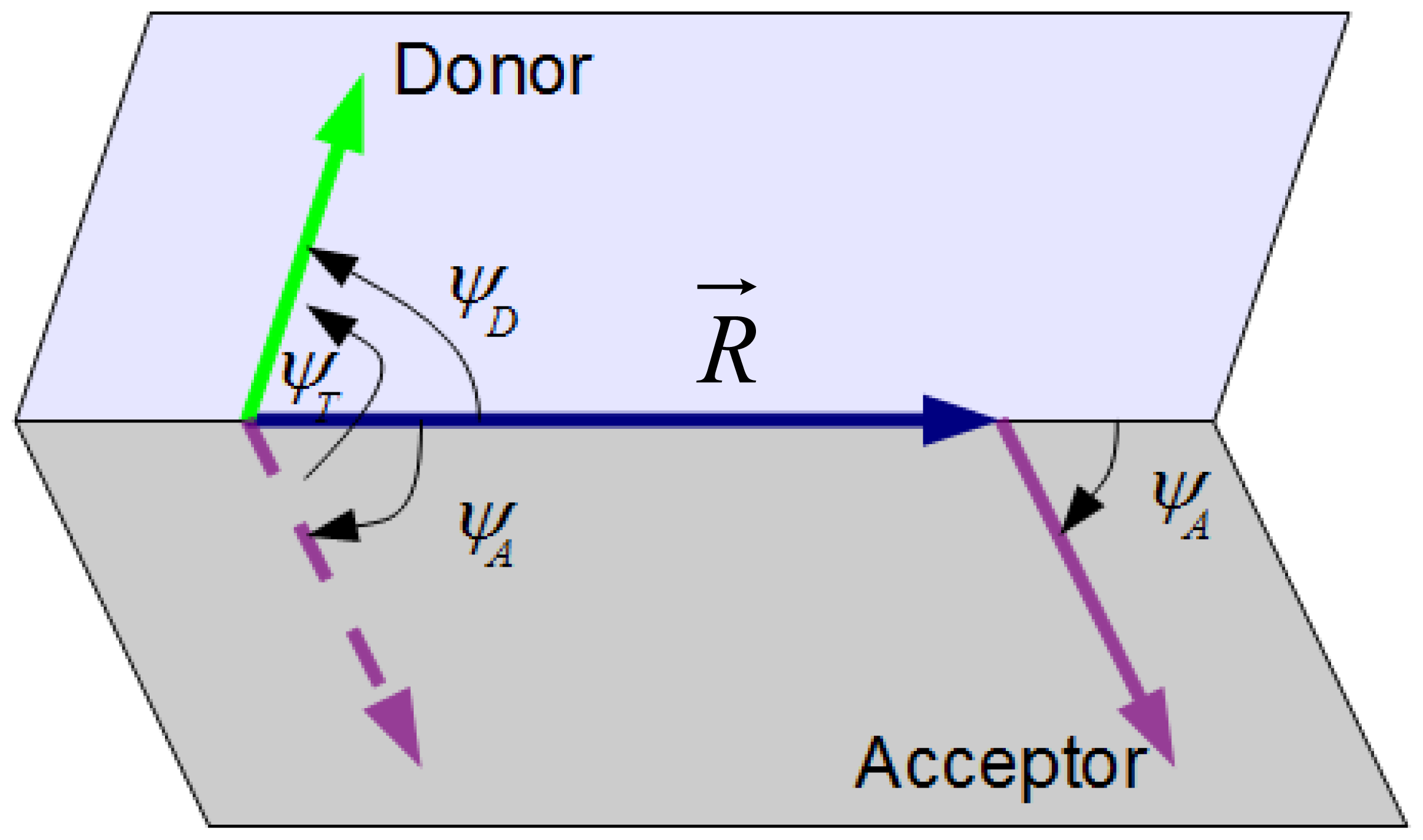
3.1. Definition of κ² for a Given Donor-Acceptor Pair

κ² is given by [5]

$${\kappa }^2={(\text{cos}{\psi }_T-3\hspace{0.17em}\text{cos}{\psi }_D\hspace{0.17em}\text{cos}{\psi }_A)}^2$$

(11)

where Ψ_T is the angle between the transition moments of the donor and acceptor and Ψ_D and Ψ_A are the angles between the donor and acceptor transition moments and the vector uniting their centers, R⃗ (Figure 8). An equivalent expression, involving scalar products of &rrarr; = R⃗/||R⃗|| and unit vectors &urarr;_D and &urarr;_A (in the direction of the donor and acceptor dipoles, respectively), is

$${\kappa }^2={\left({\overrightarrow{u}}_D·{\overrightarrow{u}}_A-3(\overrightarrow{r}·{\overrightarrow{u}}_D)(\overrightarrow{r}·{\overrightarrow{u}}_A)\right)}^2$$

(12)

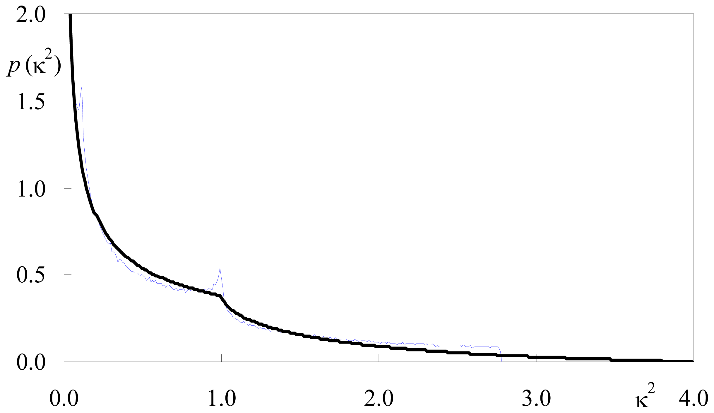
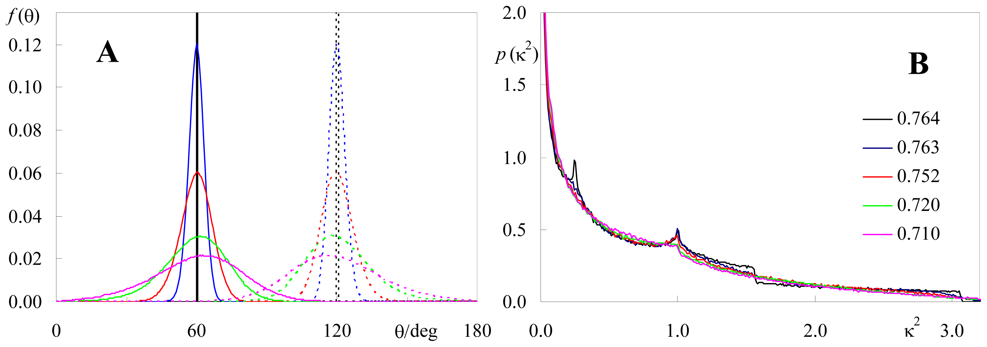
3.2. Calculation of κ² Distributions and Averages from Numerical Simulation

Two programs, written as macros in the Visual Basic Editor within a Microsoft Excel document, were developed for this article. The programs are available as supplemental files to this article, and may be edited by any user. Microsoft Excel Visual Basic was chosen as it may be easily used by most readers, and produces immediate numerical and graphic output.

Program 1 calculates κ² distributions and average values without weighting, for a single acceptor plane. The basic algorithm can be summarized as follows:

• Read inputs: θ_D,max, θ_A,max, σ_D, σ_A, l, N, donor-acceptor interplanar distance h, and the number of bins (equal length subintervals of 0 ≤ κ² ≤ 4) for κ² distribution.
• Main cycle – calculate κ² for the i^th donor-acceptor pair:
  • 2.1. Set donor and acceptor coordinates, (x_Di, y_Di, z_Di) and (x_Ai, y_Ai,z_Ai), respectively. For the x and y-coordinates, uniformly distributed random numbers between 0 and L are allotted. z_Di is taken as zero, whereas z_Ai is taken as h.
  • 2.2. Calculate donor-acceptor separating vector R⃗, and its modulus.
  • 2.3. Set donor and acceptor dipole orientation coordinates, (θ_Di, ϕ_Di) and (θ_Ai, ϕ_Ai), respectively. For ϕ_Di and ϕ_Ai, uniformly distributed random numbers between 0 and 2π are allotted. θ_Di and θ_Ai (the angles relative to the bilayer normal, so that they fall between 0 and π) are calculated by firstly computing their cosines, using Gaussian random numbers centered around cosθ_D,max and cosθ_A,max, with standard deviation σ_D and σ_A, respectively. Gaussian random numbers are obtained using the Box-Muller transform method [51,52]. If either of the calculated cosines falls outside the [-1,1] interval, new cosθ_Di and cosθ_Ai are calculated. Otherwise, θ_Di and θ_Ai are obtained in the [0, π] interval by inversion.
  • 2.4. Calculate Cartesian coordinates of unit dipole vectors u⃗_D and u⃗_A, from (θ_Di, ϕ_Di) and (θ_Ai, ϕ_Ai).
  • 2.5. Calculate κ² using Equation 12.
  • 2.6. Update histogram of κ² distribution (in fact, the program also calculates θ_D and θ_A distributions, for testing and/or comparison and matching with distributions from the literature; these are also updated at this point), and partial sum of κ² values (for calculation of <κ²> = sum(κ²_i)/N at the end of the cycle).
  • 2.7 Increment i and repeat until i > N.
• Write outputs to the active worksheet: κ² average value and distribution, θ_D and θ_A distributions.

All calculations and distributions shown in Figures 1–6 were obtained with this program.

Program 2 follows a similar algorithm for calculation of κ² for the i^th donor-acceptor pair. However, it computes an average κ² value using R_i⁻⁶ as weight for each pair. It may be used for both one and two acceptor planes. The program reads θ_D,max, θ_A,max, σ_D, σ_A, l, N, and, for both planes, the respective donor-acceptor interplanar (h₁ and h₂) and exclusion (R_e1 and R_e2) distances. Two main cycles are carried out, one for each acceptor plane, with calculation of κ² distribution in each case. For both cycles, calculation of κ² for the i^th donor-acceptor pair is identical to that in the first program, with an additional check: if R_i < R_e1 (first cycle) or R_i < R_e2 (second cycle), then new donor and acceptor distance coordinates are allotted and a corresponding new R_i is calculated. Partial sums of κ²/R⁶ values are now computed, to obtain <κ²> = sum(κ²_i/R_i⁶)/sum(1/R_i⁶). As described in Section 3, this weighting scheme reflects the dependence of the FRET interaction with distance, and was used to compute the values of the right column of Table 1 (see footnote for typical input parameters).

4. Conclusions

A simple method for calculation of the distribution and average value of the FRET orientation factor κ², for membrane-located donor and acceptor fluorophores, is presented. The method is implemented in two programs that are available with the present article. The programs use as inputs the donor and acceptor transverse locations, orientation and orientational heterogeneity. Analytical results previously obtained in limiting cases were verified, validating our approach. A number of donor/acceptor orientation distributions tested in this work produce κ² distributions and average values which are significantly different to that corresponding to the isotropic limit, characterized by <κ²> = 2/3. Considerable dependence of <κ²> on system size l when the latter is <<100 nm was verified, which presents a problem regarding the most appropriate <κ²> to consider for the purpose of quantitative analysis of FRET data. It is proposed that calculating <κ²> using the sixth inverse power of the donor-acceptor distance is the most natural way to average κ² in this situation, and estimates of <κ²> were obtained for common membrane FRET pairs using available fluorophore location and orientation data. It was shown that for most of these systems, the calculated <κ²> lies within ±15% of the 2/3 value, possibly because probes in fluid bilayers have very broad orientation distributions. In these cases, substantial effects on FRET efficiency are not expected, provided that the Förster radius is significantly larger than the donor-acceptor exclusion distance. For more ordered bilayers, narrow orientation distributions may produce <κ²> further form the 2/3 value. In these ordered systems, an additional problem is that fluorophore dipole orientation randomization may occur in a time scale of the order or slower than the donor excited state lifetime. In case reorientation proceeds much slower than transfer, the opposite regime (static limit) is operative. As discussed in detail elsewhere [4,5], in this limit, it is generally not possible to use κ² averages to calculate donor-acceptor distances in intramolecular FRET (the only exceptions occur for isotropic dipole distribution or when the FRET efficiency is vanishingly small). In the intermediate case of comparable rates of reorientation and transfer, FRET kinetics becomes very complex [19]. Because these situations of restricted mobility are not contemplated in our method, which calculates κ² distributions and averages corresponding to the dynamic limit, care must be taken when addressing these systems. However, even in such cases, the ease of application of this method—as long as fluorophore location and orientation data (or, at worst, “educated guesses”) are available (in the literature or upon measurement) for the pair at hand—allows calculation of <κ²> which will constitute an improvement over the widely used but very seldom justified <κ²> = 2/3 assumption.

References

1. Lakowicz, J.R. Principles of Fluorescence Spectroscopy, 3rd ed; Springer: New York, NY, USA, 2006. [Google Scholar]
2. Loura, L.M.S.; Prieto, M. FRET in membrane biophysics: An overview. Front Physiol 2011, 2, 82. [Google Scholar]
3. De Almeida, R.F.; Loura, L.M.S.; Prieto, M. Membrane lipid domains and rafts: Current applications of fluorescence lifetime spectroscopy and imaging. Chem. Phys. Lipids 2009, 157, 61–77. [Google Scholar]
4. Dale, R.E.; Eisinger, J.; Blumberg, W.E. The orientational freedom of molecular probes. The orientation factor in intramolecular energy transfer. Biophys. J 1979, 26, 161–193. [Google Scholar]
5. Van der Meer, B.W. Kappa-squared: From nuisance to new sense. Rev. Mol. Biotechnol 2002, 82, 181–196. [Google Scholar]
6. VanBeek, D.B.; Zwier, M.C.; Shorb, J.M.; Krueger, B.P. Fretting about FRET: Correlation between κ and R. Biophys. J 2007, 92, 4168–4178. [Google Scholar]
7. Allen, L.R.; Paci, E. Orientational averaging of dye molecules attached to proteins in Förster resonance energy transfer measurements: Insights from a simulation study. J. Chem. Phys 2009, 131, 065101. [Google Scholar]
8. Hoefling, M.; Lima, N.; Haenni, D.; Seidel, C.A.M.; Schuler, B.; Grubmüller, H. Structural heterogeneity and quantitative FRET efficiency distributions of polyprolines through a hybrid atomistic simulation and Monte Carlo approach. PLoS One 2011, 6, e19791. [Google Scholar]
9. Deplazes, E.; Jayatilaka, D.; Corry, B. Testing the use of molecular dynamics to simulate fluorophore motions and FRET. Phys. Chem. Chem. Phys 2011, 13, 11045–11054. [Google Scholar]
10. Loura, L.M.S.; Palace Carvalho, A.J.; Prates Ramalho, J.P. Direct calculation of Förster orientation factor of membrane probes by molecular simulation. J. Mol. Struct. THEOCHEM 2010, 946, 107–112. [Google Scholar]
11. Loura, L.M.S.; Prates Ramalho, J.P. Fluorescent membrane probes’ behaviour in lipid bilayers: Insights from molecular dynamics simulations. Biophys. Rev 2009, 1, 141–148. [Google Scholar]
12. Loura, L.M.S.; Prates Ramalho, J.P. Recent developments in molecular dynamics simulations of fluorescent membrane probes. Molecules 2011, 16, 5437–5452. [Google Scholar]
13. Hicks, M.R.; Kowałski, J.; Rodger, A. LD spectroscopy of natural and synthetic biomaterials. Chem. Soc. Rev 2010, 39, 3380–3393. [Google Scholar]
14. Lopes, S.C.D.N.; Castanho, M.A.R.B. Overview of common spectroscopic methods to determine the orientation/alignment of membrane probes and drugs in lipidic bilayers. Curr. Org. Chem 2005, 9, 889–898. [Google Scholar]
15. Oreopoulos, J.; Yip, C.M. Probing Membrane order and topography in supported lipid bilayers by combined polarized total internal reflection fluorescence-atomic force microscopy. Biophys. J 2009, 96, 1970–1984. [Google Scholar]
16. Beausang, J.F.; Sun, Y.; Quinlan, M.E.; Forkey, J.N.; Goldman, Y.E. Orientation and Rotational Motions of Single Molecules by Polarized Total Internal Reflection Fluorescence Microscopy (polTIRFM). Cold Spring Harb. Protoc. 2012. [Google Scholar] [CrossRef]
17. Corry, B.; Jayatilaka, D.; Martinac, B.; Rigby, P. Determination of the orientational distribution and orientation factor for transfer between membrane-bound fluorophores using a confocal microscope. Biophys. J. 2006, 91, 1032–1045. [Google Scholar]
18. Baumann, J.; Fayer, M.D. Excitation transfer in disordered two-dimensional and anisotropic three-dimensional systems: Effects of spatial geometry on time-resolved observables. J. Chem. Phys 1986, 85, 4087–4107. [Google Scholar]
19. Knoester, J.; van Himbergen, J.E. Effect of molecular reorientation on excitation decay due to incoherent energy transfer. J. Chem. Phys 1984, 81, 4380–4388. [Google Scholar]
20. Loura, L.M.S.; Prates Ramalho, J.P. Location and dynamics of acyl chain NBD-labeled phosphatidylcholine (NBD-PC) in DPPC bilayers. A molecular dynamics and time-resolved fluorescence anisotropy study. Biochim. Biophys. Acta 2007, 1768, 467–478. [Google Scholar]
21. Kinosita, K.; Kawato, S.; Ikegami, A. A theory of fluorescence polarization decay in membranes. Biophys. J 1977, 20, 289–305. [Google Scholar]
22. Fernandes, M.X.; García de la Torre, J.; Castanho, M.A.R.B. A brownian dynamics simulation of an acyl chain and a trans-parinaric acid molecule confined in a phospholipid bilayer in the gel and liquid-crystal phases. J. Phys. Chem. B 2000, 104, 11579–11584. [Google Scholar]
23. Wolber, P.K.; Hudson, B.S. An analytic solution to the Förster energy transfer problem in two dimensions. Biophys. J 1979, 28, 197–210. [Google Scholar]
24. Silva, L.; de Almeida, R.F.M.; Fedorov, A.; Matos, A.P.; Prieto, M. Ceramide-platform formation and -induced biophysical changes in a fluid phospholipid membrane. Mol. Membr. Biol 2006, 23, 137–148. [Google Scholar]
25. Silva, L.C.; de Almeida, R.F.M.; Castro, B.M.; Fedorov, A.; Prieto, M. Formation of ceramide/sphingomyelin gel domains in the presence of an unsaturated phospholipid: A quantitative multiprobe approach. Biophys. J 2007, 93, 1639–1650. [Google Scholar]
26. Fernandes, M.X.; García de la Torre, J.; Castanho, M.A.R.B. Joint determination by Brownian dynamics and fluorescence quenching of the in-depth location profile of biomolecules in membranes. Anal. Biochem 2002, 307, 1–12. [Google Scholar]
27. Repáková, J.; Čapková, P.; Holopainen, J.M.; Vattulainen, I. Distribution, orientation, and dynamics of DPH probes in DPPC bilayer. J. Phys. Chem. B 2004, 108, 13438–13448. [Google Scholar]
28. Loura, L.M.S.; Coutinho, A.; Silva, A.; Fedorov, A.; Prieto, M. Structural effects of a basic peptide on the organization of dipalmitoylphosphatidylcholine/dipalmitoylphosphatidylserine membranes: A fluorescent resonance energy transfer study. J. Phys. Chem. B 2006, 110, 8130–8141. [Google Scholar]
29. Fernandes, F.; Loura, L.M.S.; Fedorov, A.; Prieto, M. Absence of clustering of phosphatidylinositol-(4,5)-bisphosphate in fluid phosphatidylcholine. J. Lipid Res 2006, 47, 1521–1525. [Google Scholar]
30. Coutinho, A.; Loura, L.M.S.; Prieto, M. FRET studies of lipid-protein aggregates related to amyloid-like fibers. J. Neurochem 2011, 116, 696–701. [Google Scholar]
31. Loura, L.M.S. Lateral distribution of NBD-PC fluorescent lipid analogs in membranes probed by molecular dynamics-assisted analysis of Förster Resonance Energy Transfer (FRET) and fluorescence quenching. Int. J. Mol. Sci 2012, 13, 14545–14564. [Google Scholar]
32. Chattopadhyay, A.; London, E. Parallax method for direct measurement of membrane penetration depth utilizing fluorescence quenching by spin-labeled phospholipids. Biochemistry 1987, 26, 39–45. [Google Scholar]
33. Huster, D.; Müller, P.; Arnold, K.; Herrmann, A. Dynamics of membrane penetration of the fluorescent 7-nitrobenz-2-oxa-1,3-diazol-4-yl (NBD) group attached to an acyl chain of phosphatidylcholine. Biophys. J 2001, 80, 822–831. [Google Scholar]
34. Prieto, M.J.E.; Castanho, M.; Coutinho, A.; Ortiz, A.; Aranda, F.J.; Gómez-Fernández, J.C. Fluorescence study of a derivatized diacylglycerol incorporated in model membranes. Chem. Phys. Lipids 1994, 69, 75–85. [Google Scholar]
35. Loura, L.M.S.; Fedorov, A.; Prieto, M. Membrane probe distribution heterogeneity: A resonance energy transfer study. J. Phys. Chem. B 2000, 104, 6920–6931. [Google Scholar]
36. Loura, L.M.S.; Fedorov, A.; Prieto, M. Partition of membrane probes in a gel/fluid two-component lipid system: A fluorescence resonance energy transfer study. Biochim. Biophys. Acta 2000, 1467, 101–112. [Google Scholar]
37. Gullapalli, R.R.; Demirel, M.C.; Butler, P.J. Molecular dynamics simulations of DiI-C18(3) in a DPPC lipid bilayer. Phys. Chem. Chem. Phys 2008, 10, 3548–3560. [Google Scholar]
38. Lantzsch, G.; Binder, H.; Heerklotz, H. Surface area per molecule in lipid/C12En membranes as seen by fluorescence resonance energy transfer. J. Fluoresc 1994, 4, 339–343. [Google Scholar]
39. Loura, L.M.S.; Fedorov, A.; Prieto, M. Exclusion of a cholesterol analog from the cholesterol-rich phase in model membranes. Biochim. Biophys. Acta 2001, 1511, 236–243. [Google Scholar]
40. Loura, L.M.S.; Fedorov, A.; Prieto, M. Fluid-fluid membrane microheterogeneity: A fluorescence resonance energy transfer study. Biophys. J 2001, 80, 776–788. [Google Scholar]
41. De Almeida, R.F.M.; Loura, L.M.S.; Fedorov, A.; Prieto, M. Lipid rafts have different sizes depending on membrane composition: A time-resolved fluorescence resonance energy transfer study. J. Mol. Biol 2005, 346, 1109–1120. [Google Scholar]
42. Castro, B.M.; de Almeida, R.F.M.; Goormaghtigh, E.; Fedorov, A.; Prieto, M. Organization and dynamics of Fas transmembrane domain in raft membranes and modulation by ceramide. Biophys. J 2011, 101, 1632–1641. [Google Scholar]
43. Medhage, B.; Mukhtar, E.; Kalman, B.; Johansson, L.B.-A.; Molotkovsky, J.G. Electronic energy transfer in anisotropic systems. Part 5—Rhodamine-lipid derivatives in model membranes. J. Chem. Soc. Faraday Trans 1992, 88, 2845–2851. [Google Scholar]
44. Kyrychenko, A. A molecular dynamics model of rhodamine-labeled phospholipid incorporated into a lipid bilayer. Chem. Phys. Lett 2010, 485, 95–99. [Google Scholar]
45. Johansson, L.B.-A.; Niemi, A. Electronic energy transfer in anisotropic systems. 1. Octadecylrhodamine B in vesicles. J. Phys. Chem 1987, 91, 3020–3023. [Google Scholar]
46. Coutinho, A.; Loura, L.M.S.; Fedorov, A.; Prieto, M. Pinched multilamellar structure of aggregates of lysozyme and phosphatidylserine-containing membranes revealed by FRET. Biophys. J 2008, 95, 4726–4736. [Google Scholar]
47. Song, K.C.; Livanec, P.W.; Klauda, J.B.; Kuczera, K.; Dunn, R.C.; Im, W. Orientation of fluorescent lipid analogue BODIPY-PC to probe lipid membrane properties: Insights from molecular dynamics simulations. J. Phys. Chem. B 2011, 115, 6157–6165. [Google Scholar]
48. Heberle, F.A.; Wu, J.; Goh, S.L.; Petruzielo, R.S.; Feigenson, G.W. Comparison of three ternary lipid bilayer mixtures: FRET and ESR reveal nanodomains. Biophys. J 2010, 99, 3309–3318. [Google Scholar]
49. Loura, L.M.S.; Fedorov, A.; Prieto, M. Resonance energy transfer in a model system of membranes: Application to gel and liquid crystalline phases. Biophys. J. 1996, 71, 1823–1836. [Google Scholar]
50. Castro, B.M.; de Almeida, R.F.M.; Fedorov, A.; Prieto, M. The photophysics of a Rhodamine head labeled phospholipid in the identification and characterization of membrane lipid phases. Chem. Phys. Lipids 2012, 165, 311–319. [Google Scholar]
51. Box, G.E.P.; Muller, M.E. A note on the generation of random normal deviates. Ann. Math. Stat 1958, 29, 610–611. [Google Scholar]
52. Pike, M.C. Algorithm 267: Random normal deviate [G5]. Comm. ACM 1965, 8, 606. [Google Scholar]
Figure 1. (a) Comparison of the simulated donor (red) and acceptor (green) density probabilities of orientation for planar distribution with the uniform distribution, sinθ/2 (black); (b) Comparison of the simulated κ2 density function (blue) with the theoretical curve of Equation 1 (black). <κ2> = 0.66. Inputs: coplanar distribution of donor and acceptor, θD,MAX = θA,MAX = 90°, σA = σB = 3; N = 107 donor-acceptor pairs.
Ijms 13 15252f1
Figure 2. Average value of the orientation factor, <κ2>, as a function of the angle θD, between the fluorophore transition and the normal dipole to the membrane plane, for two-dimensional FRET between donors and acceptors with identical orientation (see inset for illustration). Calculations with θD values spaced by 7.5° were carried out to obtain the points (the error bars length corresponds to two standard deviations of ten short simulations performed with N = 20,000 donor/acceptor pairs). The solid line is the analytical solution obtained by Knoester and van Himbergen [19].
Ijms 13 15252f2
Figure 3. Comparison of the simulated κ2 density function for θD = θA = 54.74° (blue) with the isotropic theoretical curve of Equation 1 (black).
Ijms 13 15252f3
Figure 4. Effects of widening donor and acceptor dipole angular distributions (identical, centered around 90°, depicted in (a)) on the simulated κ2 density functions (b); Colors indicate standard deviations of cosθ distributions as follows: black, σ = 0; blue, σ = 0.05; red, σ = 0.10; green, σ = 0.20; magenta, σ = 0.30. The numbers given in the inset of (b) correspond to the average κ2 value. N = 106 donor-acceptor pairs.
Ijms 13 15252f4
Figure 5. Effects of widening donor and acceptor dipole angular distributions (distinct, centered around 60° (donor, solid curves) and 120° (acceptor, dotted curves), depicted in (a)) on the simulated κ2 density functions (b); See Figure 4 for color scheme. The numbers given in the inset of (b) correspond to the average κ2 value. N = 106 donor-acceptor pairs.
Ijms 13 15252f5
Figure 6. κ2 distributions (a,c,e,g) and average values (b,d,f,h) obtained for identical (centered around 90°; (ad)) and distinct (centered around 60° (donor) and 120° (acceptor); (gh)) fluorophore dipole distributions, both for coplanar donors and acceptors (ab,ef) and with parallel donor and acceptor planes (separated by h = 2.0 nm, (cd, gh)), for varying simulated system size, l. Colors in the left panels indicate the value of l (black, 1 nm; blue, 2 nm; red, 4 nm; green, 8 nm; magenta, 100 nm). All lines in panels (a) and (e) are essentially identical.
Ijms 13 15252f6
Figure 7. FRET efficiency E as a function of dimensionless acceptor concentration σ = π R 0 ¯ 2 c, for given values of α = R 0 ¯ / R e (panels ((ad) correspond to α = 0.5, 1.0, 2.0, and 5.0, respectively) and <κ2> (in each panel, curves obtained with <κ2> = 0.30, 0.50, 2/3, 0.80 and 1.25 are show in blue, red, black, magenta and green, respectively).
Ijms 13 15252f7
Figure 8. Vectors and angles relevant to the orientation factor. Adapted from [10].
Ijms 13 15252f8