Molecular Eigensolution Symmetry Analysis and Fine Structure

Abstract

Spectra of high-symmetry molecules contain fine and superfine level cluster structure related to J-tunneling between hills and valleys on rovibronic energy surfaces (RES). Such graphic visualizations help disentangle multi-level dynamics, selection rules, and state mixing effects including widespread violation of nuclear spin symmetry species. A review of RES analysis compares it to that of potential energy surfaces (PES) used in Born–Oppenheimer approximations. Both take advantage of adiabatic coupling in order to visualize Hamiltonian eigensolutions. RES of symmetric and D₂ asymmetric top rank-2-tensor Hamiltonians are compared with O_h spherical top rank-4-tensor fine-structure clusters of 6-fold and 8-fold tunneling multiplets. Then extreme 12-fold and 24-fold multiplets are analyzed by RES plots of higher rank tensor Hamiltonians. Such extreme clustering is rare in fundamental bands but prevalent in hot bands, and analysis of its superfine structure requires more efficient labeling and a more powerful group theory. This is introduced using elementary examples involving two groups of order-6 (C₆ and D₃~C_3v), then applied to families of O_h clusters in SF₆ spectra and to extreme clusters.

1. Overview of Eigensolution Techniques for Symmetric Molecules

A key mathematical technique for atomic or molecular physics and quantum chemistry is matrix diagonalization for quantum eigensolution. As computers become faster and more available, more problems of chemical physics are framed in terms of choosing bases for eigensolution of time evolution operators or Hamiltonian generator matrices. The resulting eigenvectors and eigenvalues are Fourier amplitudes and frequencies that combine to give all possible dynamics in a given basis choice.

Despite the increasing utility and power of computer diagonalization, it remains a “black box” of processes quite unlike the complex natural selection by wave interference that we imagine nature uses to arrive at its quantum states. Diagonalization uses numerical tricks to reduce each N-by-N matrix to N values and N stationary eigenstates, but the artificial processes may seem as opaque as nature itself with little or no physical insight provided by N₂ − N eigenvector components. We are thus motivated to seek ways to visualize more of the physics of molecular eigensolutions and their spectra. This leads one to explore digital graphical visualization techniques that provide insight as well as increased computational power and thereby complement numerically intensive approaches [1].

Before describing tensor eigensolution techniques and rovibronic energy surfaces (RES), a brief review is given of potential energy surface (PES) to put the tensor RES in a historical and methodological context. This includes some background on semiclassical approximations of tensor algebra that help explain rotational level clustering and are used to develop the RES graphical tools. Section 2 reviews how RES apply to symmetric and asymmetric top molecules. This serves to motivate the application of RES to more complicated molecules of higher symmetry. Section 3 contains a graphical analysis of octahedral RES and an introductory review of level clusters (fine structure) having 6-fold and 8-fold quasi-degeneracy (superfine structure) due to rank-4 tensor Hamiltonians. Following this is a discussion of mixed-rank tensors that exhibit 12-fold and 24-fold monster-clusters. The latter have only recently been seen in highly excited rovibrational spectra [2] and present challenging problems of symmetry analysis to sort out a plethora of tunneling resonances and parameters for so many resonant states.

Following introductory Section 4, these problems are addressed in Sections 6–8 by redeveloping group algebraic symmetry analysis into a more physically direct and elegantly powerful approach. It uses underlying duality between internal and external symmetry states and their operations. Duality is introduced using the simplest order-6 symmetry groups C₆ and D₃~C_3v before applying it to O_h symmetric monster-clusters in Section 8. Monsters in REES-polyad bands are shown in final Section 9.

The direct approach to symmetry starts by viewing a group product table as a Hamiltonian matrix H representing an H operator that is a linear combination of group operators g_k with a set of ortho-complete tunneling coefficients g_k labeling each tunneling path. A main idea is that symmetry operators “know” the eigensolutions of their algebra and thus of all Hamiltonian and evolution operators made of g_k’s.

1.1. Computer Graphical Techniques

Several graphical techniques and procedures exist for gaining spectral insight. One of the oldest is the Born–Oppenheimer approximate (BOA) potential energy surface (PES) that is a well-established tool for disentangling vibrational-electronic (vibronic) dynamics. While BOA-PES predate the digital age by decades, their calculation and display is made practical by computer. More recent are studies of phase portraits and wavepacket propagation techniques to follow high-ν vibrational dynamics and chemical pathways for dissociation or re-association [3,4]. This includes BOA-breakdown states in which a system evolves on multiply interfering PES paths. Dynamic Jahn–Teller–Renner effects involve multi-BOA-PES states in molecules and solids. Examples in recent works [5,6] include coherent photo-synthesis [7].

Visualizing eigensolutions and spectra in crystalline solids is helped by bands of dispersion functions in reciprocal frequency-versus-wavevector space. Fermi-sea contours are used to analyze de Haas–van Alphen effects and more recently in understanding quantum Hall effects. Analogy between band theory of solids and molecular rovibronic clusters is made in Section 4 and 7.

Visualization of molecular rotational, rovibrational, and rovibronic eigensolutions and spectra is the subject of this work and involves the rotational energy surface (RES). As described below, an RES is a multipole expansion plot of an effective Hamiltonian in rotational momentum space. Ultra sensitivity of vibronic states to rotation lets the RES expose subtle and unexpected physics. Multi-RES or rovibronic energy eigenvalue surfaces (REES) have conical intersections analogous to Jahn–Teller PES (See Section 9).

The RES was introduced about thirty years ago [8] to analyze spectral fine structure of high resolution spectral bands in molecules of high symmetry including PH₃[9]XDH₃ and XD₂H molecules [10], tetrahedral (P₄) [11], tetrafluorides (CF₄ and SiF₄) [12], hexafluorides (SF₆, Mo(CO)₆ and UF₆) [13–16], cubane (C₈H₈), and buckyball (C₆₀) [15,16] and predicted major mixing of Herzberg rovibronic species. Recently RES have been extended to help understand the dynamics and spectra of fluxional rotors [17] or “floppy” molecules such as methyl-complexes [18] and vibrational overtones [2].

Each of the techniques and particularly the RES-based ones described below depend upon the key wave functional properties of stationary phase, adiabatic invariance, and the spacetime symmetry underlying quantum theory. Additional symmetry (point group, space group, exchange, gauge, etc.) of a molecular system introduces additional resonance. Symmetry tends to make graphical techniques even more useful since they help clarify resonant phenomenal dynamics and symmetry labeling [19].

1.1.1. Vibronic Born–Openheimer Approximate Potential Energy Surfaces (BOA-PES)

A BOA-PES depends on an adiabatic invariance of each electronic wavefunction to nuclear vibration. It is often said that the electrons are so much faster than nuclei that the system “sticks” to a particular PES that electrons provide. Perhaps a better criterion would be that the Fourier spectrum associated with nuclear motion does not overlap that of an electronic transition to another energy level. Nuclei often provide stable configurations that quantize electronic energy into levels separated by gaps much wider than that of low lying vibrational “phonon” states.

A BOA wavefunction is a peculiarly entangled outer product Ψ = ηψ of a nuclear factor wavefunction η_ν(ε) (X . . . ) whose quantum labels ν(ε) depend on electronic quantum numbers ε = nlm, etc. while the electronic factor wave ψ (x_(X...) . . . ) is a function whose electron coordinates x_(X...) . . . depend adiabatically on nuclear vibrational coordinates (X . . . ) of PES V_ε(X . . . ) for electron bond state ε.

$${\mathrm{\Psi }}_{\nu (\varepsilon )}(x^{electron}\dots X^{nuclei}\dots )={\psi }_{\varepsilon }(x_{(X\dots )}\dots )·{\eta }_{\nu (\varepsilon )}(X\dots )\mathrm{\hspace{0.17em} }\mathrm{\hspace{0.17em} }\mathrm{\hspace{0.17em} }\text{BOA}-\text{Entangled\hspace{0.17em}Product}$$

(1a)

$${\mathrm{\Psi }}_{\nu ,\varepsilon }(x^{electron}\dots X^{nuclei}\dots )={\psi }_{\varepsilon }(x\dots )·{\eta }_{\nu }(X\dots )\mathrm{\hspace{0.17em} }\mathrm{\hspace{0.17em} }\mathrm{\hspace{0.17em} }\text{Unentangled\hspace{0.17em}Product}=\langle x\dots \mid {\psi }_{\varepsilon }\rangle \langle X\dots \mid {\eta }_{\nu }\rangle =\langle x\dots ;X\dots \mid {\psi }_{\varepsilon };{\eta }_{\nu }\rangle$$

(1b)

The adiabatic convenience of a single product Equation (1a) with a vibration eigenfunction η_ν(ε)(X . . . ) on a single PES function V_ε(X . . . ) is welcome but comes at a price; a BOA-entangled coordinate-state is not a simple bra-ket wavefunction product Equation (1b) of bra-bra 〈x . . . |〈X . . . | position and ket-ket | ψ_ε〉|η_ν〉 state. Symmetry operator product analysis of Equation (1b) is well known. Symmetry of Equation (1a) depends on rotational BOA-relativity of its parts. Vibronic BOA-PES generalize to rovibronic RES by accounting for rotational relations.

1.1.2. Rovibronic BOA Rotational Energy Surfaces (BOA-RES)

The rotational energy surface (RES) can be seen as a generalization of adiabatic BOA wave Equation (1a) to Equation (2) below that includes rotational motion. Here one treats vibronic motion as having the “fast” degrees of freedom while rotational coordinates Θ (e.g., Euler angle (αβγ) for semi-rigid molecules) play the “slow” semi-classical role vis-a-vis the “faster” adiabatic vibration or vibronic states.

$${\mathrm{\Phi }}_{J[\nu (\varepsilon )]}(x^{elec}\dots Q^{vib}\dots {\mathrm{\Theta }}^{rot})={\psi }_{\varepsilon }(x_{(Q\dots \mathrm{\Theta }\dots )}\dots )·{\eta }_{\nu (\varepsilon )}(Q\dots [\mathrm{\Theta }\dots ])·{\rho }_{J[\nu (\varepsilon )]}({\mathrm{\Theta }}^{rot}\cdots )$$

(2)

In Equation (2), the wave factors of each motion are ordered fast-to-slow going left-to-right. As in Equation (1a) each wave-factor quantum number depends on quanta in “faster” wave-factors written to its left, but each coordinate has adiabatic dependence on coordinates in “slower” factors written to its right.

The Q in Equation (2) denotes vibrational normal coordinates (q₁, q₂, . . . q_m) and ν denotes their quanta (ν₁, ν₂, . . . ν_m). The number m = 3N − 6 of modes of an N-atom semi-rigid molecule has subtracted 3 translational and 3 rotational coordinates. Each mode q_k assumes an adiabatic BOA dependency on overall translation and rotation Θ known as the Eckart conditions. (Here we will ignore translation.)

RES are multipole expansion plots of effective BOA energy tensors for each quantum value of vibronic ν(ε) and conserved total angular momentum J. Choices of effective energy tensors depend on the level of adiabatic approximation. So do the choices of spaces in which RES are plotted. Elementary examples of model BOA waves, tensors, and RES for rigid or semi-rigid molecules are discussed below.

1.2. Lab-Frame Coupling vs. Body Frame Constriction

Wave ρ_J(Θ^rotation) for a bare rigid symmetric-top (ψ = 1 = η) molecule is a Wigner D^J -function.

$${\rho }_J(\mathrm{\Theta })={\rho }_{J,M,K}(\alpha \beta \gamma )=D_{M,K}^{J*}(\alpha \beta \gamma )\sqrt{\text{norm}}\mathrm{\hspace{0.17em} }\mathrm{\hspace{0.17em} }\mathrm{\hspace{0.17em} }\text{norm}=[\text{J}]=2\text{J}+1$$

(3)

Total angular momentum J is J = R for a bare rotor. Bare lab-frame z-component is labeledM = m. Its body-frame z̄-component is labeled K = M̄ = n. m and n range from +R to −R in integral steps.

Entangled BOA product Equation (2) mates vibronic factor Equation (1a) with a rotor factor ρ_J = ρ_J,MmK in Equation (3). Now J and K = M̄ depend on total vibronic momentum l and its body z̄-component μ̄ in Ψ_ν(ε) = Ψ_μ̄^l.

$${\mathrm{\Phi }}_{J[\nu (\varepsilon )]}={\mathrm{\Psi }}_{\nu (\varepsilon )}^l·{\rho }_{J[\nu (\varepsilon )]}={\mathrm{\Psi }}_{\overline{\mu }}^l·{\rho }_{J,M,K}={\mathrm{\Psi }}_{\overline{\mu }}^l·{\mathcal{D}}_{M,K}^{J*}\sqrt{[J]}$$

(4)

Disentangled product Ψ_ρ in Equation (1b) of lab-based vibronic wave Ψ_μ̄^l and bare rotor ρ_R,m,n of Equation (3) is coupled by Clebsch–Gordan Coefficients C_μmM^lRJ into a wave Φ_M^J of total J = R + l, R + l − 1, . . . or |R − l| and M = μ + m by sum Equation (5) over lab z-angular bare rotor momenta m and lab vibronic μ bases.

$${\mathrm{\Phi }}_M^J=\sum _{\mu ,m}{C}_{\mu mM}^{lRJ}{\psi }_{\mu }^l·{\rho }_m^R=\sum _{\mu ,m}{C}_{\mu mM}^{lRJ}{\psi }_{\mu }^l·{\mathcal{D}}_{m,n}^{R*}\sqrt{[R]}\mathrm{\hspace{0.17em} }\mathrm{\hspace{0.17em} }\mathrm{\hspace{0.17em} }(\text{M}=\mu +\text{m}=\text{const}.)$$

(5)

A BOA-entangled wave in Equation (1a) or Equation (4) requires more serious surgery in order to survive as a viable theoretical entity. BOA vibronic waves are not merely coupled as in Equation (5) to a rotor, they are adiabatically “glued” or constricted to the intrinsic molecular rotor frame. (A rotor is “BOA-constricted” by its vibronic wave much as a boa-constrictor rides its writhing prey as the two rotate together.)

A remarkable property of quantum rotor operator algebra is that Wigner D^l-waves in Equation (3) are also transformation matrices that relate rotating body-fixed BOA Ψ_μ̄^l (body) into the lab-fixed Ψ_μ^l (lab).

$${\mathrm{\Psi }}_{\overline{\mu }}^l(body)=\sum _{\mu }{\mathrm{\Psi }}_{\mu }^l(lab){\mathcal{D}}_{\overline{\mu }\mu }^l(\alpha \beta \gamma )$$

(6a)

$${\mathrm{\Psi }}_{\mu }^l(lab)=\sum _{\overline{\mu }}{\mathrm{\Psi }}_{\overline{\mu }}^l(body){\mathcal{D}}_{\mu \overline{\mu }}^{l*}(\alpha \beta \gamma )$$

(6b)

This rotational wave relativity is a subset of Lorentz–Einstein–Minkowski space-time-frame relativity that uses symmetry algebra to keep track of the invariant sub-spaces (eigensolutions). D-Matrices underlie all tensor operators, their eigenfunctions and their eigenvalues and are a non-Abelian (non-commutative) generalization of plane waves d^k* (r) = 〈r|k〉 = e^ikr underlying Fourier operator analysis. Details of this connection comprise the later Section 5.

Of particular importance to RES theory is the Wigner–Eckart factorization lemma that relates Clebsch–Gordan C_μmM^lRJ to Wigner-D’s and transforms coupled wave Equation (5) to BOA-constricted wave Equation (4).

$$\int d(\alpha \beta \gamma ){\mathcal{D}}_{\mu \overline{\mu }}^{l*}(\alpha \beta \gamma ){\mathcal{D}}_{mn}^{R*}(\alpha \beta \gamma ){\mathcal{D}}_{MK}^J(\alpha \beta \gamma )=\frac{1}{[J]}{C}_{\mu mM}^{lRJ}{C}_{\overline{\mu }nK}^{lRJ}$$

(7a)

$$\sum _{\mu }\sum _{\overline{\mu }}{C}_{\mu mM}^{lR{J}^{\prime }}{\mathcal{D}}_{\mu \overline{\mu }}^{l*}(\alpha \beta \gamma ){\mathcal{D}}_{mn}^{R*}(\alpha \beta \gamma )C_{\overline{\mu }nK}^{lRJ}={\delta }^{J{J}^{\prime }}{\mathcal{D}}_{MK}^{J*}(\alpha \beta \gamma )$$

(7b)

$$\sum _{\mu }{C}_{\mu mM}^{lR{J}^{\prime }}{\mathcal{D}}_{\mu \overline{\mu }}^{l*}(\alpha \beta \gamma ){\mathcal{D}}_{mn}^{R*}(\alpha \beta \gamma )=\sum _{\overline{\mu }}{C}_{\overline{\mu }nK}^{lRJ}{\mathcal{D}}_{MK}^{J*}(\alpha \beta \gamma )$$

(7c)

A more familiar form of this is the Kronecker relation of product reduction ${\mathcal{D}}^l\otimes {\mathcal{D}}^R\approx {\mathcal{D}}^J\oplus {\mathcal{D}}^{J^{\prime }}\oplus \cdots$. Another form is a body-to-lab coupling relation with M = μ + m and n = K − μ̄ fixed in the μ or μ̄ sums. The latter yields a sum over μ̄ = K − n of body-fixed BOA waves Equation (5) giving lab-based Φ_M^J wave Equation (4).

$${\mathrm{\Phi }}_M^J=\sum _{\mu }{C}_{\mu mM}^{lRJ}{\mathrm{\Psi }}_{\mu }^l(lab){\mathcal{D}}_{m,n}^{R*}\sqrt{[R]}$$

(8)

$$\begin{array}{r}{\mathrm{\Phi }}_M^J=\sum _{\mu }{C}_{\mu mM}^{lRJ}\sum _{\overline{\mu }}{\mathrm{\Psi }}_{\mu }^l(body){\mathcal{D}}_{\mu \overline{\mu }}^{l*}{\mathcal{D}}_{m,n}^{R*}(\alpha \beta \gamma )\sqrt{[R]}\\ =\sum _{\mu }{C}_{\overline{\mu }nK}^{lRJ}{\mathrm{\Psi }}_{\overline{\mu }}^l(body){\mathcal{D}}_{MK}^{J*}(\alpha \beta \gamma )\sqrt{[R]}\\ =\sum \overline{\mu }{C}_{-K\overline{\mu }n}^{JlR}{\mathrm{\Psi }}_{\overline{\mu }}^l(body){\mathcal{D}}_{MK}^{J*}(\alpha \beta \gamma )\sqrt{[J]}\end{array}$$

(9)

$${\mathrm{\Phi }}_M^J=\sum _{\overline{\mu }}{C}_{-K\overline{\mu }n}^{JlR}{\mathrm{\Psi }}_{\overline{\mu }}^l{\rho }_{J,M,K}=\sum _{\overline{\mu }}{C}_{-K\overline{\mu }n}^{JlR}{\mathrm{\Phi }}_{J[K\nu (\varepsilon )]}$$

(10a)

$${\mathrm{\Phi }}_{J[K\nu (\varepsilon )]}==\sum _R{C}_{-K_{\mu n}}^{JlR}{\mathrm{\Phi }}_M^J$$

(10b)

Body-(un)coupling in Equation (10a) is an undoing of BOA-constriction by subtracting vibronic (l, μ̄) from (J,K) of BOA-wave Φ_J[ν(ε)] in Equation (10b) to make lab-fixed Φ_M^J in Equation (10a) with sharp rotor quanta R = J − l, J − l + 1 . . . or J + l. In a lab-fixed wave Φ_M^J of Equation (5) or (10a) rotor R is conserved but K and μ̄ are not. A BOA wave Φ_J[ν(ε)] of Equation (4) or (10b) has body-fixed vibronic K and μ̄ that are conserved but rotor R is not.

Note the following for Equations (8)–(10b). For Equation (8) we have constant (M = μ +m). Result Equation (9) is derived from Equations (6b) and (7c) with constant (n = K − μ̄). In Equation (10a)K = μ̄ + n. In Equation (10b)M = μ + m.

However, in both Equation (10a) and (10b) the internal bare-rotor body component n = K − μ̄ is conserved due to a symmetric rotor’s azimuthal isotropy. This n is a basic rovibronic-species quantum number invariant to all lab based perturbation or transition operators. Like a gyro in a suitcase, no amount of external kicking of the case will slow its spin. Only internal body operations can “brake” its n.

The duality of lab vs. body quantum state labels and external vs. internal operators is an important feature of molecular and nuclear physics, and it is to be respected if we hope to take full advantage of symmetry group algebra of eigensolutions. The duality is fundamental bra-&-ket relativity. For every group of symmetry operations such as a 3D rotation group R(3)_lab = {. . .R(αβγ) . . . } there is a dual body group R(3)_body = {. . . R̄( αβγ) . . . } having identical group structure but commuting with the lab group. Tensor multipole operators, discussed next, come in dual and inter-commuting sets as well. Generalized Duality is key to efficient symmetry analysis as shown beginning in Section 6.1.

1.3. Mathematical Background for Tensor Algebra

1.3.1. Unitary Multipole Functions and Operators

Spherical harmonic functions Y_m^l (φθ) are well know orbital angular factors in atomic and molecular physics. They are special (n = 0)-cases of Wigner-D^l functions Equation (3) as follows.

$$Y_m^l(\phi \theta )={\mathcal{D}}_{m,0}^{l*}(\phi \theta 0)\sqrt{\frac{[l]}{4\pi }}\mathrm{\hspace{0.17em} }\mathrm{\hspace{0.17em} }\mathrm{\hspace{0.17em} }\text{where};[l]=2l+1$$

(11)

A diatomic or linear rotor must have zero body quanta (n = 0) and has a Y_m^l(φθ) rotor wave. Y_m^l -matrix elements or expectation values of a multipole potential Y_q^k are proportional to Clebsch forms of Equation (7a).

$$\int d(\phi \theta 0){\mathcal{D}}_{m^{\prime }0}^{J^{\prime }}(\phi \theta 0){\mathcal{D}}_{q0}^{k*}(\phi \theta 0){\mathcal{D}}_{m0}^{J*}(\phi \theta 0)=\sqrt{\frac{{(4\pi )}^3}{[J^{\prime }][k][J]}}\int d(\phi \theta )Y_{m^{\prime }}^{J*}{Y}_q^k{Y}_m^J=\frac{1}{[J]}{C}_{qm{m}^{\prime }}^{kJ{J}^{\prime }}{C}_{000}^{kJ{J}^{\prime }}$$

(12)

A multipole v_q^k matrix is Equation (12) with factor 〈J′||k||J〉 depending on {J′, k, J} but not {m′, q,m}.

$$\langle \begin{array}{c}{J}^{\prime }\\ m^{\prime }\end{array}|{\mathbf{v}}_q^k|\begin{array}{c}J\\ m\end{array}\rangle =C_{qm{m}^{\prime }}^{kJ{J}^{\prime }}\langle J\mid \mid k\mid \mid J\rangle$$

(13a)

Factor 〈J′||v_q^k ||J〉 is the reduced matrix element of v_q^k and chosen by a somewhat arbitrary convention.

$$\langle J^{\prime }\mid \mid {\mathbf{v}}^k\mid \mid J\rangle ={(-1)}^{k+J^{\prime }-J}\sqrt{\frac{[J^{\prime }]}{[k]}}$$

(13b)

This particular choice simplifies bra-ket coupling and creation-destruction operator expressions for v_q^k.

$$\begin{array}{r}{\mathbf{v}}_q^k={(-1)}^{2J^{\prime }}\sum _{\begin{array}{l}m,m^{\prime }\\ =q-m\end{array}}{C}_{m^{\prime }mq}^{J^{\prime }Jk}|\begin{array}{c}{J}^{\prime }\\ m^{\prime }\end{array}\rangle {|\begin{array}{c}J*\\ m\end{array}\rangle }^{†}\\ ={(-1)}^{2J^{\prime }}\sum _{\begin{array}{l}m,m^{\prime }\\ =q-m\end{array}}{C}_{m^{\prime }mq}^{J^{\prime }Jk}|\begin{array}{c}{J}^{\prime }\\ m^{\prime }\end{array}\rangle \langle \begin{array}{c}J\\ -m\end{array}|{(-1)}^{J-m}\\ =\sum _{\begin{array}{l}m,m^{\prime }\\ =q+m\end{array}}{(-1)}^{J^{\prime }-m^{\prime }}\sqrt{[k]}\left(\begin{array}{ccc}k& J& J^{\prime }\\ q& m& -m^{\prime }\end{array}\right)\hspace{0.17em}{\overline{\mathbf{a}}}_m^{J^{\prime }},{\overline{\mathbf{a}}}_m^J\end{array}$$

(13c)

Other choices rescale v_q^k eigenvalues but do not affect eigenvectors of a tensor v_q^k or its transformation behavior Equation (14). (By Equations (7c) and (13c), v_q^k transforms like Equation (6a) for a wave function Y_q^k (φθ).)

$${\overline{\mathbf{v}}}_q^k=\mathbf{R}(\alpha \beta \gamma ){\mathbf{v}}_q^k{\mathbf{R}}^{†}(\alpha \beta \gamma )=\sum _{q=-k}^k{\mathbf{v}}_{\overline{q}}^k{\mathcal{D}}_{\overline{q}q}^k(\alpha \beta \gamma )$$

(14)

Examples of v_q^k tensor matrices for J′ = J = 1 to 3 are given in

Table 1. Tabulated v_q^k values for J = 1.

$\begin{array}{c}{\langle {\mathbf{v}}_2^2\rangle }^{J=1}=\\ \left(\begin{array}{ccc}·& ·& ·\\ ·& ·& ·\\ 1& ·& ·\end{array}\right)\end{array}$	$\begin{array}{c}{\langle {\mathbf{v}}_1^2\rangle }^{J=1}=\\ \left(\begin{array}{ccc}·& ·& ·\\ 1& ·& ·\\ ·& -1& ·\end{array}\right)\begin{array}{c}\hspace{0.17em}\\ \frac{1}{\sqrt{2}}\\ \hspace{0.17em}\end{array}\end{array}$	$\begin{array}{c}{\langle {\mathbf{v}}_0^2\rangle }^{J=1}=\\ \left(\begin{array}{ccc}1& ·& ·\\ ·& -2& ·\\ ·& ·& 1\end{array}\right)\begin{array}{c}\hspace{0.17em}\\ \frac{1}{\sqrt{6}}\\ \hspace{0.17em}\end{array}\end{array}$	$\begin{array}{c}{\langle {\mathbf{v}}_{-1}^2\rangle }^{J=1}=\\ \left(\begin{array}{ccc}·& -1& ·\\ ·& ·& 1\\ ·& ·& ·\end{array}\right)\begin{array}{c}\hspace{0.17em}\\ \frac{1}{2}\\ \hspace{0.17em}\end{array}\end{array}$	$\begin{array}{c}{\langle {\mathbf{v}}_{-2}^2\rangle }^{J=1}=\\ \left(\begin{array}{ccc}·& ·& 1\\ ·& ·& ·\\ ·& ·& ·\end{array}\right)\end{array}$
	$\begin{array}{c}{\langle {\mathbf{v}}_1^1\rangle }^{J=1}=\\ \left(\begin{array}{ccc}·& ·& ·\\ 1& ·& ·\\ ·& 1& ·\end{array}\right)\begin{array}{c}\hspace{0.17em}\\ \frac{1}{\sqrt{2}}\\ \hspace{0.17em}\end{array}\end{array}$	$\begin{array}{c}{\langle {\mathbf{v}}_0^1\rangle }^{J=1}=\\ \left(\begin{array}{ccc}1& ·& ·\\ ·& 0& ·\\ ·& ·& -1\end{array}\right)\begin{array}{c}\hspace{0.17em}\\ \frac{1}{\sqrt{2}}\\ \hspace{0.17em}\end{array}\end{array}$	$\begin{array}{c}{\langle {\mathbf{v}}_{-1}^1\rangle }^{J=1}=\\ \left(\begin{array}{ccc}·& -1& ·\\ ·& ·& -1\\ ·& ·& ·\end{array}\right)\begin{array}{c}\hspace{0.17em}\\ \frac{1}{\sqrt{2}}\\ \hspace{0.17em}\end{array}\end{array}$
		$\begin{array}{c}{\langle {\mathbf{v}}_0^0\rangle }^{J=1}=\\ \left(\begin{array}{ccc}1& ·& ·\\ ·& 1& ·\\ ·& ·& 1\end{array}\right)\begin{array}{c}\hspace{0.17em}\\ \frac{1}{\sqrt{3}}\\ \hspace{0.17em}\end{array}\end{array}$
		$\begin{array}{c}{\langle {\mathbf{v}}_{q=-2\dots 2}^2\rangle }^{J=1}=\\ \left(\begin{array}{ccc}1& -1& 1\\ 1& -2& 1\\ 1& -1& 1\end{array}\right)|\begin{array}{c}1\\ \frac{1}{\sqrt{2}}\\ \frac{1}{\sqrt{6}}\end{array}\end{array}$
		$\begin{array}{c}{\langle {\mathbf{v}}_{q=-1\dots 1}^1\rangle }^{J=1}=\\ \left(\begin{array}{ccc}1& -1& ·\\ 1& 0& -1\\ ·& 1& -1\end{array}\right)|\begin{array}{c}·\\ \frac{1}{\sqrt{3}}\\ \frac{1}{\sqrt{2}}\end{array}\end{array}$
		$\begin{array}{c}{\langle {\mathbf{v}}_0^0\rangle }^{J=1}=\\ \left(\begin{array}{ccc}1& ·& ·\\ ·& 1& ·\\ ·& ·& 1\end{array}\right)|\begin{array}{c}·\\ ·\\ \frac{1}{\sqrt{3}}\end{array}\end{array}$

. The J = 2 case is given in expanded form by Table 1. (Higher-J tables are q-folded to save space. Scalar ${\langle {\mathbf{v}}_{\mathbf{0}}^{\mathbf{0}}\rangle }^J=\mathbf{1}/\sqrt{[J]}$ is left off each J-table in

Table 2. Unit tensor representations.

$\begin{array}{c}{\langle {\mathbf{v}}_{q=-1\dots 1}^1\rangle }^{J=1}=\\ \begin{array}{ccc}1& 1& ·\\ 1& 0& -1\\ ·& 1& -1\end{array}|\begin{array}{c}·\\ \frac{1}{\sqrt{3}}\\ \frac{1}{\sqrt{2}}\end{array}\end{array}$	$\begin{array}{c}{\langle {\mathbf{v}}_{q=-1\dots 1}^1\rangle }^{J=2}=\\ \begin{array}{ccccc}2& -\sqrt{2}& ·& ·& ·\\ \sqrt{2}& 1& -\sqrt{3}& ·& ·\\ ·& \sqrt{3}& 0& -\sqrt{3}& ·\\ ·& ·& \sqrt{3}& -1& -\sqrt{2}\\ ·& ·& ·& \sqrt{2}& -2\end{array}|\begin{array}{c}·\\ ·\\ ·\\ \frac{1}{\sqrt{10}}\\ \frac{1}{\sqrt{10}}\end{array}\end{array}$	$\begin{array}{c}{\langle {\mathbf{v}}_{q=-1\dots 1}^1\rangle }^{J=3}=\\ \begin{array}{ccccccc}3& -\sqrt{3}& ·& ·& ·& ·& ·\\ \sqrt{3}& 2& -\sqrt{5}& ·& ·& ·& ·\\ ·& \sqrt{5}& 1& -\sqrt{6}& ·& ·& ·\\ ·& ·& ·& \sqrt{6}& -1& -\sqrt{5}& ·\\ ·& ·& ·& ·& \sqrt{5}& -2& -\sqrt{3}\\ ·& ·& ·& ·& ·& \sqrt{3}& -3\end{array}|\begin{array}{c}·\\ ·\\ ·\\ ·\\ ·\\ \frac{1}{\sqrt{28}}\\ \frac{1}{\sqrt{28}}\end{array}\end{array}$
$\begin{array}{c}{\langle {\mathbf{v}}_{q=-2\dots 2}^2\rangle }^{J=1}=\\ \begin{array}{ccc}1& -1& 1\\ 1& -2& 1\\ 1& -1& 1\end{array}|\begin{array}{c}1\\ \frac{1}{\sqrt{2}}\\ \frac{1}{\sqrt{6}}\end{array}\end{array}$	$\begin{array}{c}{\langle {\mathbf{v}}_{q=-2\dots 2}^2\rangle }^{J=2}=\\ \begin{array}{ccccc}2& -\sqrt{6}& \sqrt{2}& ·& ·\\ \sqrt{6}& -1& -1& \sqrt{3}& ·\\ \sqrt{2}& 1& -2& 1& \sqrt{6}\\ ·& ·& \sqrt{2}& -\sqrt{6}& 2\end{array}|\begin{array}{c}·\\ ·\\ \frac{1}{\sqrt{7}}\\ \frac{1}{\sqrt{14}}\\ \frac{1}{\sqrt{14}}\end{array}\end{array}$	$\begin{array}{c}{\langle {\mathbf{v}}_{q=-2\dots 2}^2\rangle }^{J=3}=\\ \begin{array}{ccccccc}5& -5& \sqrt{5}& ·& ·& ·& ·\\ 5& 0& -\sqrt{15}& \sqrt{10}& ·& ·& ·\\ \sqrt{5}& \sqrt{15}& -3& -\sqrt{2}& \sqrt{12}& ·& ·\\ .& \sqrt{10}& \sqrt{2}& -4& \sqrt{2}& \sqrt{10}& .\\ .& .& \sqrt{12}& -\sqrt{2}& -3& \sqrt{15}& \sqrt{5}\\ ·& ·& ·& \sqrt{10}& -\sqrt{15}& 0& 5\\ ·& ·& ·& ·& \sqrt{5}& -5& 5\end{array}|\begin{array}{c}·\\ ·\\ ·\\ ·\\ \frac{1}{\sqrt{42}}\\ \frac{1}{\sqrt{84}}\\ \frac{1}{\sqrt{84}}\end{array}\end{array}$
	$\begin{array}{c}{\langle {\mathbf{v}}_{q=-3\dots 3}^3\rangle }^{J=2}=\\ \begin{array}{ccccc}1& \sqrt{3}& 1& -1& ·\\ \sqrt{3}& -2& \sqrt{2}& 0& -1\\ 1& -\sqrt{2}& 0& \sqrt{2}& -1\\ 1& 0& -\sqrt{2}& 2& -\sqrt{3}\\ ·& 1& -1& \sqrt{3}& -1\end{array}|\begin{array}{c}·\\ \frac{1}{\sqrt{2}}\\ \frac{1}{\sqrt{2}}\\ \frac{1}{\sqrt{10}}\\ \frac{1}{\sqrt{10}}\end{array}\end{array}$	$\begin{array}{c}{\langle {\mathbf{v}}_{q=-3\dots 3}^3\rangle }^{J=3}=\\ \begin{array}{ccccccc}1& -\sqrt{2}& \sqrt{2}& -1& ·& ·& ·\\ \sqrt{2}& -1& 0& 1& -\sqrt{2}& ·& ·\\ 1& 1& -1& 0& 1& -1& -1\\ ·& \sqrt{2}& 0& -1& 1& 0& -\sqrt{2}\\ ·& ·& \sqrt{2}& -1& 0& 1& -\sqrt{2}\\ ·& ·& ·& 1& -\sqrt{2}& \sqrt{2}& -1\end{array}|\begin{array}{c}·\\ ·\\ ·\\ \frac{1}{\sqrt{6}}\\ \frac{1}{\sqrt{6}}\\ \frac{1}{\sqrt{6}}\\ \frac{1}{\sqrt{6}}\end{array}\end{array}$
	$\begin{array}{c}{\langle {\mathbf{v}}_{q=-4\dots 4}^4\rangle }^{J=2}=\\ \begin{array}{ccccc}1& -1& \sqrt{3}& -1& 1\\ 1& -4& \sqrt{6}& -\sqrt{8}& 1\\ \sqrt{3}& -\sqrt{6}& 6& -\sqrt{6}& \sqrt{3}\\ 1& -\sqrt{8}& \sqrt{6}& -4& 1\\ 1& -1& \sqrt{3}& -1& 1\end{array}|\begin{array}{c}1\\ \frac{1}{\sqrt{2}}\\ \frac{1}{\sqrt{14}}\\ \frac{1}{\sqrt{14}}\\ \frac{1}{\sqrt{70}}\end{array}\end{array}$	$\begin{array}{c}{\langle {\mathbf{v}}_{q=-4\dots 4}^4\rangle }^{J=3}=\\ \begin{array}{ccccccc}3& -\sqrt{30}& \sqrt{54}& -3& \sqrt{3}& ·& ·\\ \sqrt{30}& -7& \sqrt{32}& -\sqrt{3}& -\sqrt{2}& \sqrt{5}& ·\\ \sqrt{54}& -\sqrt{32}& 1& \sqrt{15}& -\sqrt{40}& \sqrt{2}& \sqrt{3}\\ 3& -\sqrt{3}& -\sqrt{15}& 6& -\sqrt{15}& -\sqrt{3}& 3\\ \sqrt{3}& \sqrt{2}& -\sqrt{40}& \sqrt{15}& 1& -\sqrt{32}& \sqrt{54}\\ \sqrt{5}& -\sqrt{2}& -\sqrt{3}& \sqrt{32}& -7& \sqrt{30}& \hspace{0.17em}\\ ·& ·& \sqrt{3}& -3& \sqrt{54}& -\sqrt{30}& 3\end{array}|\begin{array}{c}·\\ \frac{1}{\sqrt{2}}\\ \frac{1}{\sqrt{2}}\\ \frac{1}{\sqrt{6}}\\ \frac{1}{\sqrt{6}}\\ \frac{1}{\sqrt{84}}\\ \frac{1}{\sqrt{84}}\end{array}\end{array}$
		$\begin{array}{c}{\langle {\mathbf{v}}_{q=-5\dots 5}^5\rangle }^{J=3}=\\ \begin{array}{ccccccc}1& -\sqrt{5}& 1& -\sqrt{2}& 1& -1& ·\\ \sqrt{5}& -4& \sqrt{27}& -\sqrt{2}& 1& 0& -1\\ 1& -\sqrt{27}& 5& -\sqrt{10}& 0& 1& -1\\ \sqrt{2}& -\sqrt{2}& \sqrt{10}& 0& -\sqrt{10}& \sqrt{2}& -\sqrt{2}\\ 1& -1& 0& \sqrt{10}& -5& \sqrt{27}& -1\\ 1& 0& -1& \sqrt{2}& -\sqrt{27}& 4& -\sqrt{5}\\ ·& 1& -1& \sqrt{2}& -1& \sqrt{5}& -1\end{array}|\begin{array}{c}·\\ \frac{1}{\sqrt{2}}\\ \frac{1}{\sqrt{2}}\\ \frac{1}{\sqrt{6}}\\ \frac{1}{\sqrt{6}}\\ \frac{1}{\sqrt{84}}\\ \frac{1}{\sqrt{84}}\end{array}\end{array}$
		$\begin{array}{c}{\langle {\mathbf{v}}_{q=-6\dots 6}^6\rangle }^{J=3}=\\ \begin{array}{ccccccc}1& -\sqrt{2}& 1& -\sqrt{2}& \sqrt{5}& -1& 1\\ \sqrt{2}& -6& \sqrt{30}& -\sqrt{8}& 3& -\sqrt{12}& 1\\ 1& -\sqrt{30}& 15& -10& \sqrt{15}& -3& \sqrt{5}\\ \sqrt{2}& -\sqrt{8}& 10& -20& 10& -\sqrt{8}& \sqrt{2}\\ \sqrt{5}& -3& \sqrt{15}& -10& 15& -\sqrt{30}& 1\\ 1& -\sqrt{12}& 3& -\sqrt{8}& \sqrt{30}& -6& \sqrt{2}\\ 1& -1& \sqrt{5}& -\sqrt{2}& 1& -\sqrt{2}& 1\end{array}|\begin{array}{c}1\\ \frac{1}{\sqrt{2}}\\ \frac{1}{\sqrt{22}}\\ \frac{1}{\sqrt{22}}\\ \frac{1}{\sqrt{33}}\\ \frac{1}{\sqrt{264}}\\ \frac{1}{\sqrt{924}}\end{array}\end{array}$

)

Historically, spinor J = 1/2 tensors shown in

Table 3. Tabulated v_q^k values and relation to quaternions. (a) Tabulated v_q^k values for J = 1=2; (b) Simple Conversion from v to σ; (c) Conventional quaternion-spinor relations.

(a) Tabulated vqk values for J=1/2
$\begin{array}{c}{\langle {\mathbf{v}}_{-1}^1\rangle }^{J=1/2}=\\ \left(\begin{array}{cc}·& ·\\ -1& ·\end{array}\right)\end{array}$	$\begin{array}{c}{\langle {\mathbf{v}}_0^1\rangle }^{J=1/2}=\\ -\left(\begin{array}{cc}1& ·\\ ·& -1\end{array}\right)\frac{1}{\sqrt{2}}\end{array}$	$\begin{array}{c}{\langle {\mathbf{v}}_1^1\rangle }^{J=1/2}=\\ \left(\begin{array}{cc}·& 1\\ ·& ·\end{array}\right)\end{array}$	$\begin{array}{c}{\langle {\mathbf{v}}_{-1\dots 1}^1\rangle }^{J=1/2}=\\ \left(\begin{array}{cc}-1& 1\\ -1& 1\end{array}\right)|\begin{array}{c}1\\ \frac{1}{\sqrt{2}}\end{array}\end{array}$
	$\begin{array}{c}{\langle {\mathbf{v}}_0^0\rangle }^{J=1/2}=\\ \left(\begin{array}{cc}-1& ·\\ ·& -1\end{array}\right)\frac{1}{\sqrt{2}}\end{array}$		$\begin{array}{c}{\langle {\mathbf{v}}_0^0\rangle }^{J=1/2}=\\ -\left(\begin{array}{cc}1& ·\\ ·& 1\end{array}\right)\begin{array}{c}·\\ \frac{1}{\sqrt{2}}\end{array}\end{array}$
(b) Simple Conversion from v to σ
V−11 = −σ−	${\mathbf{v}}_0^1=-\frac{1}{\sqrt{2}}{\sigma }_z$	V+11 = +σ+	V00 = +σ0
$\begin{array}{c}{\sigma }_x={\sigma }_{+}+{\sigma }_{-}\\ =\left(\begin{array}{cc}·& 1\\ 1& ·\end{array}\right)\end{array}$	$\begin{array}{c}{\sigma }_z=-\sqrt{2}{\mathbf{v}}_0^1\\ =\left(\begin{array}{cc}+1& ·\\ ·& -1\end{array}\right)\end{array}$	$\begin{array}{c}{\sigma }_y=-i{\sigma }_{+}+i{\sigma }_{-}\\ =\left(\begin{array}{cc}·& -i\\ i& ·\end{array}\right)\end{array}$	$\begin{array}{c}{\sigma }_0=-\sqrt{2}{\mathbf{v}}_0^0\\ =\left(\begin{array}{cc}1& 0\\ 0& 1\end{array}\right)\end{array}$
(c) Conventional quaternion-spinor relations
$\begin{array}{c}\mathbf{i}=i{\sigma }_x\\ =\left(\begin{array}{cc}0& i\\ i& 0\end{array}\right)\end{array}$	$\begin{array}{c}\mathbf{k}=i{\sigma }_z\\ =\left(\begin{array}{cc}+i& 0\\ 0& -i\end{array}\right)\end{array}$	$\begin{array}{c}\mathbf{j}=i{\sigma }_y\\ =\left(\begin{array}{cc}0& 1\\ -1& 0\end{array}\right)\end{array}$	$\begin{array}{c}\mathbf{1}={\sigma }_0\\ =\left(\begin{array}{cc}1& 0\\ 0& 1\end{array}\right)\end{array}$

are related to four Pauli spinor matrices σ_μ and Hamilton quaternions {1,i,j,k} in Table 3(b) or Table 3(c). The latter appear in 1843 and are used for Stokes’ polarization theory in 1867. The σ_μ are U(2) algebraic basis of quantum theory for physics ranging from sub-kHz NMR to TeV hadrons and also applies to relativity. General U(k) algebra has k² generators v₀⁰,v_q¹, . . . ,v_q^k with a subset of k mutually commuting diagonal (q = 0) labeling operators v₀^k of the U(k) tensor algebras. The v_q^k are related to elementary creation-destruction e_jk = a_j^†a_k-operators and to their RES in the following sections.

1.3.2. Tensor and Elementary Matrix Operators

Coefficient $\langle \begin{array}{c}J\\ m^{\prime }\end{array}|{\mathbf{v}}_q^k|\begin{array}{c}J\\ m\end{array}\rangle$ of elementary operator ${\mathbf{e}}_{m^{\prime },m}=|\begin{array}{c}J\\ m^{\prime }\end{array}\rangle \langle \begin{array}{c}J\\ m\end{array}|$ is the following CG orWigner 3-j.

$${\langle {\mathbf{v}}_q^k\rangle }^J=\sum _{m^{\prime },m}\langle \begin{array}{c}J\\ m^{\prime }\end{array}|{\mathbf{v}}_q^k|\begin{array}{c}J\\ m\end{array}\rangle |\begin{array}{c}J\\ m^{\prime }\end{array}\rangle \langle \begin{array}{c}J\\ m\end{array}|=\sum _{m^{\prime },m}\langle \begin{array}{c}J\\ m^{\prime }\end{array}|{\mathbf{v}}_q^k|\begin{array}{c}J\\ m\end{array}\rangle {\langle {\mathbf{e}}_{m^{\prime }m}\rangle }^J\hspace{0.17em}\text{where}:q=m^{\prime }-m$$

(15a)

$$\langle \begin{array}{c}{J}^{\prime }\\ m^{\prime }\end{array}|{\mathbf{v}}_q^k|\begin{array}{c}J\\ m\end{array}\rangle ={(-1)}^{J^{\prime }+m^{\prime }}\sqrt{[k]}\left(\begin{array}{ccc}k& J& J^{\prime }\\ q& m& -m^{\prime }\end{array}\right)={(-1)}^{J^{\prime }+J-k}\sqrt{\frac{[k]}{[J^{\prime }]}}{C}_{qm{m}^{\prime }}^{kJ{J}^{\prime }}$$

(15b)

Each matrix 〈v_q^k〉^J for J′ = J = 1 to 5 is displayed in compressed form by the following tensor representation Table 2.

CG-3j relation Equation (13c) implies 〈v_q^k〉^J and 〈e_m′,m〉^J matrices have ortho-complete unit vectors of dimension d(J, q) = [J] − q = 2J − q + 1 along q^th-diagonal of each [J]-by-[J] matrix. For example, quadrupole v₂², octopole v₂³, and 2⁴-pole v₂⁴ share the q = 2 diagonal of J = 2 Table 2.

$$\begin{array}{cc}\begin{array}{c}{\langle {\mathbf{v}}_{q=\pm 2}^2\rangle }^{J=2}=\sqrt{\frac{2}{7}}{\langle {\mathbf{e}}_{-2,0}\rangle }^{J=2}\\ \left|\begin{array}{ccccc}·& ·& \sqrt{\frac{2}{7}}& ·& ·\\ ·& ·& ·& \sqrt{\frac{3}{7}}& ·\\ ·& ·& ·& ·& \sqrt{\frac{2}{7}}\\ ·& ·& ·& ·& ·\\ ·& ·& ·& ·& ·\end{array}\right|=\sqrt{\frac{2}{7}}\left|\begin{array}{ccccc}·& ·& 1& ·& ·\\ ·& ·& ·& ·& ·\\ ·& ·& ·& ·& ·\\ ·& ·& ·& ·& ·\\ ·& ·& ·& ·& ·\end{array}\right|\end{array}& \begin{array}{c}+\sqrt{\frac{2}{7}}{\langle {\mathbf{e}}_{-1,1}\rangle }^{J=2}+\sqrt{\frac{2}{7}}{\langle {\mathbf{e}}_{0,2}\rangle }^{J=2}\\ +\sqrt{\frac{3}{7}}\left|\begin{array}{ccccc}·& ·& ·& ·& ·\\ ·& ·& ·& 1& ·\\ ·& ·& ·& ·& ·\\ ·& ·& ·& ·& ·\\ ·& ·& ·& ·& ·\end{array}\right|+\sqrt{\frac{2}{7}}\left|\begin{array}{ccccc}·& ·& ·& ·& ·\\ ·& ·& ·& ·& ·\\ ·& ·& ·& ·& 1\\ ·& ·& ·& ·& ·\\ ·& ·& ·& ·& ·\end{array}\right|\end{array}\\ \begin{array}{c}{\langle {\mathbf{v}}_{q=\pm 2}^3\rangle }^{J=2}=\sqrt{\frac{1}{2}}{\langle {\mathbf{e}}_{-2,0}\rangle }^{J=2}\\ \left|\begin{array}{ccccc}·& ·& \sqrt{\frac{1}{2}}& ·& ·\\ ·& ·& ·& 0& ·\\ ·& ·& ·& ·& -\sqrt{\frac{1}{2}}\\ ·& ·& ·& ·& ·\\ ·& ·& ·& ·& ·\end{array}\right|=\sqrt{\frac{1}{2}}\left|\begin{array}{ccccc}·& ·& 1& ·& ·\\ ·& ·& ·& ·& ·\\ ·& ·& ·& ·& ·\\ ·& ·& ·& ·& ·\\ ·& ·& ·& ·& ·\end{array}\right|\end{array}& \begin{array}{c}+0{\langle {\mathbf{e}}_{-1,1}\rangle }^{J=2}-\sqrt{\frac{1}{2}}{\langle {\mathbf{e}}_{0,2}\rangle }^{J=2}\\ +0\left|\begin{array}{ccccc}·& ·& ·& ·& ·\\ ·& ·& ·& 1& ·\\ ·& ·& ·& ·& ·\\ ·& ·& ·& ·& ·\\ ·& ·& ·& ·& ·\end{array}\right|+\sqrt{\frac{1}{2}}\left|\begin{array}{ccccc}·& ·& ·& ·& ·\\ ·& ·& ·& ·& ·\\ ·& ·& ·& ·& 1\\ ·& ·& ·& ·& ·\\ ·& ·& ·& ·& ·\end{array}\right|\end{array}\\ \begin{array}{c}{\langle {\mathbf{v}}_{q=\pm 2}^4\rangle }^{J=2}=\sqrt{\frac{3}{14}}{\langle {\mathbf{e}}_{-2,0}\rangle }^{J=2}\\ \left|\begin{array}{ccccc}·& ·& \sqrt{\frac{3}{14}}& ·& ·\\ ·& ·& ·& -\sqrt{\frac{8}{14}}& ·\\ ·& ·& ·& ·& \sqrt{\frac{3}{14}}\\ ·& ·& ·& ·& ·\\ ·& ·& ·& ·& ·\end{array}\right|=\sqrt{\frac{3}{14}}\left|\begin{array}{ccccc}·& ·& 1& ·& ·\\ ·& ·& ·& ·& ·\\ ·& ·& ·& ·& ·\\ ·& ·& ·& ·& ·\\ ·& ·& ·& ·& ·\end{array}\right|\end{array}& \begin{array}{c}-\sqrt{\frac{8}{14}}{\langle {\mathbf{e}}_{-1,1}\rangle }^{J=2}-\sqrt{\frac{3}{14}}{\langle {\mathbf{e}}_{0,2}\rangle }^{J=2}\\ -\sqrt{\frac{8}{14}}\left|\begin{array}{ccccc}·& ·& ·& ·& ·\\ ·& ·& ·& 1& ·\\ ·& ·& ·& ·& ·\\ ·& ·& ·& ·& ·\\ ·& ·& ·& ·& ·\end{array}\right|+\sqrt{\frac{3}{14}}\left|\begin{array}{ccccc}·& ·& ·& ·& ·\\ ·& ·& ·& ·& ·\\ ·& ·& ·& ·& 1\\ ·& ·& ·& ·& ·\\ ·& ·& ·& ·& ·\end{array}\right|\end{array}\end{array}$$

(16a)

Tensor 〈v_q^k〉^J relations easily invert to 〈e_m′,m〉^J by inspection due to their being orthonormal sets.

$$\begin{array}{cc}{\langle {\mathbf{e}}_{-2,0}\rangle }^{J=2}=\sqrt{\frac{2}{7}}{\langle {\mathbf{v}}_{q=\pm 2}^2\rangle }^{J=2}& +\sqrt{\frac{1}{2}}{\langle {\mathbf{v}}_{q=\pm 2}^3\rangle }^{J=2}+\sqrt{\frac{3}{14}}{\langle {\mathbf{v}}_{q=\pm 2}^4\rangle }^{J=2}\\ {\langle {\mathbf{e}}_{-1,1}\rangle }^{J=2}=\sqrt{\frac{3}{7}}{\langle {\mathbf{v}}_{q=\pm 2}^2\rangle }^{J=2}& +0{\langle {\mathbf{v}}_{q=\pm 2}^3\rangle }^{J=2}-\sqrt{\frac{8}{14}}{\langle {\mathbf{v}}_{q=\pm 2}^4\rangle }^{J=2}\\ {\langle {\mathbf{e}}_{0,2}\rangle }^{J=2}=\sqrt{\frac{2}{7}}{\langle {\mathbf{v}}_{q=\pm 2}^2\rangle }^{J=2}& -\sqrt{\frac{1}{2}}{\langle {\mathbf{v}}_{q=\pm 2}^3\rangle }^{J=2}+\sqrt{\frac{3}{14}}{\langle {\mathbf{v}}_{q=\pm 2}^4\rangle }^{J=2}\end{array}$$

(16b)

Any [J]-by-[J] matrix is a combination of elementary 〈e_m′,m〉^J and thus also of 〈v_q^k〉^J. This leads to RES maps that approximate [J]-by-[J] matrix 〈v_q^k 〈^J eigensolutions by plotting related combinations of Y_q^k (θ, φ) for select θ_M^J.

1.3.3. Fano–Racah Tensor Algebra

Diagonal dipole-vector (rank k = 1) matrix 〈v₀¹〉^J is seen in top row of Table 2 to be proportional to the angular momentum z-component matrix 〈J_z〉^J. Diagonal 2^k-pole (rank-k) tensors 〈v₀^k〉^J are linearly related to J_z powers J_z² = J_zJ_z,J_z³ = J_zJ_zJ_z, . . . up to the k^th-power J_z^k. This relates 〈v₀^k〉^J -eigenvalues to powersm^p of 〈J_z〉-eigenvaluesmand, in turn, leads to an RES scheme to analyze 〈v_q^k 〉^J eigensolutions.

For example, matrix diagonals in Table 2 give elementary representations for J = 2.

$$\begin{array}{ll}\sqrt{5}{\langle {\mathbf{v}}_0^0\rangle }^{(J=2)}={\langle \mathbf{1}\rangle }^{(2)}\hfill & \hfill =\left(\begin{array}{ccccc}1& 1& 1& 1& 1\end{array}\right)\\ \sqrt{10}{\langle {\mathbf{v}}_0^1\rangle }^{(J=2)}={\langle {\mathbf{J}}_z\rangle }^{(2)}\hfill & \hfill =\left(\begin{array}{ccccc}2& 1& 0& -1& 2\end{array}\right)\end{array}$$

(17a)

$$\begin{array}{ll}\sqrt{14}{\langle {\mathbf{v}}_0^2\rangle }^{(2)}\hfill & \hfill =\left(\begin{array}{ccccc}2& -1& -2& -1& 2\end{array}\right)\\ \sqrt{10}{\langle {\mathbf{v}}_0^3\rangle }^{(2)}\hfill & \hfill =\left(\begin{array}{ccccc}1& -2& 0& 2& -1\end{array}\right)\\ \sqrt{70}{\langle {\mathbf{v}}_0^4\rangle }^{(2)}\hfill & \hfill =\left(\begin{array}{ccccc}1& -4& 6& -4& 1\end{array}\right)\end{array}$$

(17b)

Powers of 〈J_z〉² in Equation (18) are combinations of 〈v_q^k 〉² found by dot products with vectors in Equations (17a) and (17b).

$$\begin{array}{llllll}{\langle {\mathbf{J}}_z^0\rangle }^{(2)}=\left(\begin{array}{ccccc}1& 1& 1& 1& 1\end{array}\right)=\hfill & \frac{5}{\sqrt{5}}{\langle {\mathbf{v}}_0^0\rangle }^{(2)}\hfill & \hspace{0.17em}\hfill & \hspace{0.17em}\hfill & \hspace{0.17em}\hfill & \hspace{0.17em}\hfill \\ {\langle {\mathbf{J}}_z^1\rangle }^{(2)}=\left(\begin{array}{ccccc}2& 1& 0& -1& -2\end{array}\right)=\hfill & \hspace{0.17em}\hfill & \frac{10}{\sqrt{10}}{\langle {\mathbf{v}}_0^1\rangle }^{(2)}\hfill & \hspace{0.17em}\hfill & \hspace{0.17em}\hfill & \hspace{0.17em}\hfill \\ {\langle {\mathbf{J}}_z^2\rangle }^{(2)}=\left(\begin{array}{ccccc}4& 1& 0& 1& 4\end{array}\right)=\hfill & \frac{10}{\sqrt{5}}{\langle {\mathbf{v}}_0^0\rangle }^{(2)}\hfill & \hspace{0.17em}\hfill & +\frac{14}{\sqrt{14}}{\langle {\mathbf{v}}_0^2\rangle }^{(2)}\hfill & \hspace{0.17em}\hfill & \hspace{0.17em}\hfill \\ {\langle {\mathbf{J}}_z^3\rangle }^{(2)}=\left(\begin{array}{ccccc}8& 1& 0& -1& -8\end{array}\right)=\hfill & \hspace{0.17em}\hfill & \frac{34}{10}{\langle {\mathbf{v}}_0^1\rangle }^{(2)}\hfill & \hspace{0.17em}\hfill & +\frac{12}{\sqrt{10}}{\langle {\mathbf{v}}_0^3\rangle }^{(2)}\hfill & \hspace{0.17em}\hfill \\ {\langle {\mathbf{J}}_z^4\rangle }^{(2)}=\left(\begin{array}{ccccc}16& 1& 0& 1& 16\end{array}\right)=\hfill & \frac{34}{\sqrt{5}}{\langle {\mathbf{v}}_0^0\rangle }^{(2)}\hfill & \hspace{0.17em}\hfill & +\frac{62}{\sqrt{14}}{\langle {\mathbf{v}}_0^2\rangle }^{(2)}\hfill & \hspace{0.17em}\hfill & +\frac{24}{\sqrt{70}}{\langle {\mathbf{v}}_0^4\rangle }^{(2)}\hfill \end{array}$$

(18)

$$\begin{array}{lllll}{\langle {\mathbf{v}}_0^0\rangle }^{(2)}=\frac{1}{\sqrt{5}}{\langle {\mathbf{J}}_z^0\rangle }^{(2)}\hfill & \hspace{0.17em}\hfill & \hspace{0.17em}\hfill & \hspace{0.17em}\hfill & \hspace{0.17em}\hfill \\ {\langle {\mathbf{v}}_0^1\rangle }^{(2)}=\hfill & \frac{1}{\sqrt{10}}{\langle {\mathbf{J}}_z^1\rangle }^{(2)}\hfill & \hspace{0.17em}\hfill & \hspace{0.17em}\hfill & \hspace{0.17em}\hfill \\ {\langle {\mathbf{v}}_0^2\rangle }^{(2)}=-\frac{2}{\sqrt{14}}{\langle {\mathbf{J}}_z^0\rangle }^{(2)}\hfill & \hspace{0.17em}\hfill & +\frac{1}{\sqrt{14}}{\langle {\mathbf{J}}_z^2\rangle }^{(2)}\hfill & \hspace{0.17em}\hfill & \hspace{0.17em}\hfill \\ {\langle {\mathbf{v}}_0^3\rangle }^{(2)}=\hfill & -\frac{34\sqrt{10}}{120}{\langle {\mathbf{J}}_z^1\rangle }^{(2)}\hfill & \hspace{0.17em}\hfill & +\frac{\sqrt{10}}{12}{\langle {\mathbf{J}}_z^3\rangle }^{(2)}\hfill & \hspace{0.17em}\hfill \\ {\langle {\mathbf{v}}_0^4\rangle }^{(2)}=\frac{3\sqrt{70}}{(5)(7)}{\langle {\mathbf{J}}_z^0\rangle }^{(2)}\hfill & \hspace{0.17em}\hfill & -\frac{31\sqrt{70}}{(3)(7)(8)}{\langle {\mathbf{J}}_z^2\rangle }^{(2)}\hfill & \hspace{0.17em}\hfill & +\frac{\sqrt{70}}{24}{\langle {\mathbf{J}}_z^4\rangle }^{(2)}\hfill \end{array}$$

(19)

Triangle inversion of Equation (18) gives each 〈v₀^k〉² in terms of J_z powers 〈J_z^p 〉² = m^p in Equation (19). RES plots depend on relating 〈v₀^k〉^J expansions Equation (19) in J_z to Wigner (J,m) polynomials ${(-1)}^{J-m}\sqrt{[k]}\left(\begin{array}{ccc}k& J& J\\ 0& m& -m\end{array}\right)$ in Equation (14) and Legendre polynomials ${\mathcal{D}}_{00}^k(·\theta ·)=P_k(\text{cos\hspace{0.17em}}\theta )$ in Equation (11) that are also polynomials of J_z = |J| cos θ. By plotting the latter we hope to shed light on the eigensolutions of the former.

2. Tensor Eigensolution and Legendre Function RE Surfaces

Legendre polynomials occupy the central (00)-component of a Wigner-D^J matrix.

$${\mathcal{D}}_{00}^k(·\theta ·)=P_k(\text{cos\hspace{0.17em}}\theta )$$

(20)

Examples of Legendre polynomials of cos θ = J_z/|J| and J_z = |J| cos θ are given below.

$$\begin{array}{lllll}{P}_0=1\hfill & \hspace{0.17em}\hfill & \hspace{0.17em}\hfill & \hspace{0.17em}\hfill & \hspace{0.17em}\hfill \\ P_1(\text{cos\hspace{0.17em}}\theta )=\hfill & \hfill \text{cos\hspace{0.17em}}\theta & \hspace{0.17em}\hfill & \hspace{0.17em}\hfill & \hspace{0.17em}\hfill \\ P_2(\text{cos\hspace{0.17em}}\theta )=-\frac{1}{2}\hfill & \hspace{0.17em}\hfill & \frac{3}{2}{\text{cos}}^2\hspace{0.17em}\theta \hfill & \hspace{0.17em}\hfill & \hspace{0.17em}\hfill \\ P_3(\text{cos\hspace{0.17em}}\theta )=\hfill & -\frac{3}{2}\text{cos\hspace{0.17em}}\theta \hfill & \hspace{0.17em}\hfill & +\frac{5}{2}{\text{cos}}^3\hspace{0.17em}\theta \hfill & \hspace{0.17em}\hfill \\ P_4(\text{cos\hspace{0.17em}}\theta )=\frac{3}{8}\hfill & \hspace{0.17em}\hfill & -\frac{30}{8}{\text{cos}}^2\hspace{0.17em}\theta \hfill & \hspace{0.17em}\hfill & +\frac{35}{8}{\text{cos}}^4\hspace{0.17em}\theta \hfill \end{array}$$

(21a)

$$\begin{array}{lllll}{P}_0=1\hfill & \hspace{0.17em}\hfill & \hspace{0.17em}\hfill & \hspace{0.17em}\hfill & \hspace{0.17em}\hfill \\ \hfill \mid J{\mid }^1{P}_1(\text{cos\hspace{0.17em}}\theta )=& J_z\hfill & \hspace{0.17em}\hfill & \hspace{0.17em}\hfill & \hspace{0.17em}\hfill \\ \mid J{\mid }^2{P}_2(\text{cos\hspace{0.17em}}\theta )=-\frac{1}{2}\mid J{\mid }^2\hfill & \hspace{0.17em}\hfill & \frac{3}{2}{J}_z^2\hfill & \hspace{0.17em}\hfill & \hspace{0.17em}\hfill \\ \mid J{\mid }^3{P}_3(\text{cos\hspace{0.17em}}\theta )=\hfill & -\frac{3}{2}\mid J{\mid }^2{J}_z\hfill & \hspace{0.17em}\hfill & +\frac{5}{2}{J}_z^3\hfill & \hspace{0.17em}\hfill \\ \mid J{\mid }^4{P}_4(\text{cos}\theta )=\frac{3}{8}\mid J{\mid }^4\hfill & \hspace{0.17em}\hfill & -\frac{30}{8}\mid J{\mid }^2{J}_z^2\hfill & \hspace{0.17em}\hfill & +\frac{35}{8}{J}_z^4\hfill \end{array}$$

(21b)

Classical P_k functions are compared with corresponding quantized 〈v₀^k〉^J unit-tensor e-values in

Table 4. Forming 〈v₀^k〉 from powers of J and m.

${\langle {\mathbf{v}}_0^k\rangle }_m^J=\langle \begin{array}{c}J\\ m\end{array}|{\mathbf{v}}_0^k|\begin{array}{c}J\\ m\end{array}\rangle ={(-1)}^{J-m}\sqrt{[k]}\left(\begin{array}{ccc}k& J& J\\ 0& m& -m\end{array}\right)={(-1)}^k\sqrt{\frac{[k]}{[J]}}{C}_{0mm}^{kJJ}$
〈v00〉mJ =	$\frac{1}{\sqrt{2J+1}}$	[1]
〈v01〉mJ =	$\frac{2\sqrt{3}}{\sqrt{2J+2:0}}$	[	m]
〈v02〉mJ =	$\frac{2^2\sqrt{5}}{\sqrt{2J+3:-1}}$	$[-\frac{1}{2}J(J+1)$		$+\frac{3}{2}{m}^2]$
〈v03〉mJ =	$\frac{2^3\sqrt{7}}{\sqrt{2J+4:-2}}$	[	$-\frac{3}{2}(J(J+1)-\frac{2}{3})m$		$+\frac{5}{2}{m}^3]$

that generalize examples of tensor matrix (J=1 to 3)-eigenvalues in Table 2 and Equation (19) to any J and m = J, . . . ,− J. The powers of m and J in 〈v₀^k〉^J, shown in Table 4 are taken to higher order in

Table 5. Forming 〈v₀^k〉 from powers of J and m, expanded.

k	m0	m1	m2	m3	m4	m5	m6	m7
0	1
1		1
2	$\frac{-1}{2}J(J+1)$		$\frac{3}{2}$
3		$\frac{-3}{2}(J(J+1)-\frac{2}{3})$		$\frac{5}{2}$
4	$\frac{3}{8}(J+2:-1)$		$\frac{-30}{8}(J(J+1)-\frac{5}{6})$		$\frac{35}{8}$
5		$\frac{15}{8}\left((J+2:-1)-\frac{4}{3}J(J+1)-\frac{4}{5}\right)$		$\frac{-70}{8}\left(J(J+1)-\frac{3}{2}\right)$		$\frac{63}{8}$
6	$\frac{-5}{16}(J+3:-2)$		$\frac{105}{16}\left((J+2:-1)-3J(J+1)+\frac{14}{5}\right)$		$\frac{-315}{16}\left(J(J+1)-\frac{7}{3}\right)$		$\frac{231}{16}$
7		$\frac{-35}{16}\left((J+3:-2)-3(J+2:-1)+\frac{36}{5}J(J+1)-\frac{36}{7}\right)$		$\frac{315}{16}\left((J+2:-1)-5J(J+1)+\frac{61}{9}\right)$		$\frac{-693}{16}\left(J(J+1)-\frac{10}{3}\right)$		$\frac{420}{16}$
8	35(J + 4 : −3)		$\frac{-1260}{128}\left((J+3:-2)-\frac{13}{2}(J+2:-1)+\frac{332}{15}J(J+1)-\frac{761}{35}\right)$		$\frac{6930}{128}\left((J+2:-1)-\frac{22}{3}J(J+1)-\frac{1871}{1386}\right)$		$\frac{-12012}{128}\left(J(J+1)+\frac{9}{2}\right)$	$\frac{6435}{128}$

.

Norm $2^k\sqrt{[k]}/\sqrt{2J+k:-k+1}$ makes each 〈v₀^k〉^J a unit vector. (Note: A + a : b = (A + a)(A + a − 1) . . . (A + b).) In contrast, normalized P_k have P_k(cos 0) = 1. Coefficients c_p of cos^pθ sum to 1 = ∑c_p. Square |c_p|² usually do not sum to 1.

Tensor values 〈v₀⁰〉^J, 〈v₀¹〉^J, and 〈v₀²〉^J in [. . . ]-braces of Table 4 equal Legendre functions P₀, P₁, and P₂ in Equation (21b) exactly using J-expectation values Equations (22a) and (22b). However, for rank higher than k = 2, P_k is only approximately equal to 〈v₀^k〉_m^J though the approximation improves with higher J.

$${\langle {\mathbf{J}}_z\rangle }_m^L=m={\langle \mid J\mid \rangle }_m^J\text{cos\hspace{0.17em}}{\theta }_m^J$$

(22a)

$$\langle \mid {\mathbf{J}}_z\mid \rangle =\sqrt{J(J+1)}\cong J+\frac{1}{2}$$

(22b)

For large-J values, the 〈v₀^k〉_m^J in Table 4 approach the P₃, P₄, . . . of Equation (21b) according to the relation: ${\langle \mid J{\mid }^k\rangle }_m^J\overrightarrow{J\gg k}\hspace{0.17em}{[J(J+1)]}^{k/2}$. However, 〈v₀^k〉_m^J differ significantly from P_k for low J. The classical P_k in Equation (21b) lack the small terms (−2/3, −5/6, etc.) that kill the 〈v₀^k〉 in Table 4 whenever J falls below strict quantum limits such as whenever J < |m| or J < k/2. However, the quantum “killer” terms become negligible for larger J-values (J > k) and this makes tensor eigenvalues converge to P_k and thus to their RES plots.

2.1. Angular Momentum Cones and RES Paths

Quantum J-magnitude Equation (22b) introduces a quantum angular momentum cone geometry with quantized angles θ_m^J given by Equation (22a) as summarized here in Equation (23a) and (23b) for lab m = M and molecular body n = K.

$$\text{cos\hspace{0.17em}}{\theta }_M^J=\frac{M}{\sqrt{J(J+1)}}$$

(23a)

$$\text{cos\hspace{0.17em}}{\theta }_K^J=\frac{K}{\sqrt{J(J+1)}}$$

(23b)

An angular momentum eigenstate $|\begin{array}{l}J\hfill \\ m,n\hfill \end{array}\rangle$ has sharp (zero-uncertainty) eigenvalue m or n on the lab or body frame z or z̄ axis, respectively. This sharp altitude and magnitude in Equation (22b) constrains vector J to base circles of cones making half-angle θ_m^J or θ_n^J with z or z̄ axes, respectively. Expected J-values appear in Figure 1 at intersections of quantized J-cones with the RES as explained below.

RES energy level analysis begins by writing a multipole T_q^k tensor expansion Equation (24a) of a general rigid rotor or asymmetric top Hamiltonian and then plotting the resulting surface using Equation (24a)

$$\begin{array}{l}H=A{(J_{\overline{x}})}^2+B{(J_{\overline{y}})}^2+C{(J_{\overline{z}})}^2\\ =\frac{1}{3}(A+B+C)\hspace{0.17em}{T}_0^0+\frac{1}{3}(2C-A-B)\hspace{0.17em}{T}_0^2+\frac{1}{\sqrt{6}}(A-B)\hspace{0.17em}(T_2^2+T_{-2}^2)\end{array}$$

(24a)

$$\begin{array}{l}{T}_0^0-{(J_{\overline{x}})}^2+{(J_{\overline{y}})}^2+{(J_{\overline{z}})}^2=\mid \mathbf{J}{\mid }^2\\ T_0^2=\frac{-1}{2}{(J_{\overline{x}})}^2-\frac{1}{2}{(J_{\overline{y}})}^2+{(J_{\overline{z}})}^2=\mid \mathbf{J}{\mid }^2\left(\frac{3}{2}{\text{cos}}^2\hspace{0.17em}\theta -\frac{1}{2}\right)\\ =\mid \mathbf{J}{\mid }^2{P}_2(\text{cos\hspace{0.17em}}\theta )\\ T_2^2+T_{-2}^2=-\sqrt{\frac{3}{2}}{(J_{\overline{x}})}^2+\sqrt{\frac{3}{2}}{(J_{\overline{y}})}^2\\ =\mid \mathbf{J}{\mid }^2\sqrt{\frac{3}{2}}{\text{sin}}^2\hspace{0.17em}\theta \hspace{0.17em}\text{cos\hspace{0.17em}}2\phi \end{array}$$

(24b)

Inertial constants (A = 1/I_χ̄, B = 1/I_ȳ, C = 1/I_z̄) combine J-tensor operators T_q^k. Exact relation of 〈v₀⁰〉^J and 〈v₀²〉^J in Table 4 to classical P₀ and P₂ in Equation (21b) is used in Equation (24b) for T₀⁰ and T₀².

A rigid spherical top (A = B = C) has only the T₀⁰ term Equation (24a). Rigid prolate (A = B > C) or oblate (A = B < C) symmetric tops have only T₀⁰ and T₀² terms with energy eigenvalues below.

$$\begin{array}{r}\langle \begin{array}{l}J\hfill \\ m,n\hfill \end{array}|{\mathbf{H}}^{\text{SymTop}}|\begin{array}{l}J\hfill \\ m,n\hfill \end{array}\rangle =\\ \langle \begin{array}{l}J\hfill \\ m,n\hfill \end{array}|B{({\mathbf{J}}_{\overline{x}})}^2+B{(J_{\overline{y}})}^2+C{(J_{\overline{z}})}^2|\begin{array}{l}J\hfill \\ m,n\hfill \end{array}\rangle \\ =\frac{1}{3}\langle \begin{array}{l}J\hfill \\ m,n\hfill \end{array}|(2B+C)T_0^0+2(C-B)T_0^2|\begin{array}{l}J\hfill \\ m,n\hfill \end{array}\rangle \\ =\langle \begin{array}{l}J\hfill \\ m,n\hfill \end{array}|B\mid J{\mid }^2+(C-B){(J_{\overline{z}})}^2|\begin{array}{l}J\hfill \\ m,n\hfill \end{array}\rangle \\ =BJ(J+1)+(C-B)n^2\end{array}$$

(25)

Since a rigid symmetric-top involves only T₀⁰ and T₀², the θ_n^J -cones define its eigenvalues exactly by J-vector trajectories at angle-θ_n^J where θ_n^J -cones intersect the following T₀² -RES shown in Figure 1.

$$R{E}^{\text{SymTop}}(\theta )=\frac{1}{3}(2B+C)T_0^0(\theta )+\frac{2}{3}(C-B)T_0^2(\theta )$$

(26a)

Inserting quantized-body cone relation Equation (23b) yields desired eigenvalues Equation (25) exactly.

$$\begin{array}{r}R{E}^{\text{SymTop}}({\theta }_L^J)=\frac{1}{3}(2B+C)J(J+1)\\ +\frac{2}{3}(C-B)J(J+1)\hspace{0.17em}\left(\frac{3}{2}{\text{cos}}^2\hspace{0.17em}{\theta }_K^J-\frac{1}{2}\right)\\ =J(J+1)\frac{1}{3}[(2B+C)+(C-B)(K^2-1)]\\ =J(J+1)B+(C-B)K^2\end{array}$$

(26b)

Cone paths in Figure 1 are constant energy contours on symmetric top RES Equations (26a) and (26b) of constant J. They may be viewed as J-phase paths on which the J-vector may delocalize or “precess” on a circular θ_n^J -cone around body z̄-axis. Or else one might view paths on Figure 1 as coordinate space tracks of the lab z-axis around the z̄-axis by assuming J lies fixed on the former. Either view describes J in the body-frame by Euler polar and azimuth angles −β,−γ with angle β = θ_n^J and |J|² = J(J + 1) fixed.

$$\mathbf{J}=(J_{\overline{x}},J_{\overline{y}},J_{\overline{z}})=(-\mid \mathbf{J}\mid \text{cos}\hspace{0.17em}\gamma \hspace{0.17em}\text{sin\hspace{0.17em}}\beta ,\mid \mathbf{J}\mid \text{sin\hspace{0.17em}}\gamma \hspace{0.17em}\text{sin\hspace{0.17em}}\beta ,\mid \mathbf{J}\mid \text{cos\hspace{0.17em}}\beta )$$

(27)

The difference between quantum solutions and semi-classical P_k solutions can be easily plotted as in Figure 2. The figure shows a slice of the semi-classical surface and the uncertainty cones for each m from J to −J. The orange circles indicate the intersection of the surface with the uncertainty cones and the blue circles indicate the energy of the quantum value, 〈v₀^k〉_m^J, placed along the uncertainty cone. Figure 2(a) shows some divergence between quantum and semi-classical energies for 〈v₀⁴〉_m⁴, while Figure 2(b) are exact for all J as in the J = 4 cases 〈v₀²〉_m⁴ shown. As J and m are made larger than k then semi-classical values converge on exact eigenvalues as described below.

2.1.1. Reduced Matrix and RES Scaling

An RES is a radial plot along J direction −β, −γ that has hills where energy is high and valleys where it is low, but at all points the same magnitude $\mid \mathbf{J}\mid =\sqrt{J(J+1)}$. Origin-shift to keep RES radius positive and scaling to display hills, valleys, and saddles, may be needed to make useful RES plots.

A scalar term s · v₀⁰ added to a tensor combination T = ∑_kt_kv₀^k does not affect the T-eigenvectors and neither does an overall scaling of T to cT. This is true since eigenvectors are invariant to adding a multiple s1 of unit matrix 1 to T or multiplying it by c1. (Of course, eigenvalues would, respectively, be shifted by s or scaled by c.)

Wigner–Racah tensor algebra defines a reduced matrix element 〈J′||T^k||J〉 to serve as a scale factor for each Clebsch–Gordan tensor matrix element having Wigner–Eckart form Equation (13a).

$$\langle \begin{array}{c}{J}^{\prime }\\ m^{\prime }\end{array}|T_q^k|\begin{array}{c}J\\ m\end{array}\rangle =C_{qm{m}^{\prime }}^{kJ{J}^{\prime }}\langle J^{\prime }\mid \mid T^k\mid \mid J\rangle$$

(28)

This matrix $\langle \begin{array}{c}J\\ m\end{array}|T_0^2|\begin{array}{c}J\\ m\end{array}\rangle$ of quadrupole-J-tensor T₀² = J₀² in Equation (24b) reveals some key points.

$$\begin{array}{l}\langle \begin{array}{c}J\\ m\end{array}|\left(\frac{3}{2}{J}_z^2-\frac{1}{2}{\mathbf{J}}^2\right)|\begin{array}{c}J\\ m\end{array}\rangle =\langle \begin{array}{c}J\\ m\end{array}|T_0^2|\begin{array}{c}J\\ m\end{array}\rangle \\ =(C_{0mm}^{2JJ})·\langle J\mid \mid T^2\mid \mid J\rangle \end{array}$$

(29a)

$$\begin{array}{l}\frac{3}{2}{m}^2-\frac{1}{2}J(J+1)=\langle \begin{array}{c}J\\ m\end{array}|T_0^2|\begin{array}{c}J\\ m\end{array}\rangle \\ =\frac{4[J]}{\sqrt{2J+3:-1}}\left(\frac{3}{2}{m}^2-\frac{1}{2}J(J+1)\right)·\frac{\sqrt{2J+3:-1}}{4[J]}\end{array}$$

(29b)

Reduced matrix element 〈J ||T²|| J〉 cancels norm factor $4\sqrt{[J]}/\sqrt{2J+3:-1}$ in C_0mm^2JJ. The result is the quadratic Legendre form |J|²P₂(m/|J|) found inside [. . . ]-braces of Table 4 with norm $4\sqrt{[k]}/\sqrt{2J+3:-1}$ outside the braces. (The latter is just a norm in Equation (29a) and (29b) multiplied by the factor $\sqrt{[k]/[J]}$ from definition Equation (15b).)

Apparent conflicts in factors are due to having sum-of-squared-component normalization of unit v^k on one hand and sum-of-component normalization of P_k on the other. Matrix elements $\langle \begin{array}{c}J\\ m\end{array}|T|\begin{array}{c}J\\ m\end{array}\rangle$ or $|\begin{array}{c}J\\ m\end{array}\rangle \hspace{0.17em}\langle \begin{array}{c}J\\ m\end{array}|$ use the former since amplitude squares give probability. However, it is unsquared amplitude sum ∑c_k that measures anisotropy of a tensor T = ∑c_k · P_k since ∑c_k is a maximum T-amplitude. (Each P_k contribues P_k(0) = 1.) Expectation values $\langle \begin{array}{c}J\\ m\end{array}|T|\begin{array}{c}J\\ m\end{array}\rangle$ scale linearly, too, but J² tensors may have extra scale factors.

Tensor T² = J² in Equation (29a) and (29b) scales as |J|² = J(J + 1) and T^k = J^k scale as |J|^k. Factor $4\sqrt{[J]}/\sqrt{2J+3:-1}$ of C_0mm^2JJ reduces scale |J|² to $\sqrt{2J+1}=\sqrt{[J]}$. Then the reduced factor 〈J ||T|| J〉 brings it back to |J|².

$$\begin{array}{r}\frac{4[J]}{\sqrt{2J+3:-1}}=\\ \frac{4(2J+1)}{\sqrt{(2J+3)(2J+2)(2J+1)(2J)(2J-1)}}\\ =\frac{\sqrt{[J]}}{\sqrt{(J+\frac{3}{2})(J+1)J(J-\frac{1}{2})}}\approx \frac{\sqrt{[J]}}{\mid J{\mid }^2}\end{array}$$

(30)

Each rank-k part has a factor |J|^k = |J(J + 1)|^k/2. Anisotropy of mixed-rank J-tensor T = ∑c_k · J^k is ∑|J|^kc_k, and thus is quite sensitive to quantum number J. So also are the RES and related eigensolutions of T.

2.2. Asymmetric Top and Rank-2 RES

Plotting RES of non-diagonal Hamiltonians for the asymmetric top Equation (24a) involves 2^nd-rank tensors v_q² with reduced z-axial symmetry, nonzero q-values, and non-commuting J_a combinations. Each J_a in the quadratic expressions in Equation (24a) is replaced by its classical Euler-angle form in Equation (27).

Or else, each tensor T_q^k in Equation (24a) is replaced by a multipole fucntion $X_q^k=\mid J{\mid }^k{\mathcal{D}}_{0q}^{k*}(.,\beta ,\gamma )$. (Recall Equation (24b)).

$$\begin{array}{r}{H}^{\text{AsymTop}}=A\hspace{0.17em}{(J_{\overline{x}})}^2+B\hspace{0.17em}{(J_{\overline{y}})}^2+C\hspace{0.17em}{(J_{\overline{z}})}^2\\ \Rightarrow RE{S}^{\text{AsymTop}}=A\hspace{0.17em}{(\mid J\mid \text{cos\hspace{0.17em}}\gamma \hspace{0.17em}\text{sin\hspace{0.17em}}\beta )}^2+B\hspace{0.17em}{(\mid J\mid \text{sin\hspace{0.17em}}\gamma \hspace{0.17em}\text{sin\hspace{0.17em}}\beta )}^2+C\hspace{0.17em}{(\mid J\mid \text{cos\hspace{0.17em}}\beta )}^2\end{array}$$

(31a)

$$\begin{array}{l}{H}^{\text{AsymTop}}=\frac{A+B+C}{3}{T}_0^0+\frac{2C-A-B}{3}{T}_0^2+\frac{A-B}{\sqrt{6}}(T_2^2+T_{-2}^2)\\ \Rightarrow RE{S}^{\text{AsymTop}}=\frac{A+B+C}{3}\mid J{\mid }^2+\frac{2C-A-B}{3}{X}_0^2+\frac{A-B}{\sqrt{6}}(X_2^2+X_{-2}^2)\\ =\mid J{\mid }^2\left[\frac{A+B}{2}+\frac{2C-A-B}{2}{\text{cos}}^2\hspace{0.17em}\beta +\frac{A-B}{2}{\text{sin}}^2\hspace{0.17em}\beta \hspace{0.17em}\text{cos\hspace{0.17em}}2\gamma \right]\end{array}$$

(31b)

Forms Equations (31a) and (31b) of rank-(k = 2)-RES are equal and give the same plots shown in Figure 3, but tensor form Equation (31b) reveals symmetry. Terms X₀⁰ and X₀² (Figure 1) are z-symmetric and non-zero near z-axis while X_±2² terms are asymmetric and vary as sin²β with polar angle β between the J vector and the z-axis. As β approaches π/2, X_±2² terms grow to give equatorial valleys and saddles in Figure 3 while X₀² vanishes.

Asymmetric tensor operators T_±q^k are non-diagonal and do not commute with diagonal T₀^k or with each other, and so H^AsymTop eigenstates as well as eigenvalues vary with coefficient (A − B) in Equation (31b). As T_±2² mixes symmetric-top states $|\begin{array}{c}J\\ K\end{array}\rangle$ into asymmetric-top eigenstates, θ_K^J cone circles around the z-axis of Figure 1 warp into oval-pairs squeezed by nascent ovals emerging from the x-axis and bound by a pair of separatrix circle-planes that meet at an angle θ^sep on the y(orB)-axis. Figure 4 shows a range of RES and levels between symmetric-prolate top (B = A or θ^sep = 0) and oblate top (B = C or θ^sep = π). A most-asymmetric case (B = C or θ^sep = π/2) is midway between the symmetric cases.

$${\theta }^{\text{sep}}={\text{tan}}^{-1}\frac{\mid A-B\mid }{\mid B-C\mid }=\{\begin{array}{ll}0\hfill & \text{for}:B=A\hfill \\ \pi /2\hfill & \text{for}:B=(A+C)/2\hfill \\ \pi \hfill & \text{for}:B=C\hfill \end{array}$$

(32)

As B first differs a little from A, off-diagonal T_±2² and asymmetric X_±2² first “quench” degenerate ±K-momentum eigenstate pairs $|\begin{array}{c}J\\ \pm K\end{array}\rangle$ into non-degenerate standing cos or sin-wave pairs.

$$\mid c_K^J\rangle =\frac{1}{\sqrt{2}}\left(|\begin{array}{c}J\\ +K\end{array}\rangle +|\begin{array}{c}J\\ -K\end{array}\rangle \right)$$

(33a)

$$\mid s_K^J\rangle =\frac{-i}{\sqrt{2}}\left(|\begin{array}{c}J\\ +K\end{array}\rangle -|\begin{array}{c}J\\ -K\end{array}\rangle \right)$$

(33b)

These states have nodes or anti-nodes standing on hills, saddles, or valleys of the RES topography at the principal body axes. Whether a wave is cos-like or sin-like at an axial point depends on whether it is symmetric or antisymmetric at the point and thus whether that point is an anti-node or node. Nodal location can determine whether a cos-like or sin-like wave has higher energy.

As B differs more and more from A, off-diagonal T_±2² will mix standing waves like |c_K^J〉 with others such as|c_K±2^J〉, |c_K±4^J〉, and |c_K±6^J〉 that share the same H^AsymTop symmetry described below.

2.3. Symmetry Labeling of Asymmetric Top Eigenstates

Throughout the range of asymmetric cases in Figure 4 the symmetry of H^{A Top} in Equation (31a) and (31b) is at least orthorhombic group D₂ of 180° rotations R_x, R_y, and R_z about inertial body axes that mutually commute (R_xR_y = R_z = R_yR_x), etc.). Unit square (R_x² = 1, etc.) R-eigenvalues ±1 label nodal symmetry (+1) or antisymmetry (−1) on each axis. D₂ is an outer product of cyclic C₂ groups for two axes, say C₂(x) and C₂(y). x and y values also label nodal symmetry for the z axis since R_xR_y = R_z. A Cartesian 2-by-2 product of C₂(x) and C₂(y) symmetry character tables shown in

Table 6. Orthorhombic 4-group D₂ = C₂ × C₂ character table construction.

								D2 = C2(x) × C2(y)	1	Rx	Ry	Rz
C2(x)	1	Rx		C2(y)	1	Ry		A1 = (0202)xy	1	1	1	1
A = (02)x	1	1	×	1 = (02)y	1	1	=	A2 = (0212)xy	1	−1	1	−1
B = (12)x	1	−1		2 = (12)y	1	−1		B1 = (1202)xy	1	1	−1	−1
								B2 = (1212)xy	1	−1	−1	1

gives four sets of characters and four symmetry labels [A₁,B₁,A₂,B₂] for D₂ = C₂(x) ⊗ C₂(y).

Labels (A,B) or (1, 2) for (x) or (y) symmetric and anti-symmetric states follow ancient arcane conventions. We prefer a binary (0₂, 1₂) notation for C₂ characters and N-ary notation (0_N, 1_N, 2_N, . . . , (N−1)_N) for C_N characters ${\mathcal{D}}^{m_N}(R^p)$ where each label m_N denotes “m-wave-quanta-modulo N” as in

Table 7. Group character tables for cyclic groups of symmetry order N. (a) N = 2; (b) N = 3: ε = e^2π/3; (c) N = 4.

(a)
C2	1	Rx
(02)	1	1
(12)	1	−1

Table 7. Group character tables for cyclic groups of symmetry order N. (a) N = 2; (b) N = 3: ε = e^2π/3; (c) N = 4.

(b)
C3	1	R1	R2
(03)	1	1	1
(13)	1	ε*	ε
(23)	1	ε	ε*

Table 7. Group character tables for cyclic groups of symmetry order N. (a) N = 2; (b) N = 3: ε = e^2π/3; (c) N = 4.

(c)
C4	1	R1	R2	R3
(04)	1	1	1	1
(14)	1	−i	−1	i
(24)	1	−1	1	−1
(3)4	1	i	−1	−i

.

$${\mathcal{D}}^{m_N}({\mathbf{R}}^p)=e^{-im·p(2\pi /N)}$$

(34)

This notation is used in correlation

Table 8. Symmetry correlation table between species of D₂ and its axial subgroups. (a) C₂(x) subgroup; (b) C₂(y) subgroup; (c) C₂(z) subgroup.

(a)
D2 ⊃ C2(x)	(02)x	(12)x
A1	1	·
A2	·	1
B1	1	·
B2	·	1

Table 8. Symmetry correlation table between species of D₂ and its axial subgroups. (a) C₂(x) subgroup; (b) C₂(y) subgroup; (c) C₂(z) subgroup.

(b)
D2 ⊃ C2(y)	(02)y	(12)y
A1	1	·
A2	1	·
B1	·	1
B2	·	1

Table 8. Symmetry correlation table between species of D₂ and its axial subgroups. (a) C₂(x) subgroup; (b) C₂(y) subgroup; (c) C₂(z) subgroup.

(c)
D2 ⊃ C2(z)	(02)z	(12)z
A1	1	·
A2	·	1
B1	·	1
B2	1	·

between symmetry labels of D₂ and its subgroups C₂(x), C₂(y), and C₂(z), respectively. Each row belongs to a D₂ species and indicates which C₂ symmetry, even (0₂) or odd (1₂), correlates to it. The Table 8(a), 8(b) and 8(c) follow respectively from the columns R_x, R_y, and R_z of Table 6. An even (0₂) D₂ character is ${\mathcal{D}}^{0_2}(\mathbf{R})=+1$ and odd (1₂) is ${\mathcal{D}}^{1_2}(\mathbf{R})=-1$.

J = 10 H^AsymTop-levels in Figure 3 consist of two sets of five pairs [(A₁,B₁) (A₂,B₂) (A₁,B₁) (A₂,B₂) (A₁,B₁)] and [(B₂,A₁) (B₁,A₂) (B₂,A₁) (B₁,A₂) (B₂,A₁)] separated by a single (A₂) level. Each is related to RES x-valley path pairs K_x ~ [±10,±9,±8,±7,±6] or z-hill pairs K_z ~ [±6, ±7, ±8, ±9, ±10] separated by a single y-path (A₂: K_y ~ 5). Even-K belongs to a (0₂) column and odd-K belongs to a (1₂) column of C₂(x) Table 8(a) or C₂(z) Table 8(c).

Valley-pair sequence (A₁,B₁), (A₂,B₂) . . . is consistent with (0₂) and (1₂) columns of the C₂(x) Table 8(a), and hill-pair sequence (B₂,A₁), (B₁,A₂) . . . is consistent with (0₂) and (1₂) column of the C₂(z) Table 8(c). This is because lower pairs correspond to x-axial RES loops of approximate momentum K_x ~ ±10, ±9 · · · ± 6 while upper pairs correspond to z-axial RES loops of approximate momentum K_z ~ ±6,±7 · · · ± 10 in Figure 3

Table 8(b) for C₂(y) is not used since ±y-axes are hyperbolic saddle points on one separatrix path, unlike the disconnected pairs of elliptic RES paths that encircle ±x-axes or ±z-axes at hill or valley points. Only a single E level exists in Figure 3 at the energy E^Sep of the saddle points and their separatrix.

$$E^{\text{Sep}}=H^{\text{AsymTop}}(J_x,J_y,J_z)=BJ(J+1)\text{for}\{\begin{array}{ll}{J}_x\hfill & =0\hfill \\ J_y\hfill & =\mid J{\mid }^2\hfill \\ J_z\hfill & =0\hfill \end{array}$$

(35)

As symmetricH^Sym becomes a more asymmetricH^AsymTop in Figure 4, a hill or valley path bends away from its ideal single-K symmetric-top cone circle at constant polar angle θ_K^J Equations (23a) and (23b). Each H^Sym state $|\begin{array}{c}J\\ K\end{array}\rangle$ turns into an H^AsymTop eigenstate expansion of states $|\begin{array}{c}J\\ K\pm 2p\end{array}\rangle$ with K ± 2p above and below K, and its RES path bends from constant θ_K^J toward polar angles θ_K±2^J, θ_K±4^J, θ_K±6^J. . . above and below angle θ_K^J. At energy near the separatrix E^Sep, bending of hill and valley paths become more severe as they approach separatrix asymptotes where the polar angle range Equation (32) expands to 2θ^Sep or π and the bend becomes a kink.

It is conventional to label H^Sep eigenstate |E〉 by both K_x and K_z quantum values since |E〉 may use either a K_x basis or else a K_z basis. However, J_x and J_z do not commute. For energy E above E^Sep, a |J,K_z〉 expansion is more compact and a dominate |K_z| value may label |E〉. For E below E^Sep, a |J,K_x〉 expansion has a meaningful |K_x| label. For E near E^Sep, K-labels are questionable.

Though a general form of the symmetry identification process may be unfamiliar, it may implemented by computer. Group projectors Equation (36) can distinguish how each eigenvector splits with respect to subgroup operations. The product of these projectors and the calculated eigenvectors identifies the subgroup symmetry of each level.

$$P_{jk}^{\alpha }=\left(\frac{l^{\alpha }}{°\mathcal{G}}\right)\sum _g{\mathcal{D}}_{jk}^{{\alpha }^{*}}(g)g$$

(36)

Only projectors in lower symmetry subgroups are used because they are easy to calculate and there are fewer in number. With the eigenvector projection lengths and knowledge of the correlation table between the molecular group itself and the subgroup one can start to deduce the eigenvector symmetry. As mentioned earlier, one correlation table is not enough to fully identify an eigenvector’s symmetry, but using several subgroups one can assign symmetry. This process is simpler than calculating projectors of the full group, particularly if one can use a C_n subgroup and ${\mathcal{D}}_{jk}^{{\alpha }^{*}}(g)$ in Equation (36) is found by Equation (34).

This method can be significantly simpler than a traditional block diagonalization. Block diagonlalizing the Hamiltonian requires projectors of the entire molecular symmetry group rather than of the smaller subgroups.

The disadvantage of this method is that it becomes unstable when clusters are tightest. As eigenvectors become more mixed with tighter clustering the algorithm may be unable to distinguish. Some RES paths and level curves indistinguishable to numeric projector then appear black. Symmetry definitions hold for asymmetric tops where J < 50. Spherical tops are quite challenging as seen in Section 7.

2.4. Tunneling between RES-Path States

N-atom inversion in ammonia, NH₃, is an example of molecular tunneling modeled by a particle whose closely paired levels (inversion doublets) lie below the barrier of a double-well PES. An RES generalization, sketched in Figure 3, shows level pairs such as (A₁,B₁), (A₂,B₂), etc. as rotational analogs of inversion doublets. Here the tunneling between left and right positions on a PEs is replaced by an RES inversion between left-handed and right-handed rotation of an entire molecule. Instead of oscillation of expected position values 〈r〉 between PES valleys there is oscillation of momentum 〈J〉 between pairs of x-paths (+K_x ↔ −K_x) in RES valleys or else between pairs of z-paths (+K_z ↔ −K_z) on RES hills. Section 7 describes this phenomenon in more detail for molecules of O_h and T_d symmetry.

3. Tensor Eigensolutions for Octahedral Molecules

Section 2 has shown that asymmetric top molecules may be treated semi-classically, using only tensor operators and RES plots with a seperatrix between regions of local symmetry. Spherical top molecules experience such symmetry locality, but with greater variety of local symmetry. This section focuses on the added complication and convenience of higher symmetry as well as showing novel rotational level clustering patterns related to RES paths and tunneling.

3.1. Tensor Symmetry Considerations

Theory of asymmetric top spectra in Section 2 may be generalized to a semi-classical treatment of tensor operators for T_d or O_h symmetric molecules such as CH₄ or SF₆. The results contain level clusterings that first appeared in computer studies by Lea, Leask, andWolf [20], Dorney and Watson [21] and followed by symmetry analyses [22,23] and others described below.

Up to fourth order, any such molecule may be treated using the Hecht Hamiltonian [24] rewritten in terms of tensor operators below in Equation (37a) and (37b) that isolates the rank-4 tensor term Equation (37c).

$$H=B{J}^2+10t_{004}{(J_x^4+J_y^4+J_z^4-\frac{3}{5}J)}^4$$

(37a)

$$H=B{T}_0^0+4t_{044}\left[T_0^4+\sqrt{\frac{5}{14}}(T_4^4+T_4^4)\right]$$

(37b)

$$T^{[4]}=\sqrt{\frac{7}{12}}\left[T_0^4+\sqrt{\frac{5}{14}}(T_4^4+T_4^4)\right]$$

(37c)

This is continued below to higher rank tensors with more complicated structure [14]. The coefficients of each tensor operator may be found from a spherical harmonic addition-theorem expansion of points at vertices of an octahedron. Coefficients c_n,_m are based on Equation (38), where Y_mⁿ is the spherical harmonic and f(⇉) is a position of octahehral vertices (100), (010), ..., (00 − 1).

$$c_{n,m}={\int }_{V}f(\overrightarrow{r})Y_m^n·r^{n}d\tau$$

(38)

A normalized sum of these coefficients gives the rank-6 O_h tensor as follows.

$$T^{[6]}=\frac{1}{2\sqrt{2}}{T}_0^6-\frac{\sqrt{7}}{4}\left(T_4^6+T_{-4}^6\right)$$

(39)

The first study of RES and eigenvalue spectrum with varying rank-4 and rank-6 tensor operators [25] expressed in Equation (40) revealed intricate level cluster crossing shown below.

$$T^{[4,6]}=\text{cos}(\theta )T^{[4]}+\text{sin}(\theta )T^{[6]}$$

(40)

Later studies [26] examined rank-8 contributions such as expressed by Equation (41). Effects peculiar to combining Hamiltonian terms of rank-8 and higher include extreme clusters.

$$T^{[4,6,8]}=\text{cos}(\phi )\hspace{0.17em}\left(\text{cos}(\theta )T^{[4]}+\text{sin}(\theta )T^{[6]}\right)+\text{sin}(\phi )T^{[8]}$$

(41)

As with the asymmetric top Hamiltonian, the octahedral Hamiltonian uses non-axial operators shown in Equations (37b) and (39). Such operators involve more than Legendre functions, complicating purely semi-classical analysis. Thus, approximate solutions based on axial operators alone apply only asymptotically for high J > 10 and in regions away from RES seperatrices. Combined powers of J and J_z do not give all levels. Tensor operators provide a sparse banded Hamiltonian matrix, but full numerical diagonalization is needed to get all levels to high precision.

Gulacsi and coworkers [26] explored how eigenvalues vary with T^[4] and T^[8] for J ≤ 10 and small contributions of T^[6]. Results below agree but extend to larger J and use RES topology.

While the asymmetric top systems show clustering related to symmetry subduction from D₂ to a related C₂ subgroup, octahedral molecular clusters relate to a variety of subgroups. O_h may cluster into D₄, D₃, D₂, C₄, C₃, C₂ or other subgroups involving reflection or inversion.

For simplicity, this discussion will focus on O rather than O_h molecules to make equations and correlation tables easier to display and interpret. Later Sections 6–7 give fuller discussions and explain the reciprocity relations that are behind correlation tables.

For D₂-symmetric molecules, clustering patterns are described in terms of the correlation tables found in Table 8. The similar correlation tables for octahedral molecules are given for C₄, C₃ and C₂ in

Table 9. Correlation tables between octahedral symmetric, O and various cyclic subgroups.

(a)
O ⊃ C4	04	14	24	34
A1 ↓ C4	1	·	·	·
A2 ↓ C4	·	·	1	·
E ↓ C4	1	·	1	·
T1 ↓ C4	1	1	·	1
T2 ↓ C4	·	1	1	1

Table 9. Correlation tables between octahedral symmetric, O and various cyclic subgroups.

(b)
O ⊃ C3	03	13	23
A1 ↓ C3	1	·	·
A2 ↓ C3	1	·	·
E ↓ C3	·	1	1
T1 ↓ C3	1	1	1
T2 ↓ C3	1	1	1

Table 9. Correlation tables between octahedral symmetric, O and various cyclic subgroups.

(c)
O ⊃ C2(i1)	02	12
A1 ↓ C2	1	·
A2 ↓ C2	·	1
E ↓ C2	1	1
T1 ↓ C2	1	2
T2 ↓ C2	2	1

Table 9. Correlation tables between octahedral symmetric, O and various cyclic subgroups.

(d)
O ⊃ C2(ρz)	02	12
A1 ↓ C2	1	·
A2 ↓ C2	1	·
E ↓ C2	2	·
T1 ↓ C2	1	2
T2 ↓ C2	1	2

. The columns of Table 9 represent the different clusters of rotational levels found within the spectra of given molecule at a given rotational transition. These clusterings are identified by their degeneracy as well as their RES location. Since symmetry labeling of octahedral group O differs form asymmetric top D₂, a new coloring convention for O levels is defined: A₁ is red, A₂ is orange, E₂ is green, T₁ is dark blue and T₂ is light blue.

In the RES, rotationally induced deformation or symmetry breaking is seen from the shape of local regions of the RES involving a specific contour. Figure 5 shows two different RES plots, both globally octahedral, but with local regions that correspond to a subgroup symmetry of the octahedron. Figure 5(a) demonstrates a possible RES of an octahedral molecule with Hamiltonian parameters that allow for C₄ and C₃ local symmetry regions to be present. The C₄ regions are identified by their location and by their square base. Similarly, the C₃ regions are identified by their location and triangular base. In this case C₃ symmetric regions are concave while C₄ regions are convex. This is not required and is dependent on Hamiltonian fitting terms that change the relative contributions of T^[4] and T^[6]. Likewise, Figure 5(b) shows the C₂ regions that are determined by their location and rectangular base.

Cluster degeneracy is a hallmark of a specific symmetry breaking. While a symmetric top spectra may be resolved into m_J levels, a rotationally-induced symmetry-reduced spherical top has several identical z axes. The m_J levels can then localize on a single symmetry-reduced local region. The number of these regions must equal the degeneracy of the cluster in that same region. This degeneracy, ℓ^α, is also found using the sum of the numbers in the columns of Table 9 or by Equation (42) given $°\mathcal{G}$ is the order of the molecular symmetry group and ∘$\mathscr{H}$ is the order of the subgroup.

$${\ell }^{\alpha }=\frac{°\mathcal{G}}{°\mathcal{H}}$$

(42)

In the cases shown here cluster degeneracy $ℒ$ ^α becomes 6, 8 and 12 for C₄, C₃ and C₂ respectively.

3.2. Numerical Assignment of Symmetry Clusters

As mentioned previously, it is possible to diagonalize the Hamiltonian and organize species by the order of each block, yet this alone will not distinguish all levels. For Hamiltonians defined by T^[4] as Equation (37a) it is possible to analytically [25] determine the symmetry of each level. Once T^[6] or T^[8] terms are present, a numerical examination of eigenvectors is required to assign the symmetry of each level. Subgroup projectors are used here where the cluster degeneracy increases and the symmetry becomes challenging to distinguish. These projectors represent a simplification of the symmetry analysis of an octahedral molecule into projections onto C₄ symmetric projectors. The correlation table for O ⊃ C₄, shown in Table 9, and Equation (36) give the information necessary for the assignment. Moreover, when using the subgroup C₄ there are only four projectors to create and a clever choice of axis can force several of these projectors to be entirely real or entirely imaginary. Conveniently, the C₄ projectors can be used to diagnose level symmetry for clusters in any subgroup region.

3.3. Octahedral Clustering vs. RES Topography

3.3.1. Variation of T^[4,6] Topography

The Hecht Hamiltonian Equation (37a) and its higher order analogues are generic Hamiltonians. Such Hamiltonians have numerous fitting constants specific to a given molecule and a given vibronic species. To better understand all such octahedral systems, one must focus on changes in the level spectrum and RES plots with varying contributions of T^[4], T^[6] and T^[8].

T^[4,6,8] in Equation (41) has two bounded parameters θ and φ so several plots are required to explore this parameter space. By setting T^[8] contributions to zero the eigenvalue spectrum for T^[4,6] in Equation (40) can be plotted for changing values of θ, relative contributions of 4^th and 6^th rank tensor terms. Figure 6 plots such an eigenvalue spectrum and also places the RES plots that go along with important parts of the level diagram and, conversely, points out what spots on the level diagram correspond to important changes in the RES plot. We note T^[4,6] RES have circular ring separatrices not unlike those on D₂ RES in Figure 3.

To understand the behavior of the level diagram in Figure 6 it is critical to inspect the changing shape of the RES plots. In particular, the clustering of levels in the eigenvalue diagram is dependent on the localized symmetry regions of the RES at each value of θ. Locally, the RES forms hills and valleys of a lower symmetry than that of the molecule. The local symmetry must also be a sub-group of the molecular symmetry. Figure 5 identifies regions of local symmetry C₄, C₃ and C₂ whose local rotation axis lie fixed normal to the RES at the center of each region, respectively, even as θ varies from Figure 5(a) to Figure 5(b). For some θ one or two of the C_n regions may shrink out of existence as shown below in Figure 6.

3.3.2. Semi-Classical Outlines vs. Quantum Eigenvalues

With this understanding of local subgroup regions it is possible to discuss more detail of Figure 6. The correspondence between the RES plots and the level diagram can also be seen by appending the eigenvalue spectrum in Figure 6 with the height of the C₄, C₃ and C₂ axes. This serves two purposes: To confirm that the quantum spectrum sits inside the semi-classical boundaries and to see that there is a change in the eigenvalue spectrum corresponding to changes in RES topology. Figure 7 shows the same quantum spectrum as Figure 6, but also includes the height (energy) of each symmetry axis. The outlines are printed in bold and are labeled for which C_n axis they each belong.

Section 2 described how to predict the error between a fully quantum mechanical calculation and a semi-classical approximation of the symmetric rotor rotational spectra. For the symmetric rotor this was done analytically. It is difficult to be as exact in calculating error for an octahedrally symmetric Hamiltonian, but a line plot can show when an RES plot fails to describe quantum mechanical behavior.

Rather than plotting the Hamiltonian as Equation (40) we will arrange it as

$$T^{[4,6]}=(1-x)T^{[4]}+x{T}^{[6]}$$

(43)

This changes semi-classical outlines from cosines to lines and shows where quantum levels exceed semi-classical bounds and where an RES approximation fails. Also, x-line plots show by degree of avoided-crossing-curvature for each level the degree of its state mixing at x.

The three plots in Figure 8 show these spectra and semi-classical outlines for J = 30, J = 10 and J = 4. Figure 8(a) shows that the quantum levels fit for all values of x at J = 30, while Figure 8(b) shows some small disagreement near x = 2 for J = 10. Figure 8(c) shows that for low J there is strong disagreement between quantum calculations and semi-classical approximations.

Indeed, such plots as Figure 6 have been created before, both for the RES plots and the level diagrams [25]. Next, we show such an analysis of T^[4,6,8] and demonstrate how such a Hamiltonian can show a different type of topology than previously reported.

3.3.3. Variation of T^[4,6,8] Topography and Level Clusters

The inclusion of eighth rank operators to the Hamiltonian dramatically changes the possible types of RES local symmetry and the related level clustering. While Figure 5 shows C₄, C₃ and C₂ symmetric local structures for RES plots for T^[4,6] Hamiltonians, Figure 9 shows a new kind of local T^[4,6,8] RES path pointed out there with C₁ symmetry. (That means no rotational symmetry!) The path is repeated 24 times and thus belongs to a single cluster of 24 levels. As shown in Section 6.7.2. the cluster spans an induced representation D^0₁ (C₁) ↑ O, also known as a regular representation of O.

Details of the two dimensional T^[4,6,8] parameter space appear in a figure

Table 10. RES plots exploring the 2D parameter space.

	θ = 0	θ = π/4	θ = π/2	θ = 3π/4	θ = π
φ = 0
$\phi =\frac{\pi }{4}$
$\phi =\frac{\pi }{2}$
$\phi =\frac{3\pi }{4}$
φ = π

containing RES plots for several (θ, φ) points. To be consistent with Equation (41), the plots increase θ from 0 to π going left to right and φ from 0 to π going top to bottom. RES O levels are colored with the usual red for A₁, orange for A₂, green for E₂, blue for T₁ and cyan for T₂.

As expected from Equation (41), the top and bottom rows are opposites to one another. That is, where one RES has a hill (higher energy), the other has a crater (lower energy.) The RES at θ = 0, φ = 0 has convex C₄ and concave C₃ structure as does the RES at θ = π, φ = π, but opposite the shape of the RES at either θ = 0, φ = π or θ = π, φ = 0. The ordering of the levels is also opposite. These two extremal rows also have no eighth order contribution, so they produce simpler shapes than the others and are incapable of producing C₁ local symmetry regions. The middle row shows a different behavior: all the diagrams are identical. Again, this follows from Equation (41) wherever φ = π/2.

While Table 10 shows only the RES plots along the parameter space defined by Equation (41), Figure 10 shows level diagrams with RES plots placed showing the symmetry and topology present at a given point in the space. The bold vertical lines next to the RES plots indicate the spot in the level diagram that particular RES plot would exist. Again, it is clear the θ = π/2 case would be unchanged, so it is not shown. The θ = π case is neglected as it is a mirror image of the θ = 0 case.

3.4. CriteriaforC₁ Level Clustering

Figures 9–11 show where the local regions of hills and valleys form on the RES depending on mixing angles φ and θ. Unlike the local symmetry regions known previously, the local C₁ structures associated with 24-fold level clusters have no rotation axis to locate their central maxima or minima on the RES. However, they do have bisecting reflection planes that must contain surface gradient vectors and an extreme point for which the gradient points radially. RES plots with C₁ local symmetries are shown in parts of second, third and fourth rows of Table 10 as well as parts of Figure 10(a) and 10(b). Figure 11 shows how C₁ regions lie on hills or else valleys and how they can be arranged with their neighbors into either a square or triangular pattern.

C₁ clusters require tensors of rank-8 with φ between π and zero as θ varies. Momentum J must be large enough for its minimum-uncertainty (J=K)-cone angle Θ_J^J to fit in a C₁ region.

$${\mathrm{\Theta }}_J^J={\text{cos}}^{-1}(\frac{J}{\sqrt{J+1}})\simeq \sqrt{\frac{1}{J}}$$

(44)

RES with J as low as J=4 may have C₁ regions but fail to fit its (2Θ₄⁴=56°)-wide cones. C₁ clusters begin to appear around J=20 (2Θ₂₀²⁰=26°) but even for J=30 (2Θ₃₀³⁰=21°) are still barely formed in Figure 11(a). There a minimum uncertainty cone appears to barely fit within a separatrix on a C₁ hill between C₃ and C₄ valleys of its (J=30)-RES. Others are situated more comfortably in valleys of RES shown in Figure 11(b) where they appear to encircle a C₄ axes as in Figure 10(a) where a corresponding cluster of 24 eigenvalues in 10 levels appear at the lower left hand side of the level diagram. In Figure 11(c) they surround a C₂ axis.

With higher J and O_h-tensors of greater rank than k=8, one expects clusters of 48-fold degeneracy corresponding to C₁-regions centered away from O_h symmetry axes or planes. So far, these are only beginning to be explored and analyzed. To analyze such complicated tunneling effects (and better understand older ones) requires an improved symmetry analysis developed in Sections 4–7.

4. Introducing Dual Symmetry Algebra for Tunneling and Superfine Structure

For a system to have symmetry means two or more of its parts are the same or similar and therefore subject to resonance. This can make a system particularly sensitive to internal parameters and external perturbations and give rise to interesting and useful effects. However, resonances can make it more difficult to analyze and understand a system’s eigensolutions. The tensor level cluster states give rise to spectral fine structure discussed in the preceding sections and that splits further into complex superfine structure due to J-tunneling that is the focus of the following sections.

Fortunately, the presence of symmetry in a physical system allows algebraic or group theoretical analysis of quantum eigensolutions and their dynamics. Groups of operators (g, g′, g″, ...) leave a Hamiltonian operator H invariant (g^†Hg = H) if and only if each g commutes with it (gH = Hg). Then each g in the group shares a set of eigenfunctions with H. However, if (g′) and (g) do not commute then the (g′) and (g) sets will differ.

Hamiltonians may themselves be symmetry operators or linear expansions thereof. Multipole tensor expansions used heretofore are examples. Expanding H into operators with symmetry properties, such as (a^†a) or (T_q^k), helps to analyze its eigensolutions since, in some sense, a symmetry algebra “knows” its spectral resolutions. The underlying isometry of a system’s variables and states contains all the sub-algebras that are possible H-symmetries.

If H-symmetry operators (g, g′, ...) also commute with each other (gg′ = g′g, etc.) then all g share with H a single set of eigenvectors as discussed in Section 5. Such commutative or Abelian symmetry analysis is just a Fourier analysis where all H are linear expansion of its symmetry elements (g, g′, g″, ...) and simultaneously diagonalized with H. Such g expansions define both Hamiltonians H and their states as described in Section 5.

However, non-commuting (non-Abelian) symmetry operators (g, g′, g″, ...) of H cannot both expand H and commute with H. This impasse is resolved in Section 6 by using a dual local operator group (ḡ, ḡ′, ḡ″, ...) that mutually commutes with the original global group. Then local (ḡ) expand any H that commutes with global g, while the global g define base states and their combinations define symmetry projected states. Roughly put, one labels location while the other labels tunneling to and fro.

In Section 6, the dual group (D̄₃ ~ C̄_3v) of the smallest non-Abelian group (D₃ ~ C_3v) is defined. Dual symmetry-analysis is demonstrated for a trigonal tunneling system by group parametrization of all possible (D₃)-symmetric H matrices and all possible eigensolutions for each. The example shows how global (g) label states while the local (ḡ) label tunneling paths. In this way symmetry labels processes as well as states. An added benefit is a kind of “slide-rule-lattice” to compute group products.

In Section 7, the local symmetry expansion is applied to octahedral O⊂O_h tensor superfine structure. Local symmetry conditions are used to relate tunneling paths to RES topography discussed previously and predict possible energy level patterns. The O⊂O_h slide-rule-lattices appear in Figures 22–24.

5. Abelian Symmetry Analysis

An introductory analysis of tunneling symmetry begins with elementary cases involving homocyclic C_n symmetry of n-fold polygonal structure. But, it applies to all Abelian (mutually commuting) groups A since all A reduce to outer products C_p × C_q × · · · of cyclic groups of prime order.

5.1. Operator Expansion of C_n Symmetric Hamiltonian

The analysis described here and in Section 6 deviates from standard procedure [27–31]. Instead of beginning with a given quantum Hamiltonian H-matrix, we start with a C_n symmetry matrix (r) and build all possible C_n symmetric (H)-matrices by combining n powers (r^p) = (r)^p of (r) ranging from identity r⁰ = 1 = rⁿ to inverse rⁿ⁻¹ = r⁻¹[32].

$$\begin{array}{l}\mathbf{H}=r_0{\mathbf{r}}^0+r_1{\mathbf{r}}^1+r_2{\mathbf{r}}^2+\dots +r_{n-2}{\mathbf{r}}^{n-2}+r_{n-1}{\mathbf{r}}^{n-1}\\ =r_0\mathbf{1}+r_1{\mathbf{r}}^1+r_2{\mathbf{r}}^2+\dots +r_{-2}{\mathbf{r}}^{-2}+r_{-1}{\mathbf{r}}^{-1}\end{array}$$

(45)

In Equation (45) the rotation r is by angle 2π/n so rotation rⁿ is by angle n2π/n = 2π, that is, the identity operator r⁰ = 1 = rⁿ. Thus power-p indices label modulo-n or base-n algebras. If n=2, it is a Boolean algebra C₁ ⊂ C₂ of parity [+1,−1] or classical bits [0,1]. (U(2) spin-algebras of q-bits have 4π identity but are not considered here.)

$$\text{Sum\hspace{0.17em}rule}:p+p^{\prime }=(p+p^{\prime })\hspace{0.17em}\text{mod}\hspace{0.17em}(n)\hspace{0.17em}\text{Product\hspace{0.17em}rule}:p·p^{\prime }=(p·p^{\prime })\hspace{0.17em}\text{mod\hspace{0.17em}}(n)$$

(46)

We construct the general H-matrix using C_n group-product tables shown below in a g⁻¹g-form and a g^†g-form that is equivalent for unitary operators g^† = g⁻¹. In each table the k^th-row label g⁻¹ matches k^th-column label g so that the identity operator 1 = g⁻¹g resides only on the diagonal. This example is for hexagonal symmetry C₆ for which r⁻⁶ = r⁰ = 1 = r⁶ = r^6†, r⁻⁵ = r¹ = r^5†, r⁻⁴ = r² = r^4†, r⁻³ = r³ = r^3†, and so forth.

$$\begin{array}{ccccccc}\begin{array}{l}{\mathbf{g}}^{-1}\mathbf{g}\\ form\end{array}& {\mathbf{r}}^0& {\mathbf{r}}^1& {\mathbf{r}}^2& {\mathbf{r}}^3& {\mathbf{r}}^4& {\mathbf{r}}^5\\ {\mathbf{r}}^0& {\mathbf{r}}^0& {\mathbf{r}}^1& {\mathbf{r}}^2& {\mathbf{r}}^3& {\mathbf{r}}^4& {\mathbf{r}}^5\\ {\mathbf{r}}^5& {\mathbf{r}}^5& {\mathbf{r}}^0& {\mathbf{r}}^1& {\mathbf{r}}^2& {\mathbf{r}}^3& {\mathbf{r}}^4\\ {\mathbf{r}}^4& {\mathbf{r}}^4& {\mathbf{r}}^5& {\mathbf{r}}^0& {\mathbf{r}}^1& {\mathbf{r}}^2& {\mathbf{r}}^3\\ {\mathbf{r}}^3& {\mathbf{r}}^3& {\mathbf{r}}^4& {\mathbf{r}}^5& {\mathbf{r}}^0& {\mathbf{r}}^1& {\mathbf{r}}^2\\ {\mathbf{r}}^2& {\mathbf{r}}^2& {\mathbf{r}}^3& {\mathbf{r}}^4& {\mathbf{r}}^5& {\mathbf{r}}^0& {\mathbf{r}}^1\\ {\mathbf{r}}^1& {\mathbf{r}}^1& {\mathbf{r}}^2& {\mathbf{r}}^3& {\mathbf{r}}^4& {\mathbf{r}}^5& {\mathbf{r}}^0\end{array}=\begin{array}{ccccccc}\begin{array}{l}{\mathbf{g}}^{†}\mathbf{g}\\ form\end{array}& \mathbf{1}& {\mathbf{r}}^{+1}& {\mathbf{r}}^{+2}& {\mathbf{r}}^{+3}& {\mathbf{r}}^{-2}& {\mathbf{r}}^{-1}\\ \mathbf{1}& \mathbf{1}& {\mathbf{r}}^{+1}& {\mathbf{r}}^{+2}& {\mathbf{r}}^{+3}& {\mathbf{r}}^{-2}& {\mathbf{r}}^{-1}\\ {\mathbf{r}}^{-1}& {\mathbf{r}}^{-1}& \mathbf{1}& {\mathbf{r}}^{+1}& {\mathbf{r}}^{+2}& {\mathbf{r}}^{+3}& {\mathbf{r}}^{-2}\\ {\mathbf{r}}^{-2}& {\mathbf{r}}^{-2}& {\mathbf{r}}^{-1}& \mathbf{1}& {\mathbf{r}}^{+1}& {\mathbf{r}}^{+2}& {\mathbf{r}}^{+3}\\ {\mathbf{r}}^{+3}& {\mathbf{r}}^{+3}& {\mathbf{r}}^{-2}& {\mathbf{r}}^{-1}& \mathbf{1}& {\mathbf{r}}^{+1}& {\mathbf{r}}^{+2}\\ {\mathbf{r}}^{+2}& {\mathbf{r}}^{+2}& {\mathbf{r}}^{+3}& {\mathbf{r}}^{-2}& {\mathbf{r}}^{-1}& \mathbf{1}& {\mathbf{r}}^{+1}\\ {\mathbf{r}}^{+1}& {\mathbf{r}}^{+1}& {\mathbf{r}}^{+2}& {\mathbf{r}}^{+3}& {\mathbf{r}}^{-2}& {\mathbf{r}}^{-1}& \mathbf{1}\hfill \end{array}$$

(47)

The g^†g-form produces a regular representation R(g) = (g) of each operator g as shown below. Each R(r^p) is a zero-matrix with a 1 inserted wherever a r^p appears in the g^†g-table.

$$\begin{array}{llll}R(\mathbf{1})=\hfill & R({\mathbf{r}}^1)=\hfill & R({\mathbf{r}}^2)=\hfill & R({\mathbf{r}}^3)=\hfill \\ \left(\begin{array}{cccccc}1& ·& ·& ·& ·& ·\\ ·& 1& ·& ·& ·& ·\\ ·& ·& 1& ·& ·& ·\\ ·& ·& ·& 1& ·& ·\\ ·& ·& ·& ·& 1& ·\\ ·& ·& ·& ·& ·& 1\end{array}\right),\hfill & \left(\begin{array}{cccccc}·& 1& ·& ·& ·& ·\\ ·& ·& 1& ·& ·& ·\\ ·& ·& ·& 1& ·& ·\\ ·& ·& ·& ·& 1& ·\\ ·& ·& ·& ·& ·& 1\\ 1& ·& ·& ·& ·& ·\end{array}\right),\hfill & \left(\begin{array}{cccccc}·& ·& 1& ·& ·& ·\\ ·& ·& ·& 1& ·& ·\\ ·& ·& ·& ·& 1& ·\\ ·& ·& ·& ·& ·& 1\\ 1& ·& ·& ·& ·& ·\\ ·& 1& ·& ·& ·& ·\end{array}\right),\hfill & \left(\begin{array}{cccccc}·& ·& ·& 1& ·& ·\\ ·& ·& ·& ·& 1& ·\\ ·& ·& ·& ·& ·& 1\\ 1& ·& ·& ·& ·& ·\\ ·& 1& ·& ·& ·& ·\\ ·& ·& 1& ·& ·& ·\end{array}\right)\hfill \end{array}\cdots$$

(48)

The C_n Hamiltonian (H) matrix has matrices from (48) inserted into expansion (45) of operator H.

$$(\mathbf{H})=\sum _{p=0}^{n-1}{r}_p({\mathbf{r}}^p)=\left(\begin{array}{cccccc}{r}_0& r_1& r_2& r_3& r_4& r_5\\ r_5& r_0& r_1& r_2& r_3& r_4\\ r_4& r_5& r_0& r_1& r_2& r_3\\ r_3& r_4& r_5& r_0& r_1& r_2\\ r_2& r_3& r_4& r_5& r_0& r_1\\ r_1& r_2& r_3& r_4& r_5& r_0\end{array}\right)=\left(\begin{array}{cccccc}{r}_0& r_1& r_2& r_3& r_{-2}& r_{-1}\\ r_{-1}& r_0& r_1& r_2& r_3& r_{-2}\\ r_{-2}& r_{-1}& r_0& r_1& r_2& r_3\\ r_3& r_{-2}& r_{-1}& r_0& r_1& r_2\\ r_2& r_3& r_{-2}& r_{-1}& r_0& r_1\\ r_1& r_2& r_3& r_{-2}& r_{-1}& r_0\end{array}\right)$$

(49)

Matrices in Equation (49) are simply group tables Equation (47) with complex tunneling amplitude r_p replacing operator r^p. Parameters r₀ = (r₀)^* and r₃ = (r₃)^* match self-conjugate binary subgroups C₁ ⊂ C₂ = (1, r³) related by 1 = (r³)². Both are real if matrix (H) is Hermitian self-conjugate (H_ab = H_ba^*).

Three distinct classes of tunneling or coupling parameters are depicted in Figure 12 using classical spring-mass analogs for quantum systems [22]. Tunneling matrices have a long history [33] going back to Wilson [34]. Here this is being revived to treat extreme J-tunneling and more recently by Ortigoso [17] and Hougen [35,36] to treat extremely floppy molecule dynamics. Both these tasks use tunneling parametrization that has so far been quite ad.hoc. To accomplish either of these tasks, or what will surely be needed, namely both tasks, we need a tighter symmetry analysis. The group operator scheme being introduced here seeks a way to achieve this.

The 1^st-neighbor class has non-zero parameters r₁=−r and conjugate r₋₁=−r^*=−r̄ coupling only nearest neighbors each with self-energy r₀=H₁. The 2^nd-neighbor class has non-zero parameters r₂=−s and conjugate r₋₂=−s^*=−s̄ coupling only next-nearest neighbors with self-energy r₀=H₂. Finally, 3^rd-neighbor coupling r₃=−t=−t^* is real as required for binary self-conjugacy r³=(r³)^†.

5.2. Spectral Resolution of C_n Symmetry Operators

Eigenvalues χ_p^m of each operator r^p are m^th multiples of n^th-roots of unity since all C_n symmetry operators g = r^p satisfy gⁿ = 1 and are characters of C_n symmetry operators. Magnetic or mode-wavenumber indices m label a base-n algebra as do the power or position-point indices p in Equation (46). Spatial lattice points x_p = L·p(meters) are indexed by p while reciprocal-(k)-wavevector space k_m = 2πm/L(per meter) is indexed by integer m.

$${\langle {\mathbf{r}}^p\rangle }_m={\chi }_p^m=e^{-i(m·p)2\pi /n}=e^{-i{k}_m{x}_p}=D^{(m)}({\mathbf{r}}^p)$$

(50)

The χ_p^m are C_n irreducible representations D^(m)(r^p) as well as C_n characters. General group characters are traces (diagonal sums) of D-matrices (χ^(m)(g) = traceD^(m)(g)). Abelian group irreducible representations are 1-dimensional due to their commutativity, and so for them characters and representations are identical. (χ^(m)(g) = D^(m)(g)) All this is generalized in subsequent Section 6. Any number of mutually commuting unitary matrices may be diagonalized by a single unitary transformation matrix. The characters in Equation (50) form a unitary transformation matrix T_m,_p that diagonalizes each C_n matrix (r^p).

$$T_{m,p}={\chi }_p^m/\sqrt{n}$$

(51)

This T is a discrete (n-by-n) Fourier transformation. A 6-by-6 example that diagonalizes all matrices in Equations (48) and (49) and in Figure 12 is shown in Figure 13 by a character table of wave phasors based on D^(m)(r^p) in Equation (50) or (51). The irreducible representations D^(m)(r^p) or irreps play multiple roles. They are variously eigenvalues, eigenvectors, eigenfunctions, transformation components, and Fourier components of dispersion relations. This hyper-utility centers on their role as coefficients in spectral resolution of operators r^p into idempotent projection operators P^(m). P^(m) are like irrep placeholders.

$${\mathbf{r}}^p=\sum _{m=0}^{n-1}{\chi }_p^m{\mathbf{P}}^{(m)}={\chi }_p^0{\mathbf{P}}^{(0)}+{\chi }_p^1{\mathbf{P}}^{(1)}+{\chi }_p^2{\mathbf{P}}^{(2)}+{\chi }_p^3{\mathbf{P}}^{(3)}+{\chi }_p^4{\mathbf{P}}^{(4)}+{\chi }_p^5{\mathbf{P}}^{(5)}$$

(52)

Equation (52) is column-p of Figure 13. Column-0 is a completeness or identity resolution relation.

$${\mathbf{r}}^0=\sum _{m=0}^{n-1}{\mathbf{P}}^{(m)}=\mathbf{1}={\mathbf{P}}^{(\mathbf{0})}+{\mathbf{P}}^{(\mathbf{1})}+{\mathbf{P}}^{(\mathbf{2})}+{\mathbf{P}}^{(\mathbf{3})}+{\mathbf{P}}^{(\mathbf{4})}+{\mathbf{P}}^{(\mathbf{5})}$$

(53)

Dirac notation for P^(m) is |(m)〉〈(m)|. Its representation in its own basis (eigenbasis) is simply a zero matrix with a single 1 at the (m,m)-diagonal component. P^(m)-product table in Equation (54) is equivalent through Equation (52) to g-product table in Equation (47) but the P^(m)-table given below has an orthogonal (e.g.P⁽¹⁾P⁽²⁾ = 0) idempotent (e.g.P⁽¹⁾P⁽¹⁾ = P⁽¹⁾) form.

$$\begin{array}{l}{\mathbf{P}}^{(m)}{\mathbf{P}}^{(n)}={\delta }^{mn}{\mathbf{P}}^{(n)}\to \begin{array}{ccccccc}\begin{array}{l}{\mathbf{P}}^{†}\mathbf{P}\\ form\end{array}& {\mathbf{P}}^{(0)}& {\mathbf{P}}^{(1)}& {\mathbf{P}}^{(2)}& {\mathbf{P}}^{(3)}& {\mathbf{P}}^{(4)}& {\mathbf{P}}^{(5)}\\ {\mathbf{P}}^{(0)}& {\mathbf{P}}^{(0)}& ·& ·& ·& ·& ·\\ {\mathbf{P}}^{(1)}& ·& {\mathbf{P}}^{(1)}& ·& ·& ·& ·\\ {\mathbf{P}}^{(2)}& ·& ·& {\mathbf{P}}^{(2)}& ·& ·& ·\\ {\mathbf{P}}^{(3)}& ·& ·& ·& {\mathbf{P}}^{(3)}& ·& ·\\ {\mathbf{P}}^{(4)}& ·& ·& ·& ·& {\mathbf{P}}^{(4)}& ·\\ {\mathbf{P}}^{(5)}& ·& ·& ·& ·& ·& {\mathbf{P}}^{(5)}\end{array}\\ \to {({\mathbf{P}}^{(2)})}_{\mathbf{P}}=\left(\begin{array}{cccccc}·& ·& ·& ·& ·& ·\\ ·& ·& ·& ·& ·& ·\\ ·& ·& 1& ·& ·& ·\\ ·& ·& ·& ·& ·& ·\\ ·& ·& ·& ·& ·& ·\\ ·& ·& ·& ·& ·& ·\end{array}\right)\end{array}$$

(54)

The location of each P^(m) in the P-table is a location of a 1 in its representation as indicated in the right hand side of Equation (54) in the same way that locations in g-table Equation (47) place 1’s in representations Equation (48). However, idempotent self-conjugacy (P^† = P) makes row labels of P-table Equation (54) identical to its column labels, whereas only g = 1 and g = r³ are self-conjugate in g-table Equation (47).

Character arrays such as Figure 13 represent operator eigen-products between r^p and P^(m).

$${\mathbf{r}}^p{\mathbf{P}}^{(m)}={\chi }_p^m{\mathbf{P}}^{(m)}={\mathbf{P}}^{(m)}{\mathbf{r}}^p$$

(55)

Also character χ_p^m is the scalar product overlap of position state bra or ket with momentum ket or bra.

$$\begin{array}{l}\text{Position\hspace{0.17em}bra}:\mathrm{\hspace{0.17em} }\mathrm{\hspace{0.17em} }\mathrm{\hspace{0.17em} }\langle x_p\mid =\langle p\mid =\langle 0\mid {\mathbf{r}}^{-p}\\ \text{Position\hspace{0.17em}ket}:\mathrm{\hspace{0.17em} }\mathrm{\hspace{0.17em} }\mathrm{\hspace{0.17em} }\mid x_p\rangle =\mid p\rangle ={\mathbf{r}}^p\mid 0\rangle \end{array}$$

(56a)

$$\begin{array}{l}\text{Momentum\hspace{0.17em}bra}:\langle k_m\mid =\langle (m)\mid =\langle 0\mid {\mathbf{P}}^{(m)}\sqrt{n}\\ \text{Momentum\hspace{0.17em}ket}:\mid k_m\rangle =\mid (m)\rangle ={\mathbf{P}}^{(m)}\mid 0\rangle \sqrt{n}\end{array}$$

(56b)

Momentum eigenwave ψ_km (x_p) is character Equation (50) conjugated to e^ik_mx_p and normalized by $\sqrt{n}$.

$$\begin{array}{l}{\psi }_{k_m}(x_p)=\langle x_p\mid k_m\hspace{0.17em}\rangle =\langle p\mid (m)\rangle ={({\chi }_p^m/\sqrt{n})}^{*}\\ ={(\langle (m)\mid p\rangle )}^{*}=e^{i{k}_m{x}_p}/\sqrt{n}\end{array}$$

(57)

Action of r^p on m-ket |(m)〉 = |k_m〉 is conjugate and inverse to action on coordinate bra 〈x_q| = 〈q|.

$$\begin{array}{l}{\psi }_{k_m}(x_q-p·L)=\langle x_q\mid {\mathbf{r}}^p\mid k_m\rangle =\langle q\mid {\mathbf{r}}^p\mid (m)\rangle \\ =\langle q-p\mid (m)\rangle =e^{-i{k}_m{x}_p}\langle q\mid (m)\rangle \end{array}$$

(58)

The same overlap results whether r^p moves a (m)-wave p-points forward or moves the coordinate grid p-points backward. This C_n relativity-duality principle generalizes to non-Abelian symmetry and is key to operator labeling of coordinates, base states, Hamiltonians, and their eigensolutions.

P^(m) projects m-states with conjugate characters φ_p^m= (χ_p^m)^* with factor 1/n so P^(m)’s are idempotent and sum to 1. (∑_pP^(m) = 1) But, |k_m〉 has φ_p^m with factor $1/\sqrt{n}$ to be orthonormal so its squares sum to 1. (∑_p|〈x_p|k_m〉|² = 1) Thus projection Equation (56b) of |k_m〉 by P^(m) has a factor $\sqrt{n}$. Inverse spectral resolution Equation (52) sums over column points p using φ_p^m from each row-(m) of Figure 13. Factor 1/n makes P^(m) complete (∑_mP^(m) = 1 in Equation (53)) and idempotent (P^(m)P^(m) = P^(m)) in Equation (54)).

$${\mathbf{P}}^{(m)}=\left(\sum _{p=0}^{n-1}{\phi }_p^m{\mathbf{r}}^p\right)/n=({\phi }_0^m{\mathbf{r}}^0+{\phi }_1^m{\mathbf{r}}^1+{\phi }_2^m{\mathbf{r}}^2+{\phi }_3^m{\mathbf{r}}^3+{\phi }_4^m{\mathbf{r}}^4+{\phi }_5^m{\mathbf{r}}^5)/6$$

(59)

First row ((m)=(0)-row) of Figure 13 is an average, i.e., sum of all symmetry operators weighted by 1/n.

$${\mathbf{P}}^{(0)}=\left(\sum _{p=0}^{n-1}{\mathbf{r}}^p\right)/n=({\mathbf{r}}^0+{\mathbf{r}}^1+{\mathbf{r}}^2+{\mathbf{r}}^3+{\mathbf{r}}^4+{\mathbf{r}}^5)/6$$

(60)

Thus factors $\sqrt{n}=\sqrt{6}$ in state projections in Equation (56b) give state norms $\sqrt{n}/n=1/\sqrt{n}$ in Equation (57).

$${\mathbf{P}}^{(m)}\mid 0\rangle \sqrt{n}=\left(\sum _{p=0}^{n-1}{\phi }_p^m\mid p\rangle \right)/\sqrt{n}=({\phi }_0^m\mid 0\rangle +{\phi }_1^m\mid 1\rangle +{\phi }_2^m\mid 2\rangle +{\phi }_3^m\mid 3\rangle +{\phi }_4^m\mid 4\rangle +{\phi }_5^m\mid 5\rangle )/\sqrt{6}$$

(61)

The (0)-momentum or scalar state is a sum over the (m)=(0)-row of Figure 13 normalized by $1/\sqrt{n}$.

$${\mathbf{P}}^{(0)}\mid 0\rangle \sqrt{n}=\left(\sum _{p=0}^{n-1}\mid p\rangle \right)/\sqrt{n}=(\mid 0\rangle +\mid 1\rangle +\mid 2\rangle +\mid 3\rangle +\mid 4\rangle +\mid 5\rangle )/\sqrt{6}$$

(62)

5.3. Spectral Resolution of C_n Symmetric Hamiltonian

Given Hamiltonian H expansion in Equation (45) in operators r^p and the spectral resolution in Equation (52) of r^p, there follows the desired spectral resolution of H. The eigenvalue coefficients ω^(m) of P^(m) define the dispersion function ω(k_m) of H in Figure 14(a) where it is conventional to center scalar origin (m)=(0).

$$\mathbf{H}=\sum _{p=0}^{n-1}{r}_p{\mathbf{r}}^p=\sum _{p=0}^{n-1}{r}_p\sum _{m=0}^{n-1}{\chi }_p^m{\mathbf{P}}^{(m)}=\sum _{m=0}^{n-1}{\omega }^{(m)}{\mathbf{P}}^{(m)}\mathrm{\hspace{0.17em} }\mathrm{\hspace{0.17em} }\mathrm{\hspace{0.17em} }where:{\omega }^{(m)}=\sum _{p=0}^{n-1}{r}_p{\chi }_p^m=\omega (k_m)$$

(63)

Positive k_m-axis C₆ array [...(0), (1), (2), (3), (4), (5), ...] of Equation (54) shifts to a zone-center-array mod-6: [...(4), (5), (0), (1), (2), (3), ...]=[...(−2), (−1), (0), (1), (2), (3), ...] using Equation (46).

Examples of dispersion relations for three classes of tunneling paths in Figure 12 are shown in Figure 14. Dispersion ω(k_m) for C₆ symmetry depends sensitively on the Hamiltonian tunneling amplitudes r_p for −3 < p ≤ 3 (or 0 ≤ p < 6) in Equation (49), and for any set of eigenvalues ω(k_m) there is a unique set of r_p found by inverting Equation (63).

$$r_p=\sum _{m=0}^{n-1}{\phi }_p^m{\omega }^{(m)}/n\mathrm{\hspace{0.17em} }\mathrm{\hspace{0.17em} }\mathrm{\hspace{0.17em} }where:{\phi }_p^m={({\chi }_p^m)}^{*}$$

(64)

A common tunneling spectral model is the elementary Bloch 1^st-neighbor B1(6)-model shown in Figure 14a, much like that developed in Reference [33]. For negative values of r₁=−r, a B1(6) spectra for C₆ consist of six points on a single inverted cosine-wave curve centered at m=0 with its maxima at the Brillouin-band boundaries (m)=±3. This curve applies to B1(n) spectra for C_n where n equally spaced (m) points lie on the dispersion curve between m=±n/2 for even-n. The n energy eigenvalues ω^(m) are projections of an n-polygon. For n=6 that is the hexagon shown in Figure 14a projecting two doublet levels ω^(±1) and ω^(±2) between singlet ω⁽⁰⁾ and singlet ω⁽³⁾ at lowest and highest hexagonal vertices as follows from Equation (63).

$${\omega }^{B1(n)}(k_m)=r_0{\chi }_0^m+r_1{\chi }_1^m+r_{-1}{\chi }_{-1}^m=H_1-2r\hspace{0.17em}cos(2\pi m/6)$$

(65)

The 2^nd-neighbor B2-model (Figure 14b) has a two-cosine-wave dispersion curve. An equilateral triangle projects energy doublet levels [ω⁽⁰⁾, ω⁽³⁾] from its lowest vertex and a quartet [ω^(±1), ω^(±2)] from its upper vertices.

$${\omega }^{B2(n)}(k_m)=r_0{\chi }_0^m+r_2{\chi }_2^m+r_{-2}{\chi }_{-2}^m=H_2-2s\hspace{0.17em}cos(4\pi m/6)$$

(66)

The 3^rd-neighbor B3-model (Figure 14c) has a three-cosine-wave dispersion, which for n=6 and r₃=−t separates levels into an even-m triplet [ω⁽⁰⁾, ω^(±2)] below an odd-m triplet [ω⁽³⁾, ω^(±1)].

$${\omega }^{B3(n)}(k_m)=r_0{\chi }_0^m+r_3{\chi }_3^m+r_{-3}{\chi }_{-3}^m=H_3-2t\hspace{0.17em}{(-1)}^m)$$

(67)

Combining of k^th-neighbor r_k-terms gives dispersion ω^(m) as a k-term Fourier cosine series that is, for real r_k, a sum of the preceding three Equations (65)–(67). However, real r_k imply symmetry that is higher than C₆, namely non-Abelian reflection-rotation symmetry such as C_6v or D_6h and a corresponding degeneracy between ω^(±m) levels that will be treated shortly. Simple C₆ symmetry allows six real parameters with complex r₁ and r₂. Then Equation (63) implies six levels that are generally non-degenerate as shown in Figure 15. Complex r₁ = |r|e^iφ of a ZB1 model describes chiral magnetic or rotational effects that include Zeeman-like splitting of m-doublets. The projecting hexagon tilts by the “gauge” phase angle φ = π/12 as the ZB1(6) dispersion ω(m) shifts. Then m doublets (±1) and (±2) suffer splittings that are 1^st-order in φ while singlets (0) and (3) undergo shifts that are 2^nd-order in φ.

6. Non-Abelian Symmetry Analysis

Characterization and spectral resolution in Equation (63) of a Hamiltonian H^Bk(6) uses its expansion in Equation (45) in Abelian group C₆. Similar spectral resolution of a Hamiltonian H by a non-Abelian group G = [...g₁, g₂...] of non-commuting symmetry operators might seem impossible. To be symmetry operators of H, elements g₁ and g₂ must commute with H, but that cannot be if H is a linear expansion of them like Equation (45). The impasse is broken by introducing operator relativity-duality detailed below. A D₃-symmetric tunneling H with a 3-well potential sketched in Figure 16 is used as an example.

6.1. Operator Expansion of D₃ Symmetric Hamiltonian

The simplest non-Abelian group is the rotational symmetry D₃ = [1, r¹, r², i₁, i₂, i₃] of an equilateral triangle. D₃ is used to show how to generalize C₆ operator analysis of the preceding section to any symmetry group. The D₃ analysis begins with a g^†g-form of group product table like Equation (47) for C₆. However, D₃ also requires a gg^†-form giving the same product rules but using inverse g^† ordering |..r², r¹, ...|=|..r^1†, r^2†, ...| along the top instead of down the left side as is done for the g^†g-form of table. (The two ±120° rotations r¹ and r² are the only pair (r^1†=r²) to be switched by conjugation). The three ±180° rotations are each self-conjugate (i_p^†=i_p) as is (always) the identity 1^†=1.

$$\begin{array}{ccccccc}\begin{array}{l}{\mathbf{g}}^{†}\mathbf{g}\\ form\end{array}& \mathbf{1}& {\mathbf{r}}^1& {\mathbf{r}}^2& {\mathbf{i}}_1& {\mathbf{i}}_2& {\mathbf{i}}_3\\ \mathbf{1}& \mathbf{1}& {\mathbf{r}}^1& {\mathbf{r}}^2& {\mathbf{i}}_1& {\mathbf{i}}_2& {\mathbf{i}}_3\\ {\mathbf{r}}^2& {\mathbf{r}}^2& \mathbf{1}& {\mathbf{r}}^1& {\mathbf{i}}_2& {\mathbf{i}}_3& {\mathbf{i}}_1\\ {\mathbf{r}}^1& {\mathbf{r}}^1& {\mathbf{r}}^2& \mathbf{1}& {\mathbf{i}}_3& {\mathbf{i}}_1& {\mathbf{i}}_2\\ {\mathbf{i}}_1& {\mathbf{i}}_1& {\mathbf{i}}_2& {\mathbf{i}}_3& \mathbf{1}& {\mathbf{r}}^1& {\mathbf{r}}^2\\ {\mathbf{i}}_2& {\mathbf{i}}_2& {\mathbf{i}}_3& {\mathbf{i}}_1& {\mathbf{r}}^2& \mathbf{1}& {\mathbf{r}}^1\\ {\mathbf{i}}_3& {\mathbf{i}}_3& {\mathbf{i}}_1& {\mathbf{i}}_2& {\mathbf{r}}^1& {\mathbf{r}}^2& \mathbf{1}\end{array}\mathrm{\hspace{0.17em} }\mathrm{\hspace{0.17em} }\mathrm{\hspace{0.17em} }\begin{array}{ccccccc}\begin{array}{l}\mathbf{g}{\mathbf{g}}^{†}\\ form\end{array}& \overline{\mathbf{1}}\hfill & {\overline{\mathbf{r}}}^2\hfill & {\overline{\mathbf{r}}}^1\hfill & {\overline{\mathbf{i}}}_1\hfill & {\overline{\mathbf{i}}}_2\hfill & {\overline{\mathbf{i}}}_3\hfill \\ \overline{\mathbf{1}}& \overline{\mathbf{1}}\hfill & {\overline{\mathbf{r}}}^2\hfill & {\overline{\mathbf{r}}}^1\hfill & {\overline{\mathbf{i}}}_1\hfill & {\overline{\mathbf{i}}}_2\hfill & {\overline{\mathbf{i}}}_3\hfill \\ {\overline{\mathbf{r}}}^1& {\overline{\mathbf{r}}}^1\hfill & \overline{\mathbf{1}}\hfill & {\overline{\mathbf{r}}}^2\hfill & {\overline{\mathbf{i}}}_3\hfill & {\overline{\mathbf{i}}}_1\hfill & {\overline{\mathbf{i}}}_2\hfill \\ {\overline{\mathbf{r}}}^2& {\overline{\mathbf{r}}}^2\hfill & {\overline{\mathbf{r}}}^1\hfill & \overline{\mathbf{1}}\hfill & {\overline{\mathbf{i}}}_2\hfill & {\overline{\mathbf{i}}}_3\hfill & {\overline{\mathbf{i}}}_1\hfill \\ {\overline{\mathbf{i}}}_1& {\overline{\mathbf{i}}}_1\hfill & {\overline{\mathbf{i}}}_3\hfill & {\overline{\mathbf{i}}}_2\hfill & \overline{\mathbf{1}}\hfill & {\overline{\mathbf{r}}}^1\hfill & {\overline{\mathbf{r}}}^2\hfill \\ {\overline{\mathbf{i}}}_2& {\overline{\mathbf{i}}}_2\hfill & {\overline{\mathbf{i}}}_1\hfill & {\overline{\mathbf{i}}}_3\hfill & {\overline{\mathbf{r}}}^2\hfill & \overline{\mathbf{1}}\hfill & {\overline{\mathbf{r}}}^1\hfill \\ {\overline{\mathbf{i}}}_3& {\overline{\mathbf{i}}}_3\hfill & {\overline{\mathbf{i}}}_2\hfill & {\overline{\mathbf{i}}}_1\hfill & {\overline{\mathbf{r}}}^1\hfill & {\overline{\mathbf{r}}}^2\hfill & \overline{\mathbf{1}}\hfill \end{array}$$

(68)

Over-bar notation is used for dual-group D̄₃ = [1̄, r̄¹, r̄², ī₁, ī₂, ī₂] of “body”-based operators isomorphic to “lab”-based group.

Matrix representations Equation (69a) for D₃ or matrices Equation (69b) for D̄₃ are given, respectively, by g^†g or gg^†-forms Equation (68) just as g^†g form Equation (47) for C₆ gives matrices in Equation (48).

$$\begin{array}{lll}(\mathbf{1})=\hfill & ({\mathbf{r}}^1)=\hfill & ({\mathbf{r}}^2)=\hfill \\ \left(\begin{array}{cccccc}1& ·& ·& ·& ·& ·\\ ·& 1& ·& ·& ·& ·\\ ·& ·& 1& ·& ·& ·\\ ·& ·& ·& 1& ·& ·\\ ·& ·& ·& ·& 1& ·\\ ·& ·& ·& ·& ·& 1\end{array}\right)\hfill & \left(\begin{array}{cccccc}·& 1& ·& ·& ·& ·\\ ·& ·& 1& ·& ·& ·\\ 1& ·& ·& ·& ·& ·\\ ·& ·& ·& ·& 1& ·\\ ·& ·& ·& ·& ·& 1\\ ·& ·& ·& 1& ·& ·\end{array}\right)\hfill & \left(\begin{array}{cccccc}·& ·& 1& ·& ·& ·\\ 1& ·& ·& ·& ·& ·\\ ·& 1& ·& ·& ·& ·\\ ·& ·& ·& ·& ·& 1\\ ·& ·& ·& 1& ·& ·\\ ·& ·& ·& ·& 1& ·\end{array}\right)\hfill \\ ({\mathbf{i}}_1)=\hfill & ({\mathbf{i}}_2)=\hfill & ({\mathbf{i}}_3)=\hfill \\ \left(\begin{array}{cccccc}·& ·& ·& 1& ·& ·\\ ·& ·& ·& ·& ·& 1\\ ·& ·& ·& ·& 1& ·\\ 1& ·& ·& ·& ·& ·\\ ·& ·& 1& ·& ·& ·\\ ·& 1& ·& ·& ·& ·\end{array}\right)\hfill & \left(\begin{array}{cccccc}·& ·& ·& ·& 1& ·\\ ·& ·& ·& 1& ·& ·\\ ·& ·& ·& ·& ·& 1\\ ·& 1& ·& ·& ·& ·\\ 1& ·& ·& ·& ·& ·\\ ·& ·& 1& ·& ·& ·\end{array}\right)\hfill & \left(\begin{array}{cccccc}·& ·& ·& ·& ·& 1\\ ·& ·& ·& ·& 1& ·\\ ·& ·& ·& 1& ·& ·\\ ·& ·& 1& ·& ·& ·\\ ·& 1& ·& ·& ·& ·\\ 1& ·& ·& ·& ·& ·\end{array}\right)\hfill \end{array}$$

(69a)

$$\begin{array}{lll}(\overline{\mathbf{1}})=\hfill & ({\overline{\mathbf{r}}}^1)=\hfill & ({\overline{\mathbf{r}}}^2)=\hfill \\ \left(\begin{array}{cccccc}1& ·& ·& ·& ·& ·\\ ·& 1& ·& ·& ·& ·\\ ·& ·& 1& ·& ·& ·\\ ·& ·& ·& 1& ·& ·\\ ·& ·& ·& ·& 1& ·\\ ·& ·& ·& ·& ·& 1\end{array}\right)\hfill & \left(\begin{array}{cccccc}·& ·& 1& ·& ·& ·\\ 1& ·& ·& ·& ·& ·\\ ·& 1& ·& ·& ·& ·\\ ·& ·& ·& ·& 1& ·\\ ·& ·& ·& ·& ·& 1\\ ·& ·& ·& 1& ·& ·\end{array}\right)\hfill & \left(\begin{array}{cccccc}·& 1& ·& ·& ·& ·\\ ·& ·& 1& ·& ·& ·\\ 1& ·& ·& ·& ·& ·\\ ·& ·& ·& ·& ·& 1\\ ·& ·& ·& 1& ·& ·\\ ·& ·& ·& ·& 1& ·\end{array}\right)\hfill \\ ({\overline{\mathbf{i}}}_1)=\hfill & ({\overline{\mathbf{i}}}_2)=\hfill & ({\overline{\mathbf{i}}}_3)=\hfill \\ \left(\begin{array}{cccccc}·& ·& ·& 1& ·& ·\\ ·& ·& ·& ·& 1& ·\\ ·& ·& ·& ·& ·& 1\\ 1& ·& ·& ·& ·& ·\\ ·& 1& ·& ·& ·& ·\\ ·& ·& 1& ·& ·& ·\end{array}\right)\hfill & \left(\begin{array}{cccccc}·& ·& ·& ·& 1& ·\\ ·& ·& ·& ·& ·& 1\\ ·& ·& ·& 1& ·& ·\\ ·& ·& 1& ·& ·& ·\\ 1& ·& ·& ·& ·& ·\\ ·& 1& ·& ·& ·& ·\end{array}\right)\hfill & \left(\begin{array}{cccccc}·& ·& ·& ·& ·& 1\\ ·& ·& ·& 1& ·& ·\\ ·& ·& ·& ·& 1& ·\\ ·& 1& ·& ·& ·& ·\\ ·& ·& 1& ·& ·& ·\\ 1& ·& ·& ·& ·& ·\end{array}\right)\hfill \end{array}$$

(69b)

Most pairs of resulting D₃ matrices in Equation (69a) do not commute. (For example (r¹)(i₁)=(i₃) does not equal (i₁)(r¹)=(i₂).) Identical non-commutative product rules apply to the dual bar group D̄₃ matrices in Equation (69b). However, all matrices of the latter D̄₃ commute with all matrices of the former D₃. This suggests that the Hamiltonian matrix, in order to commute with its symmetry group D₃, is constructed by linear combination of bar group operators of D̄₃[32].

$$\mathbf{H}=r_0\overline{\mathbf{1}}+r_1{\overline{\mathbf{r}}}^1+r_2{\overline{\mathbf{r}}}^2+i_1{\overline{\mathbf{i}}}_1+i_2{\overline{\mathbf{i}}}_2+i_3{\overline{\mathbf{i}}}_3$$

(70)

D₃ symmetric (H) matrix Equation (71) generalizes C₆ symmetric (H) matrix Equation (49) to a non-Abelian case.

$$(\mathbf{H})=\sum _{g=1}^{°G}{r}_g(\overline{\mathbf{g}})=\left(\begin{array}{cccccc}{r}_0& r_2& r_1& i_1& i_2& i_3\\ r_1& r_0& r_2& i_3& i_1& i_2\\ r_2& r_1& r_0& i_2& i_3& i_1\\ i_i& i_3& i_2& r_0& r_1& r_2\\ i_2& i_1& i_3& r_2& r_0& r_1\\ i_3& i_2& i_1& r_1& r_2& r_0\end{array}\right)$$

(71)

6.2. Spectral Resolution of D₃ Symmetry Operators

Spectral resolution of D₃ or any non-Abelian group G = [...g₁, g₂...] entails more than the C₆ expansion into a unique combination of idempotent operators P^α=|α〉〈α| multiplied by eigenvalue D^(α)(g) coefficients as in Equation (52). It is not possible to diagonalize two non-commuting g₁ and g₂ in one basis since numbers (eigenvalues) always commute. If g₁ and g₂ do not commute, their collective resolution must include eigen-matrix coefficients D_m,_n^α involving nilpotent (N² = 0) operators P_m,_n^α=|_m^α〉〈_n^α| as well as idempotent (I² = I) operators P_m,_m^α=| _m^α 〉〈_m^α| seen in Equation (52).

Unlike a commutative algebra of C_n idempotents, which are shown in Equation (54) and uniquely defined by Equation (59), a non-Abelian algebra yields a panopoly of equivalent choices of P operators that resolve it. The number and types of these P’s is uniquely determined by size and structure of certain key commuting sub-algebras. The key to symmetry analysis of quantum physics is to first sort out the operators and algebras that commute from those that do not. It amounts to a kind of symmetry analysis of symmetry and leads to a far greater diversity than is found in commutative Abelian systems.

6.2.1. Sorting Commuting Subalgebras: Rank and Commuting Observables

The rank ρ(G) of a G-algebra is the maximal number of mutually-commuting operators available by linearly combining the ^oG operators g_k of symmetry group G. ρ(G) is also the greatest number of orthogonal idempotents P^m that can resolve the G-identity 1 as in Equation (53). (^oG is total number or order of G. Here ^oD₃ and ^oC₆ both equal 6.)

C₆ rank is obviously equal to its order (ρ(C₆) = 6), but the rank of D₃ turns out to be only four (ρ(D₃) = 4). As shown below, D₃ can have no more than four P-operators that mutually commute though there exist quite different sets of them. On the other hand, D₃ has just three linearly independent P^α-operators that commute with all of D₃, and there is but one invariant set of them just as there is but one set of P^(m) for C₆ in Equation (59).

Rank is a key quantum concept since it is the total number of commuting observables, the operators that label and define eigenstates. Of primary importance are G-invariant labeling operators I_G that commute with allg and not just with other labeling operators. I_G are uniquely defined within their group G and invariant to all g. (gI_Gg⁻¹=I_G) For example, total angular momentum J² and e-values J(J + 1) are R(3)-invariant.

Next in importance are labeling operators [I_Hn−1, I_Hn−2, ...,I_H1 ] belonging to nested subgroups of G=H_n in a subgroup chain G⊃H_n−1⊃H_n−2⊃... H₁. Multiple choices of chains exists since each subgroup link H_k is not uniquely determined by the H_k+1 that contains it, but each I_Hk is invariant to all possible H_j≤k at level-k or below.

For example, the z-axial momentum J_z and its e-values m_z belong to a 2^nd link in chain-R(3)⊃R(2_z)⊃C₆(z). Given R(3) there are an infinity of R(2) subgroups besides the one for z-axis of quantization. J_x or J_y are just two of an infinite number of possible alternatives to J_z. Each R(2_ζ) has an infinite number of cyclic C_n(ζ) sub-subgroups.

6.2.2. Sorting Commuting Subalgebras: Centrum and Class Invariants

The centrum κ(G) of a G-algebra is the number of all-commuting operators available by combining g_k. It is also the number of G-invariantP^α-operators. Students of group theory know κ(G) as the number of equivalence classes of group G. D₃ elements in Figure 16 are separated into three classes of elements [1], [r¹,r²], and [i₁,i₂,i₃]. (κ(D₃) = 3)

Elements in each class are related through transformation g₁=g_tg₂g_t⁻¹ by g_t in group G. Sum κ_k of ^oc_k elements in g_k’s class is invariant to g_t transformation. (It only permutes g_k-terms in κ_k thus κ_k commutes with all g_t in G.)

$${\mathbf{g}}_t{\kappa }_{\mathbf{k}}{\mathbf{g}}_t^{-1}={\kappa }_{\mathbf{k}}\hspace{0.17em}\text{where}:{\kappa }_{\mathbf{k}}=\sum _{j=1}^{j=°c_k}{\mathbf{g}}_j=1/°s_k\sum _{t=1}^{t=°G}{\mathbf{g}}_t{\mathbf{g}}_k{\mathbf{g}}_t^{-1}$$

(72)

The product table for D₃ class algebra [κ₁ = 1,κ₂ = r¹ + r², κ₃ = i₁ + i₂ + i₃] in Equation (73) below follows by inspecting D₃ group product tables in Figure 16 or Equation (68). It is a commutative algebra since each κ_j commutes with each κ_k as well as with each g_t. This guarantees a class algebra has a unique and invariant spectral resolution.

$$\begin{array}{cccccc}\mathbf{1}& {\mathbf{r}}^1& {\mathbf{r}}^2& {\mathbf{i}}_1& {\mathbf{i}}_2& {\mathbf{i}}_3\\ {\mathbf{r}}^2& \mathbf{1}& {\mathbf{r}}^1& {\mathbf{i}}_2& {\mathbf{i}}_3& {\mathbf{i}}_1\\ {\mathbf{r}}^1& {\mathbf{r}}^2& \mathbf{1}& {\mathbf{i}}_3& {\mathbf{i}}_1& {\mathbf{i}}_2\\ {\mathbf{i}}_1& {\mathbf{i}}_2& {\mathbf{i}}_3& \mathbf{1}& {\mathbf{r}}^1& {\mathbf{r}}^2\\ {\mathbf{i}}_2& {\mathbf{i}}_3& {\mathbf{i}}_1& {\mathbf{r}}^2& \mathbf{1}& {\mathbf{r}}^1\\ {\mathbf{i}}_3& {\mathbf{i}}_1& {\mathbf{i}}_2& {\mathbf{r}}^1& {\mathbf{r}}^2& \mathbf{1}\end{array}\to \begin{array}{ccc}{\kappa }_1=\mathbf{1}& {\kappa }_2={\mathbf{r}}^1+{\mathbf{r}}^2& {\kappa }_3={\mathbf{i}}_1+{\mathbf{i}}_2+{\mathbf{i}}_3\\ {\kappa }_2& 2{\kappa }_1+{\kappa }_2& 2{\kappa }_3\\ {\kappa }_3& 2{\kappa }_3& 3{\kappa }_1+3{\kappa }_2\end{array}$$

(73)

The first sum in Equation (72) is over the ^oc_k elements in g_k’s class. (^oc_k is order of κ_k.) The second sum is over all ^oG group elements. The number of elements g_t that commute with g_k is ^os_k, the order of g_k’s self-symmetry s_k. Each group operator g_k has a self-symmetry group consisting of (at least) the identity 1 and powers (g_k)^p of itself. The order of class-k is the (integer) fraction ^oc_k=^oG/^os_k.

6.2.3. Resolving All-commuting Class Subalgebra: Centrum=κ(D₃) = 3

Spectral resolution gives class-sum operators κ₁, κ₂, and κ₃ as combinations of three D₃-invariant P^α-operators with each of the κ_k eigenvalues as coefficients. The κ₃ characteristic equation found by Equation (73) gives three P^α directly.

$$\begin{array}{l}0={{\kappa }_{\mathbf{3}}}^3-9{\kappa }_{\mathbf{3}}=({\kappa }_{\mathbf{3}}-3·\mathbf{1})({\kappa }_{\mathbf{3}}+3·\mathbf{1})({\kappa }_{\mathbf{3}}+0·\mathbf{1})\\ =({\kappa }_{\mathbf{3}}-3·\mathbf{1}){\mathbf{P}}^{A_1}=({\kappa }_{\mathbf{3}}+3·\mathbf{1}){\mathbf{P}}^{A_2}=({\kappa }_{\mathbf{3}}-0·\mathbf{1}){\mathbf{P}}^E\end{array}$$

(74)

Standard notation A₁, A₂, and E is used for the three invariant idempotents P^α.

$$\begin{array}{lll}{\kappa }_1=1·{\mathbf{P}}^{A_1}+1·{\mathbf{P}}^{A_2}+1·{\mathbf{P}}^E\hfill & {\mathbf{P}}^{A_1}=({\kappa }_1+{\kappa }_2+{\kappa }_3)/6\hfill & =(\mathbf{1}+{\mathbf{r}}^1+{\mathbf{r}}^2+{\mathbf{i}}_1+{\mathbf{i}}_2+{\mathbf{i}}_3)/6\hfill \\ {\kappa }_2=2·{\mathbf{P}}^{A_1}-2·{\mathbf{P}}^{A_2}-1·{\mathbf{P}}^E\hfill & {\mathbf{P}}^{A_2}=({\kappa }_1+{\kappa }_2-{\kappa }_3)/6\hfill & =(\mathbf{1}+{\mathbf{r}}^1+{\mathbf{r}}^2-{\mathbf{i}}_1-{\mathbf{i}}_2-{\mathbf{i}}_3)/6\hfill \\ {\kappa }_3=3·{\mathbf{P}}^{A_1}-3·{\mathbf{P}}^{A_2}+0·{\mathbf{P}}^E\hfill & {\mathbf{P}}^E=(2{\kappa }_1-{\kappa }_2)/3\hfill & =(\mathrm{2}\mathbf{1}-{\mathbf{r}}^1-{\mathbf{r}}^2)/3\hfill \end{array}$$

(75)

Traces of D₃ matrices (g_k) in Equation (69a) are zero excepting Trace(1) = 6. Traces of (P^α) then follow.

$$\begin{array}{ccc}trace{\mathbf{P}}^{A_1}=1,& trace{\mathbf{P}}^{A_2}=1,& trace{\mathbf{P}}^E=4\end{array}$$

(76)

This means (P^A₁) and (P^A₂) are each 1-by-1 projectors while (P^E) splits into two 2-by-2 projectors. The latter splitting is not uniquely defined until subgroup chain D₃⊃C₃ or a particular D₃⊃C₂ chain is chosen, but relations in Equation (75) are invariant and unique. The κ_k coefficients inside parentheses of P^α expansion give the D₃character table for traces of irreducible representations (irreps). Irrep dimension ℓ^α is trace of the α^th-irrep of identity g₁ = 1.

$$\begin{array}{cccc}{D}_3& {\kappa }_1& {\kappa }_2& {\kappa }_3\\ A_1& 1& 1& 1\\ A_2& 1& 1& -1\\ E& 2& -1& 0\end{array}\mathrm{\hspace{0.17em} }\mathrm{\hspace{0.17em} }\mathrm{\hspace{0.17em} }{\chi }_k^{\alpha }=Trace{D}^{\alpha }({\mathbf{g}}_k),\mathrm{\hspace{0.17em} }\mathrm{\hspace{0.17em} }\mathrm{\hspace{0.17em} }{\ell }^{\alpha }={\chi }_1^{\alpha }=Trace{D}^{\alpha }(\mathbf{1})$$

(77)

6.2.4. Resolving Maximal Mutually Commuting Subalgebra: rank = ρ(D₃) = 4

Completing resolution of D₃ uses a product of two completeness relations, the resolution of class identity κ₁ = 1 in Equation (75) with the identity resolution of a D₃ subgroup C₃ = [1,r¹,r²] or else C₂ = [1,i₃]. In either case invariant P_E splits but P^A₁ and P^A₂ do not. In Equation (78)P^E is split by C₂ into plane-polarizing projectors P_x,x^E + P_y,y^E = P₀₂₀₂^E + P₁₂₁₂^E.

$$\begin{array}{l}\left[\begin{array}{c}{D}_3\hspace{0.17em}\left(\begin{array}{l}class\hspace{0.17em}algebra\hfill \\ completeness\hfill \end{array}\right)\\ \mathbf{1}={\mathbf{P}}^{A_1}+{\mathbf{P}}^{A_2}+{\mathbf{P}}^E\end{array}\right]·\left[\begin{array}{c}{C}_2\hspace{0.17em}\left(\begin{array}{l}subgroup\hfill \\ completeness\hfill \end{array}\right)\\ \mathbf{1}={\mathbf{P}}^{0_2}+{\mathbf{P}}^{1_2}\end{array}\right]=\left[\begin{array}{c}{D}_3\hspace{0.17em}\left(\begin{array}{l}group\hfill \\ completeness\hfill \end{array}\right)\\ \mathbf{1}={\mathbf{P}}_{0_2{0}_2}^{A_1}+{\mathbf{P}}_{1_2{1}_2}^{A_2}+{\mathbf{P}}_{0_2{0}_2}^E+{\mathbf{P}}_{1_2{1}_2}^E\end{array}\right]\\ \text{where}:\mathrm{\hspace{0.17em} }\mathrm{\hspace{0.17em} }\mathrm{\hspace{0.17em} }\begin{array}{l}{\mathbf{P}}^{A_1}={\mathbf{P}}_{0_2{0}_2}^{A_1}=(\mathbf{1}+{\mathbf{r}}^1+{\mathbf{r}}^2+{\mathbf{i}}_1+{\mathbf{i}}_2+{\mathbf{i}}_3)/6={\mathbf{P}}^{A_1}{\mathbf{P}}^{0_2}\hfill \\ {\mathbf{P}}^{A_2}={\mathbf{P}}_{1_2{1}_2}^{A_2}=(\mathbf{1}+{\mathbf{r}}^1+{\mathbf{r}}^2-{\mathbf{i}}_1-{\mathbf{i}}_2-{\mathbf{i}}_3)/6={\mathbf{P}}^{A_2}{\mathbf{P}}^{1_2}\hfill \\ {\mathbf{P}}_{x,x}^E={\mathbf{P}}_{0_2{0}_2}^E=(2\mathbf{1}-{\mathbf{r}}^1-{\mathbf{r}}^2-{\mathbf{i}}_1-{\mathbf{i}}_2+2{\mathbf{i}}_3)/6={\mathbf{P}}^E{\mathbf{P}}^{0_2}\hfill \\ {\mathbf{P}}_{y,y}^E={\mathbf{P}}_{1_2{1}_2}^E=(2\mathbf{1}-{\mathbf{r}}^1-{\mathbf{r}}^2+{\mathbf{i}}_1+{\mathbf{i}}_2-2{\mathbf{i}}_3)/6={\mathbf{P}}^E{\mathbf{P}}^{1_2}\hfill \end{array}\mathrm{\hspace{0.17em} }\mathrm{\hspace{0.17em} }\mathrm{\hspace{0.17em} }(\text{All\hspace{0.17em}other\hspace{0.17em}}{\mathbf{P}}^{\alpha }{\mathbf{P}}^{m_2}=\mathbf{0})\end{array}$$

(78)

In Equation (79)P^E is split by C₃ into Right and Left circular-polarized projectors P_R,R^E +P_L,L^E =P₁₃₁₃^E+P₂₃₂₃^E.

$$\begin{array}{l}\left[\begin{array}{c}{D}_3\hspace{0.17em}\left(\begin{array}{l}class\hspace{0.17em}algebra\hfill \\ completeness\hfill \end{array}\right)\\ \mathbf{1}={\mathbf{P}}^{A_1}+{\mathbf{P}}^{A_2}+{\mathbf{P}}^E\end{array}\right]·\left[\begin{array}{c}{C}_3\hspace{0.17em}\left(\begin{array}{l}subgroup\hfill \\ completeness\hfill \end{array}\right)\\ \mathbf{1}={\mathbf{P}}^{0_3}+{\mathbf{P}}^{1_3}+{\mathbf{P}}^{2_3}\end{array}\right]=\left[\begin{array}{c}{D}_3\hspace{0.17em}\left(\begin{array}{l}group\hfill \\ completeness\hfill \end{array}\right)\\ \mathbf{1}={\mathbf{P}}_{0_3{0}_3}^{A_1}+{\mathbf{P}}_{0_3{0}_3}^{A_2}+{\mathbf{P}}_{1_3{1}_3}^E+{\mathbf{P}}_{2_3{2}_3}^E\end{array}\right]\\ \text{where}:\mathrm{\hspace{0.17em} }\mathrm{\hspace{0.17em} }\mathrm{\hspace{0.17em} }\begin{array}{l}{\mathbf{P}}^{A_1}={\mathbf{P}}_{0_3{0}_3}^{A_1}=(\mathbf{1}+{\mathbf{r}}^1+{\mathbf{r}}^2+{\mathbf{i}}_1+{\mathbf{i}}_2+{\mathbf{i}}_3)/6={\mathbf{P}}^{A_1}{\mathbf{P}}^{0_3}\hfill \\ {\mathbf{P}}^{A_2}={\mathbf{P}}_{0_3{0}_3}^{A_2}=(\mathbf{1}+{\mathbf{r}}^1+{\mathbf{r}}^2-{\mathbf{i}}_1-{\mathbf{i}}_2-{\mathbf{i}}_3)/6={\mathbf{P}}^{A_2}{\mathbf{P}}^{0_3}\hfill \\ {\mathbf{P}}_{R,R}^E={\mathbf{P}}_{1_3{1}_3}^E=(\mathbf{1}+\varepsilon \hspace{0.17em}{\mathbf{r}}^1+{\varepsilon }^{*}{\mathbf{r}}^2)/3={\mathbf{P}}^E{\mathbf{P}}^{1_3}\hfill \\ {\mathbf{P}}_{L,L}^E={\mathbf{P}}_{2_3{2}_3}^E=(\mathbf{1}+{\varepsilon }^{*}{\mathbf{r}}^1+\varepsilon \hspace{0.17em}{\mathbf{r}}^2)/3={\mathbf{P}}^E{\mathbf{P}}^{2_3}\hfill \end{array}\mathrm{\hspace{0.17em} }\mathrm{\hspace{0.17em} }\mathrm{\hspace{0.17em} }(\text{All\hspace{0.17em}other\hspace{0.17em}}{\mathbf{P}}^{\alpha }{\mathbf{P}}^{m_3}=\mathbf{0})\hspace{0.17em}\varepsilon ={\text{e}}^{i2\pi /3}\end{array}$$

(79)

In Equations (78) and (79), neither P^A₁ nor P^A₂ split or change except to acquire some C₂ or C₃ labels. The total number (four) of irreducible idempotents after either complete splitting is the same group rank noted before: ρ(D₃)=4. But, the RL-circularly polarized pairs P_R,R^E and P_L,L^E split-out by C₃=[1,r¹,r²] differ from the linear xy-polarized pairs P_x,x^E and P_y,y^E split-out by C₂=[1,i₃]. P_x,x^E and P_y,y^E are, respectively, parallel (symmetric i₃P_x^E =+P_x^E) and anti-parallel (anti-symmetric i₃P_y^E =−P_y^E) to x-axial 180^o rotation i₃ in Figure 16 and will be used in examples.

6.2.5. Final Resolutions of Non-Commuting Algebra: ^o(D₃) = 6

Mutually commuting algebras resolve into (I₂ = I) operators ${\mathbf{P}}_{m,m}^{\alpha }=\mid \begin{array}{c}\alpha \\ m\end{array}\rangle \langle \begin{array}{c}\alpha \\ m\end{array}\mid$ that sum to identity operator 1. They are split using the “one-equals-one-times-one” (1=1·1) trick in Equations (78) and (79).

Non-commuting algebras resolve into idempotents and nilpotent (N² = 0) operators ${\mathbf{P}}_{m,n}^{\alpha }=\mid \begin{array}{c}\alpha \\ m\end{array}\rangle \langle \begin{array}{c}\alpha \\ n\end{array}\mid$ that are split out using the following “operator-equals-one-times-operator-times-one” (g=1·g·1) trick. It is only necessary that 1 be resolved into rank-number ρ of irreducible idempotents as in Equation (78) or (79). (Here ρ(D₃) = 4.)

$$\mathbf{g}=\mathbf{1}·\mathbf{g}·\mathbf{1}=({\mathbf{P}}_{x,x}^{A_1}+{\mathbf{P}}_{y,y}^{A_2}+{\mathbf{P}}_{x,x}^E+{\mathbf{P}}_{y,y}^E)·\mathbf{g}·({\mathbf{P}}_{x,x}^{A_1}+{\mathbf{P}}_{y,y}^{A_2}+{\mathbf{P}}_{x,x}^E+{\mathbf{P}}_{y,y}^E)$$

(80)

The product in Equation (80) could have sixteen terms, but only six survive due to idempotent orthogonality P_j,j^αP_k,k^β = δ^α,βδ_j,kP_j,j^α, and the fact that both P^A₁ and P^A₂ remain invariant and commute with all P_j,j^α and all g.

$$\mathbf{g}={\mathbf{P}}^{A_1}·\mathbf{g}·{\mathbf{P}}^{A_1}+{\mathbf{P}}^{A_2}·\mathbf{g}·{\mathbf{P}}^{A_2}+{\mathbf{P}}_{x,x}^E·\mathbf{g}·{\mathbf{P}}_{x,x}^E+{\mathbf{P}}_{x,x}^E·\mathbf{g}·{\mathbf{P}}_{y,y}^E+{\mathbf{P}}_{y,y}^E·\mathbf{g}·{\mathbf{P}}_{x,x}^E+{\mathbf{P}}_{y,y}^E·\mathbf{g}·{\mathbf{P}}_{y,y}^E$$

(81)

This reduces to a non-Abelian spectral resolution of D₃ that generalizes resolution Equation (52) of Abelian C₆ and includes two nilpotent projectors P_j,k^α multiplied by off-diagonal irrep matrix components D_j,k^α as well as the four idempotents P_j,j^α with their diagonal irrep matrix coefficients D_j,j^α that are not altogether unlike the D^(m)(r^p)P^(m) terms in Equation (52). ( Now X has matrix indices (X_j,k).)

$$\mathbf{g}=\sum _{irreps\hspace{0.17em}(\alpha )}\sum _{j=1}^{{\ell }^{\alpha }}\sum _{k=1}^{{\ell }^{\alpha }}{D}_{j,k}^{\alpha }(g){\mathbf{P}}_{j,k}^{\alpha }$$

(82a)

$$\begin{array}{l}\mathbf{g}=D^{A_1}(g){\mathbf{P}}^{A_1}+D^{A_2}(g){\mathbf{P}}^{A_2}+D_{x,x}^E(g){\mathbf{P}}_{x,x}^E+D_{x,y}^E(g){\mathbf{P}}_{x,y}^E+D_{y,x}^E(g){\mathbf{P}}_{y,x}^E+D_{y,y}^E(g){\mathbf{P}}_{y,y}^E\\ \text{where}:{\mathbf{P}}_{\text{j},\text{j}}^{\alpha }·\mathbf{g}·{\mathbf{P}}_{\text{j},\text{j}}^{\alpha }={\text{D}}_{\text{j},\text{j}}^{\alpha }(\text{g}){\mathbf{P}}_{\text{j},\text{j}}^{\alpha }\mathrm{\hspace{0.17em} }\mathrm{\hspace{0.17em} }\mathrm{\hspace{0.17em} }{\mathbf{P}}_{\text{j},\text{j}}^{\alpha }·\mathbf{g}·{\mathbf{P}}_{\text{k},\text{k}}^{\alpha }={\text{D}}_{\text{j},\text{k}}^{\alpha }(\text{g}){\mathbf{P}}_{\text{j},\text{k}}^{\alpha }\end{array}$$

(82b)

Terms (1/n)D^(m)*(r^p)r^p in Equation (59) of P^(m) of C_n in Equation (52) generalize here to P_j,k^α and invert Equation (82a) to Equation (83).

$${\mathbf{P}}_{j,k}^{\alpha }=({\ell }^{\alpha }/°G)\sum _{g=1}^{°G}{D}_{j,k}^{\alpha *}(g)\mathbf{g}$$

(83)

D₃ resolution in Equation (82b) has two irreps D^A₁ and D^A₂ of dimension ℓ^A₁=1=ℓ^A₂ and a third irrep D^E of dimension ℓ^E=2 as noted in the first column of the character array in Equation (77). The irrep dimensions are related to the centrum κ(D₃)=3, rank ρ(D₃)=4, and order ^oD₃=6. The following power sums of ℓ^α apply to any finite group G.

$$\begin{array}{ll}\hfill G-centrum:& \kappa (G)=\sum _{irrep(\alpha )}{({\ell }^{\alpha })}^0=Number\hspace{0.17em}of\hspace{0.17em}classes,invariants,or\hspace{0.17em}irrep\hspace{0.17em}types\hfill \\ \hfill G-rank:& \rho (G)=\sum _{irrep(\alpha )}{({\ell }^{\alpha })}^1=Number\hspace{0.17em}of\hspace{0.17em}mutually\hspace{0.17em}commuting\hspace{0.17em}observables\hfill \\ \hfill G-order:& °(G)=\sum _{irrep(\alpha )}{({\ell }^{\alpha })}^2=Number\hspace{0.17em}of\hspace{0.17em}symmetry\hspace{0.17em}operators\hfill \end{array}$$

(84)

6.3. Spectral Resolution of Dual Groups D₃ and D̄₃

Spectral resolution shown in Equations (82a) and (83) of non-Abelian group G reduce g·h-product tables in Equation (68) to P-projector algebra.

$${\mathbf{P}}_{jk}^{\alpha }{\mathbf{P}}_{j^{\prime }{k}^{\prime }}^{\beta }={\delta }^{\alpha \beta }{\delta }_{k{j}^{\prime }}{\mathbf{P}}_{j{k}^{\prime }}^{\alpha }$$

(85)

Product tables in Equation (86) for D₃ projectors P_jk^α generalize the C₆ idempotent table in Equation (54). Non-commutativity entails a pair of tables like the g^†g form and gg^†-forms in Equation (68) for “lab” g and “body” ḡ operators. Tables in Equation (68) differ by switching conjugate pair r¹ and r² on side and top.(r^1† = r²) The rest are self conjugate. (i₁^†=i₁, etc.) Similarly, tables in Equation (86) differ by switching conjugate nilpotent pair P_xy^E and P_yx^E. (P_xy^E† =P_yx^E) The rest are self-conjugate. (P_jj^α† =P_jj^α)

$$\begin{array}{l}\begin{array}{ccccccc}\begin{array}{l}{\mathbf{p}}^{†}\mathbf{p}\\ form\end{array}& {\mathbf{P}}_{xx}^{A_1}& {\mathbf{P}}_{yy}^{A_2}& {\mathbf{P}}_{xx}^{E_1}& {\mathbf{P}}_{xy}^{E_1}& {\mathbf{P}}_{yx}^{E_1}& {\mathbf{P}}_{yy}^{E_1}\\ {\mathbf{P}}_{xx}^{A_1}& {\mathbf{P}}_{xx}^{A_1}& ·& ·& ·& ·& ·\\ {\mathbf{P}}_{yy}^{A_2}& ·& {\mathbf{P}}_{yy}^{A_2}& ·& ·& ·& ·\\ {\mathbf{P}}_{xx}^{E_1}& ·& ·& {\mathbf{P}}_{xx}^{E_1}& {\mathbf{P}}_{xy}^{E_1}& ·& ·\\ {\mathbf{P}}_{yx}^{E_1}& ·& ·& {\mathbf{P}}_{yx}^{E_1}& {\mathbf{P}}_{yy}^{E_1}& ·& ·\\ {\mathbf{P}}_{xy}^{E_1}& ·& ·& ·& ·& {\mathbf{P}}_{xx}^{E_1}& {\mathbf{P}}_{xy}^{E_1}\\ {\mathbf{P}}_{yy}^{E_1}& ·& ·& ·& ·& {\mathbf{P}}_{yx}^{E_1}& {\mathbf{P}}_{yy}^{E_1}\end{array}\\ \begin{array}{ccccccc}\begin{array}{l}\mathbf{p}{\mathbf{p}}^{†}\\ form\end{array}& {\mathbf{P}}_{xx}^{A_1}& {\mathbf{P}}_{yy}^{A_2}& {\mathbf{P}}_{xx}^{E_1}& {\mathbf{P}}_{yx}^{E_1}& {\mathbf{P}}_{xy}^{E_1}& {\mathbf{P}}_{yy}^{E_1}\\ {\mathbf{P}}_{xx}^{A_1}& {\mathbf{P}}_{xx}^{A_1}& ·& ·& ·& ·& ·\\ {\mathbf{P}}_{yy}^{A_2}& ·& {\mathbf{P}}_{yy}^{A_2}& ·& ·& ·& ·\\ {\mathbf{P}}_{xx}^{E_1}& ·& ·& {\mathbf{P}}_{xx}^{E_1}& ·& {\mathbf{P}}_{xy}^{E_1}& ·\\ {\mathbf{P}}_{xy}^{E_1}& ·& ·& ·& {\mathbf{P}}_{xx}^{E_1}& ·& {\mathbf{P}}_{xy}^{E_1}\\ {\mathbf{P}}_{yx}^{E_1}& ·& ·& {\mathbf{P}}_{yx}^{E_1}& ·& {\mathbf{P}}_{yy}^{E_1}& ·\\ {\mathbf{P}}_{yy}^{E_1}& ·& ·& ·& {\mathbf{P}}_{yx}^{E_1}& ·& {\mathbf{P}}_{yy}^{E_1}\end{array}\end{array}$$

(86)

The p^†p and pp^† tables in Equation (86) give commuting representations of projector P_jk^α just as g^†g and gg^† tables in Equation (68) give commuting (g)_G-matrices in Equation (69a). Wherever P_jk^α appears in a table, a “1” is put in its (p)-matrix. Putting “D_jk^α (g)” at each P_jk^α spot instead gives the following p^†p-representation (g)_P of g since it is a sum of D_jk^α (g)P_jk^α in Equation (82a).

$$\begin{array}{l}{(\mathbf{g})}_P=T{(\mathbf{g})}_G{T}^{†}=\\ \left(\begin{array}{cccccc}\mid {\mathbf{P}}_{xx}^{A_1}\rangle & \mid {\mathbf{P}}_{yy}^{A_2}\rangle & \mid {\mathbf{P}}_{xx}^{E_1}\rangle & \mid {\mathbf{P}}_{yx}^{E_1}\rangle & \mid {\mathbf{P}}_{xy}^{E_1}\rangle & \mid {\mathbf{P}}_{yy}^{E_1}\rangle \\ D^{A_1}(g)& ·& ·& ·& ·& ·\\ ·& D^{A_2}(g)& ·& ·& ·& ·\\ ·& ·& D_{xx}^{E_1}(g)& D_{xy}^{E_1}(g)& ·& ·\\ ·& ·& D_{yx}^{E_1}(g)& D_{yy}^{E_1}(g)& ·& ·\\ ·& ·& ·& ·& D_{xx}^{E_1}(g)& D_{xy}^{E_1}(g)\\ ·& ·& ·& ·& D_{yx}^{E_1}(g)& D_{yy}^{E_1}(g)\end{array}\right)\end{array}$$

(87)

Conjugate pp^†-representation (ḡ)_P of ḡ has complex conjugate “D_jk^α* (g)” put at each P_jk^α spot. The matrices in Equations (87) and (88) are transformations (g)_P = T(g)_GT^† and (ḡ)_P = T(ḡ)_GT^† of the respective matrices in Equations (69a) and (69b) by transformation T composed of D_jk^α (g) components. The C₆ analogy is Fourier transform Equation (51) from Equation (48) to Equation (54).

$$\begin{array}{l}{(\overline{\mathbf{g}})}_P=T{(\overline{\mathbf{g}})}_G{T}^{†}=\\ \left(\begin{array}{cccccc}\mid {\mathbf{P}}_{xx}^{A_1}\rangle & \mid {\mathbf{P}}_{yy}^{A_2}\rangle & \mid {\mathbf{P}}_{xx}^{E_1}\rangle & \mid {\mathbf{P}}_{yx}^{E_1}\rangle & \mid {\mathbf{P}}_{xy}^{E_1}\rangle & \mid {\mathbf{P}}_{yy}^{E_1}\rangle \\ D^{A_1*}(g)& ·& ·& ·& ·& ·\\ ·& D^{A_2*}(g)& ·& ·& ·& ·\\ ·& ·& D_{xx}^{E_1*}(g)& ·& D_{xy}^{E_1*}(g)& ·\\ ·& ·& ·& D_{xx}^{E_1*}(g)& ·& D_{xy}^{E_1*}(g)\\ ·& ·& D_{yx}^{E_1*}(g)& ·& D_{yy}^{E_1*}(g)& ·\\ ·& ·& ·& D_{yx}^{E_1*}(g)& ·& D_{yy}^{E_1*}(g)\end{array}\right)\end{array}$$

(88)

Matrices ...(r̄²)_P, (ī₁)_P, ... defined by Equation (88) commute with every ...(r²)_P, (i₁)_P, ... defined by Equation (87) while each represents identical non-commutative D₃ product tables in Equation (68). Both use real [x, y]-based i₃-diagonal irreps D_jk^α (g) given below.

$$\begin{array}{ccccccc}\mathbf{g}=& \mathbf{1}& \mathbf{r}& {\mathbf{r}}^2& {\mathbf{i}}_1& {\mathbf{i}}_2& {\mathbf{i}}_3\\ D^{A_1}(\mathbf{g})=& 1& 1& 1& 1& 1& 1\\ D^{A_2}(\mathbf{g})=& 1& 1& 1& -1& -1& -1\\ D_{\begin{array}{cc}xx& xy\\ yx& yy\end{array}}^E(\mathbf{g})=& \left(\begin{array}{cc}1& ·\\ ·& 1\end{array}\right)& \left(\begin{array}{cc}\frac{-1}{2}& \frac{-\sqrt{3}}{2}\\ \frac{\sqrt{3}}{2}& \frac{-1}{2}\end{array}\right)& \left(\begin{array}{cc}\frac{-1}{2}& \frac{\sqrt{3}}{2}\\ \frac{-\sqrt{3}}{2}& \frac{-1}{2}\end{array}\right)& \left(\begin{array}{cc}\frac{-1}{2}& \frac{-\sqrt{3}}{2}\\ \frac{-\sqrt{3}}{2}& \frac{1}{2}\end{array}\right)& \left(\begin{array}{cc}\frac{-1}{2}& \frac{\sqrt{3}}{2}\\ \frac{\sqrt{3}}{2}& \frac{1}{2}\end{array}\right)& \left(\begin{array}{cc}1& ·\\ ·& -1\end{array}\right)\end{array}$$

(89)

Appendix-A describes elementary derivation and visualization of D_jk^α (g) and their projectors P_jk^α (g).

6.4. Spectral Resolution of D₃ Hamiltonian

Hamiltonian H-matrix in Equation (71) has six parameters [r₀, r₁, r₂, i₁, i₂, i₃] or coefficients of its expansion Equation (70) in terms of intrinsic D̄₃ operators [1 = r̄⁰,r̄¹,r̄²,ī₁,ī₂,ī₃]. The parameters are indicated in Figure 17 by tunneling paths between the first D₃ base state |1〉 and other D₃-defined base states |g〉 = g|1〉 representing potential minima.

The resolution of H-matrix then follows that of ḡ and (ḡ)_P -matrices. Any reduction of all (ḡ)_P -matrices, such as the [x, y]-reduction in Equation (88), also reduces the (H)_P -matrix accordingly. Row-1 of (H_P) in Equation (71) has all six parameters.

$$H_{ab}^{\alpha }=\sum _{g=1}^{°G}\langle \mathbf{1}\mid \mathbf{H}\mid \mathbf{g}\rangle D_{ab}^{\alpha *}(g)=\sum _{g=1}^{°G}{r}_g{D}_{ab}^{\alpha *}(g)$$

(90)

If the P-nilpotent pair are switched to ... P_xy^E, P_yx^E.., then (H)_P and all (ḡ)_P (instead of all (g)_P as in Equation (87)) are diagonal with eigenvalues H^A₁ and H^A₂ or block-diagonal with a pair of identical 2-by-2 H^E-blocks.

$${(\mathbf{H})}_P=\overline{T}{(\mathbf{H})}_G{\overline{T}}^{†}=\left(\begin{array}{cccccc}\mid {\mathbf{P}}_{xx}^{A_1}\rangle & \mid {\mathbf{P}}_{yy}^{A_2}\rangle & \mid {\mathbf{P}}_{xx}^{E_1}\rangle & \mid {\mathbf{P}}_{xy}^{E_1}\rangle & \mid {\mathbf{P}}_{yx}^{E_1}\rangle & \mid {\mathbf{P}}_{yy}^{E_1}\rangle \\ H^{A_1}& ·& ·& ·& ·& ·\\ ·& H^{A_2}& ·& ·& ·& ·\\ ·& ·& H_{xx}^E& H_{xy}^E& ·& ·\\ ·& ·& H_{yx}^E& H_{yy}^E& ·& ·\\ ·& ·& ·& ·& H_{xx}^E& H_{xy}^E\\ ·& ·& ·& ·& H_{yx}^E& H_{yy}^E\end{array}\right)$$

(91)

The H-block matrix components follow by combining Equation (89) with Equation (90).

$$\begin{array}{l}{H}^{A_1}=r_0{D}^{A_1*}(1)+r_1{D}^{A_1*}(r^1)+r_1^{*}{D}^{A_1*}(r^2)+i_1{D}^{A_1*}(i_1)+i_2{D}^{A_1*}(i_2)+i_3{D}^{A_1*}(i_3)=r_0+r_1+r_1^{*}+i_1+i_2+i_3\\ H^{A_2}=r_0{D}^{A_2*}(1)+r_1{D}^{A_2*}(r^1)+r_1^{*}{D}^{A_2*}(r^2)+i_1{D}^{A_2*}(i_1)+i_2{D}^{A_2*}(i_2)+i_3{D}^{A_2*}(i_3)=r_0+r_1+r_1^{*}-i_1-i_2-i_3\\ H_{xx}^E=r_0{D}_{xx}^{E*}(1)+r_1{D}_{xx}^{E*}(r^1)+r_1^{*}{D}_{xx}^{E*}(r^2)+i_1{D}_{xx}^{E*}(i_1)+i_2{D}_{xx}^{E*}(i_2)+i_3{D}_{xx}^{E*}(i_3)\\ =(2r_0-r_1-r_1^{*}-i_1-i_2+2i_3)/2\\ H_{xy}^E=r_0{D}_{xy}^{E*}(1)+r_1{D}_{xy}^{E*}(r^1)+r_1^{*}{D}_{xy}^{E*}(r^2)+i_1{D}_{xy}^{E*}(i_1)+i_2{D}_{xy}^{E*}(i_2)+i_3{D}_{xy}^{E*}(i_3)\\ =\sqrt{3}(-r_1+r_1^{*}-i_1+i_2)/2=H_{yx}^{E*}\\ H_{yy}^E=r_0{D}_{yy}^{E*}(1)+r_1{D}_{yy}^{E*}(r^1)+r_1^{*}{D}_{yy}^{E*}(r^2)+i_1{D}_{yy}^{E*}(i_1)+i_2{D}_{yy}^{E*}(i_2)+i_3{D}_{yy}^{E*}(i_3)\\ =(2r_0-r_1-r_1^{*}+i_1+i_2-2i_3)/2\end{array}$$

(92)

Irrep-dimension ℓ^E = 2 implies (at least) 2-fold degenerate E-level since eigenvalues of identical H^E-blocks must also be identical, but only certain parameter values give diagonal H^E-blocks in Equation (92), i.e., real r₁ = r₂^* and equal i₁ = i₂.

$$\begin{array}{l}\left(\begin{array}{cc}{H}_{xx}^E& H_{xy}^E\\ H_{yx}^E& H_{yy}^E\end{array}\right)=\frac{1}{2}\left(\begin{array}{cc}2r_0-r_1-r_1^{*}-i_1-i_2+2i_3& \sqrt{3}(-r_1+r_1^{*}-i_1+i_2)\\ \sqrt{3}(-r_1^{*}+r_1-i_1+i_2)& 2r_0-r_1-r_1^{*}+i_1+i_2-2i_3\end{array}\right)\\ ={\left(\begin{array}{cc}{r}_0-r_1-i_{12}+i_3& 0\\ 0& r_0-r_1+i_{12}-i_3\end{array}\right)}_{\text{For}:r_1=r_1^{*}\hspace{0.17em}\text{and}:i_1=i_{12}=i_2}\end{array}$$

(93)

These are the values that respect the local D₃ ⊃ C₂[1,i₃] subgroup chain symmetry that gave (x, y)-plane polarized splitting in Equation (78). This is broken by a complex r₁ or by unequal i₁ and i₂. Complex r₁ = |r|e^iφ gives rise to complex rotating-wave eigenstates similar to ones in Figure 15 but, unlike that ZB1 model, cannot split E-degeneracy. Unequal i₁ and i₂ shift standing-wave nodes but cannot split E-doublets either. E-levels may split if H contains external or lab-based operators g in addition to its internal or body-based ḡ, but it thereby loses its D₃ symmetry.

6.5. Global-Lab-Relative G versus Local-Body-Relative Ḡ Base State Definition

Non-Abelian symmetry analysis in general, and the present example of D₃ resolution in particular, involves a dual-group relativity between an extrinsic or global “lab-based” group G=D₃ on one hand, and an intrinsic or local “body-based” group Ḡ = D̄₃ on the other hand. Each ḡ in Ḡ commutes with each g in G.

In the present example, the global “lab-based” group G=D₃=[1,r¹,r²,i₁,i₂,i₃] labels equivalent locations in a potential or lab-based field and is a reference frame for an excitation wave or “body” occupying lab locations.

On the other hand, the local “bod-based” group Ḡ=D̄₃=[1,r̄¹,r̄²,ī₁,ī₂,ī₃] regards the excitation wave as a reference frame to define relative location of the potential or laboratory field.

Quantum waves provide the most precise space-time reference frames that are possible in any situation due to the ultra-sensitive nature of wave interferometry. This is the case for optical coherent waves or electronic and nuclear matter waves. The latter derive their space-time symmetry properties from the former, and these are deep classical and quantum mechanical rules of engagement for currently accepted Hamiltonian quantum theory.

Interference of two waves depends only on relative position as reflected in the following equivalent definitions of base kets for waves in a D₃ potential of Figure 16 with six localized wave bases [|1〉, |r¹〉, |r²〉, |i₁〉, |i₂〉, |i₃〉] in Figure 17. (We call this the “Mock-Mach Principle” of wave relativity.)

$$\mid {\mathbf{g}}_k\rangle ={\mathbf{g}}_k\mid \mathbf{1}\rangle ={\overline{\mathbf{g}}}_k^{-1}\mid \mathbf{1}\rangle$$

(94)

Key to this definition is the independence and mutual commutation of dual sets Equation (69a) and (69b).

$${\mathbf{g}}_j{\overline{\mathbf{g}}}_k={\overline{\mathbf{g}}}_k{\mathbf{g}}_j$$

(95)

Neither relation makes sense if we were to equate g_k with ḡ_k⁻¹. The effect of g_k is equal to that of ḡ_k⁻¹only when acting on the origin-state |1〉. The action of global i₂ in Figure 18a is compared with localī₂ in Figure 18b that gives the same relative position of wave and wells. In Figure 18c product ī₁ī₂ = r̄ has the same action as i₂i₁=r⁻¹=r² on |1〉.

Different points of view show how “body” ḡ operations relate to the “lab” g. Starting from state |1〉, r̄¹ = r̄ rotates lab potential clockwise (−120^o) in a view where the body “stays put”. The body wave ends up in the same well as it would if, instead, the body rotates counter-clockwise (+120^o) by r=r¹ in a lab frame that “stays put.”

In a lab view, effects of body operation ḡ_k and lab operation g_k⁻¹ on |1〉 are the same except that ḡ_k⁻¹ also moves each body operation ḡ_j in the same way to ḡ_kḡ_jḡ_k⁻¹. The lab view of a lab operation g_k does not see any of lab g_j axes change location. The following generalization of lab-body relativity relation Equation (94) using Equation (95) shows how ḡ_j affects arbitrary |g_k〉.

$$\begin{array}{l}{\overline{\mathbf{g}}}_j^{-1}\mid {\mathbf{g}}_k\rangle ={\overline{\mathbf{g}}}_j^{-1}{\mathbf{g}}_k\mid \mathbf{1}\rangle ={\mathbf{g}}_k{\overline{\mathbf{g}}}_j^{-1}\mid \mathbf{1}\rangle \\ ={\mathbf{g}}_k{\mathbf{g}}_j\mid \mathbf{1}\rangle ={\mathbf{g}}_k{\mathbf{g}}_j{\mathbf{g}}_k^{-1}{\mathbf{g}}_k\mid \mathbf{1}\rangle ={\mathbf{g}}_k{\mathbf{g}}_j{\mathbf{g}}_k^{-1}\mid {\mathbf{g}}_k\rangle \end{array}$$

(96)

6.6. Global versus Local Eigenstate Symmetry

Applying projector P_jk^α in Equation (83) to origin ket |1〉 gives a local-global symmetry-defined ket |_jk^α 〉.

$${\mid }_{jk}^{\alpha }\rangle ={\mathbf{P}}_{jk}^{\alpha }\mid \mathbf{1}\rangle \sqrt{°G/{\ell }^{\alpha }}=\sqrt{{\ell }^{\alpha }/°G}\sum _{g=1}^{°G}{D}_{j,k}^{\alpha *}(g)\mid \mathbf{g}\rangle$$

(97)

The norm-factor N=^oG/ℓ^α is a non-Abelian generalization of the integral norm N for Abelian C_N eigenket projection in Equation (61). Interestingly, the non-Abelian norm is also an integer since irrep dimension ℓ^α is always a factor of its group’s order ^oG.

A non-Abelian projection ket in Equation (97) has two independent symmetry labels j and k belonging to global-lab symmetry operators g and local-body operators ḡ, respectively. Application of g-resolution Equation (82a) to ket Equation (97) is reduced by P-product rules in Equation (85) to the following global transformation.

$$\begin{array}{l}\mathbf{g}{\mid }_{jk}^{\alpha }\rangle =\mathbf{g}{\mathbf{P}}_{jk}^{\alpha }\mid \mathbf{1}\rangle \hspace{0.17em}\sqrt{N}\\ =\sum _{j^{\prime }=1}^{{\ell }^{\alpha }}\sum _{k^{\prime }=1}^{{\ell }^{\alpha }}{D}_{j^{\prime }{k}^{\prime }}^{\mu }(g)\hspace{0.17em}{\mathbf{P}}_{j^{\prime }{k}^{\prime }}^{\alpha }{\mathbf{P}}_{jk}^{\alpha }\mid \mathbf{1}\rangle \hspace{0.17em}\sqrt{N}=\sum _{j^{\prime }=1}^{{\ell }^{\alpha }}{D}_{j^{\prime }j}^{\alpha }(g)\hspace{0.17em}{\mathbf{P}}_{j^{\prime }k}^{\alpha }\mid \mathbf{1}\rangle \hspace{0.17em}\sqrt{N}\\ =\sum _{j^{\prime }=1}^{{\ell }^{\alpha }}{D}_{j^{\prime }j}^{\alpha }(g){\mid }_{j^{\prime }k}^{\alpha }\rangle \end{array}$$

(98)

The corresponding local operator ḡ first commutes through P_jk^α according to Equation (95) and is converted by Equation (94) to inverse global g₋₁ on the right of P_jk^α using Equation (82a) again. Finally, unitary irreps D_α(g⁻¹) = D^α†(g) are assumed.

$$\begin{array}{l}\overline{\mathbf{g}}{\mid }_{jk}^{\alpha }\rangle =\overline{\mathbf{g}}{\mathbf{P}}_{jk}^{\alpha }\mid \mathbf{1}\rangle \hspace{0.17em}\sqrt{N}={\mathbf{P}}_{jk}^{\alpha }\overline{\mathbf{g}}\mid \mathbf{1}\rangle \hspace{0.17em}\sqrt{N}={\mathbf{P}}_{jk}^{\alpha }{\mathbf{g}}^{-1}\mid \mathbf{1}\rangle \hspace{0.17em}\sqrt{N}\\ =\sum _{j^{\prime }=1}^{{\ell }^{\alpha }}\sum _{k^{\prime }=1}^{{\ell }^{\alpha }}{D}_{j^{\prime }{k}^{\prime }}^{\mu }(g^{-1})\hspace{0.17em}{\mathbf{P}}_{jk}^{\alpha }{\mathbf{P}}_{j^{\prime }{k}^{\prime }}^{\alpha }\mid \mathbf{1}\rangle \hspace{0.17em}\sqrt{N}=\sum _{j^{\prime }=1}^{{\ell }^{\alpha }}{D}_{k{k}^{\prime }}^{\alpha }(g^{-1})\hspace{0.17em}{\mathbf{P}}_{j{k}^{\prime }}^{\alpha }\mid \mathbf{1}\rangle \hspace{0.17em}\sqrt{N}\\ =\sum _{j^{\prime }=1}^{{\ell }^{\alpha }}{D}_{k{k}^{\prime }}^{\alpha }(g^{-1}){\mid }_{j{k}^{\prime }}^{\alpha }\rangle =\sum _{j^{\prime }=1}^{{\ell }^{\alpha }}{D}_{k^{\prime }k}^{\alpha *}(g){\mid }_{j{k}^{\prime }}^{\alpha }\rangle \end{array}$$

(99)

A summary of the results is consistent with the block matrix forms in Equations (87) and (88).

$${\langle }_{j^{\prime }k}^{\alpha }\mid \mathbf{g}{\mid }_{jk}^{\alpha }\rangle =D_{j^{\prime }j}^{\alpha }(g),\mathrm{\hspace{0.17em} }\mathrm{\hspace{0.17em} }\mathrm{\hspace{0.17em} }{\langle }_{j^{\prime }k}^{\alpha }\mid \mathbf{g}{\mid }_{jk}^{\alpha }\rangle =D_{k^{\prime }k}^{\alpha *}(g)$$

(100)

Choice of subgroup C₂ = [1,i₃] in Equation (78) leads to (x, y)-polarized states (m)₂ labeled by their i₃ eigenvalues (−1)^m.

$$\begin{array}{r}{\langle }_{j^{\prime }k}^{\alpha }\mid {\mathbf{i}}_3{\mid }_{jk}^{\alpha }\rangle =D_{j^{\prime }j}^{\alpha }(i_3),\mathrm{\hspace{0.17em} }\mathrm{\hspace{0.17em} }\mathrm{\hspace{0.17em} }{\langle }_{j^{\prime }k}^{\alpha }\mid {\overline{\mathbf{i}}}_3{\mid }_{jk}^{\alpha }\rangle =D_{k^{\prime }k}^{\alpha *}(i_3).\\ ={\delta }_{j^{\prime }j}\{\begin{array}{c}+1\text{for}:j=x\\ -1\text{for}:j=y\end{array},\mathrm{\hspace{0.17em} }\mathrm{\hspace{0.17em} }\mathrm{\hspace{0.17em} }={\delta }_{k^{\prime }k}\{\begin{array}{c}+1\text{for}:k=x\\ -1\text{for}:k=y\end{array}\end{array}$$

(101)

Physical significance of these global-(j) and local-(k) values are now discussed using Figure 19.

Wherever the global j is x or i₃-symmetric (0₂), then the entire wave is symmetric to x-axial rotation by π in Figure 19a or horizontal reflection through the middle square-well in Figure 19b. Similarly, wherever the global j is y or i₃-antisymmetric (1₂), that is seen for each overall figure, too.

However, if the local k is x or i₃-symmetric (0₂), the local wave in each well has no node and is symmetric to its local axis of rotation by π in Figure 19a or horizontal reflection of each square-well in Figure 19b. Similarly, wherever the local k is y or i₃-antisymmetric (1₂), that antisymmetry and one node is seen in each well, too.

Local and global symmetry clash along the i₃-axis for states projected by nilpotent P_xy^α or P_yx^α. The result is the x-axial wave nodes indicated by pairs of arrows in Figure 19. The |E_yx〉 wave in the lower right of Figure 19b appears quite suppressed on the i₃-axis. However, the simulation of the |E_xy〉 in the upper left seems to have its “node” coming unglued.

The “unglued” level ω_xy^E is higher than ω_yx^E and enjoys more tunneling. If tunneling increases so do parameters such as r₁ and r₂ in Equation (92) that do not respect x-axial local subgroup C₂ = [1,i₃]. This breaks x-axial nodes and i₃ local symmetry causing E-modes to be less C₂-local and more like current-carrying above-barrier C₃-local waves rotating on r-paths. D₃ correlation arrays in Equation (102) with C₂ or C₃ indicate level cluster structure for extremes of each case.

$$\begin{array}{ccc}{D}_3\supset C_2& 0_2& 1_2\\ A_1& 1& ·\\ A_2& ·& 1\\ E& 1& 1\end{array}\mathrm{\hspace{0.17em} }\mathrm{\hspace{0.17em} }\mathrm{\hspace{0.17em} }\begin{array}{cccc}{D}_3\supset C_3& 0_3& 1_3& 2_3\\ A_1& 1& ·& ·\\ A_2& 1& ·& ·\\ E& ·& 1& 1\end{array}$$

(102)

Column 0₂ of array D₃ ⊃ C₂ in Equation (102) correlates to A₁ and E. The lower (A₁, E)-level cluster in Figure 19 has 0₂ local symmetry and lies below cluster-(A₂, E) that has local 1₂ symmetry according to the 1₂ column of Equation (102). Column 0₃ of table D₃ ⊃ C₃ indicates that A₁ and A₂ levels cluster under extreme C₃ localization, but columns 1₃ and 2₃ indicate that each E doublet level is unclustered under C₃ with no extra degeneracy beyond its own (ℓ^E = 2).

A classical analog of quantum waves states in Figure 19 is displayed in Figure 20 in the form of vibrational modes for an X₃ molecule. A detailed description of this analogy in Appendix A includes modes of various local symmetry combinations analogous to those introduced above and in Sections 6.7.1 and 6.7.2 below.

6.7. Symmetry Correlation and Frobenius Reciprocity

The mathematical basis of correlation arrays in Equation (102) is a Frobenius reciprocity relation that exists between irreps of a group and its subgroups. This may be clarified by appealing to the physics of P_jk^α -projected states |_jk^α 〉 such as are displayed in Figure 19 and by exploiting the duality between their local and global symmetry and subgroups.

D₃-symmetric Hamiltonian H in (71) is made only of local ḡ that couple |_jk^α 〉-states through local k-indices by Equation (100) but leave all ℓ^α values of global j-indices unchanged. Thus α-eigenstates of H mix k-values to form ℓ^α-fold degenerate levels labeled by j-indices. (Recall ℓ^E = 2 equal sub-matrices Equation (93) in (91).) Further degeneracy or near-degeneracy (“clustering”) occurs if inter-and-intra local tunneling coefficients decrease exponentially with quantum numbers thus isolating equivalent local modes into nearly degenerate sets of “spontaneously” broken local symmetry.

In contrast to this clustering or “un-splitting” associated with local ḡ symmetry operators, global g are associated with external or “applied” symmetry reduction that causes level splitting. Adding global g_m to a Hamiltonian H reduces its G-symmetry to a self-symmetry subgroup K=s_m consisting of operators that commute with g_m. Adding a combination of g_m and g_n reduces K to an even smaller self-symmetry intersection group s_m ∩ s_n.

Global g couple |_jk^α 〉-states through global j-indices according to Equation (98). The more global perturbations are added to a Hamiltonian H the more likely it is to split ℓ^α-fold j-degeneracy (for ℓ^α ≥ 2) and/or linebreak alter eigenfunctions.

6.7.1. Global “Applied” Symmetry Reduction, Subduction, and Level Splitting

In the G=D₃ example, adding matrix (r¹) from Equation (69a) to (H) in Equation (71) reduces its symmetry to K=C₃=[1,r¹,r²], and adding (i₃) reduces it to K=C₂=[1,i₃]. Adding a combination of (r¹) and (i₃) completely reduces (H)-symmetry to intersection C₃∩C₂=C₁=[1], which corresponds to having no global symmetry.

By reducing G to a subgroup K⊂G, each G-labeled α-level becomes relabeled by that subgroup K and split (if ℓ^α ≥ 2) in precisely the way that central G-idempotent P^α is relabeled and/or split by unit resolution shown in Equation (78) or (79). The splitting in Equation (79) of D₃ idempotent P^E into C₃-labeled P₁₃₁₃^E plus P₂₃₂₃^E implies the D₃ doublet level ω^E splits into C₃-labeled singlets ω^1₃ and ω^2₃. Both D₃ singlets A₁ and A₂ end up relabeled with C₃ scalar 0₃ labels.

$$\begin{array}{llll}{D}_3\supset C_3\hfill & {\mathbf{P}}^{\alpha }relabel/split\hfill & D^{\alpha }relabel/reduce\hfill & {\omega }^{\alpha }relabel/split\hfill \\ A_1\hfill & {\mathbf{P}}^{A_1}={\mathbf{P}}^{A_1}{\mathbf{P}}^{0_3}={\mathbf{P}}_{0_3{0}_3}^{A_1}\hfill & \Rightarrow D^{A_1}\downarrow C_3~D^{0_3}\hfill & \Rightarrow {\omega }^{A_1}\to {\omega }^{0_3}\hfill \\ A_2\hfill & {\mathbf{P}}^{A_2}={\mathbf{P}}^{A_2}{\mathbf{P}}^{0_3}={\mathbf{P}}_{0_3{0}_3}^{A_2}\hfill & \Rightarrow D^{A_2}\downarrow C_3~D^{0_3}\hfill & \Rightarrow {\omega }^{A_2}\to {\omega }^{0_3}\hfill \\ E\hfill & {\mathbf{P}}^E={\mathbf{P}}^E{\mathbf{P}}^{1_3}+{\mathbf{P}}^E{\mathbf{P}}^{2_3}\hfill & \Rightarrow D^E\downarrow C_3~\hfill & \Rightarrow {\omega }^E\to {\omega }^{1_3}\hfill \\ \hspace{0.17em}\hfill & ={\mathbf{P}}_{1_3{1}_3}^E+{\mathbf{P}}_{2_3{2}_3}^E\hfill & D^{1_3}\oplus D^{2_3}\hfill & \searrow {\omega }^{2_3}\hfill \end{array}$$

(103)

Global D₃⊃C₂ relabeling and/or splitting is by Equation (78). Now D₃ singlets have different labels 0₂ and 1₂.

$$\begin{array}{llll}{D}_3\supset C_2\hfill & {\mathbf{P}}^{\alpha }relabel/split\hfill & D^{\alpha }relabel/reduce\hfill & {\omega }^{\alpha }relabel/split\hfill \\ A_1\hfill & {\mathbf{P}}^{A_1}={\mathbf{P}}^{A_1}{\mathbf{P}}^{0_2}={\mathbf{P}}_{0_2{0}_2}^{A_1}\hfill & \Rightarrow D^{A_1}\downarrow C_2~D^{0_2}\hfill & \Rightarrow {\omega }^{A_1}\to {\omega }^{0_2}\hfill \\ A_2\hfill & {\mathbf{P}}^{A_2}={\mathbf{P}}^{A_2}{\mathbf{P}}^{1_2}={\mathbf{P}}_{1_2{1}_2}^{A_2}\hfill & \Rightarrow D^{A_2}\downarrow C_2~D^{1_2}\hfill & \Rightarrow {\omega }^{A_2}\to {\omega }^{1_2}\hfill \\ E\hfill & {\mathbf{P}}^E={\mathbf{P}}^E{\mathbf{P}}^{0_2}+{\mathbf{P}}^E{\mathbf{P}}^{1_2}\hfill & \Rightarrow D^E\downarrow C_2~\hfill & \Rightarrow {\omega }^E\to {\omega }^{0_2}\hfill \\ \hspace{0.17em}\hfill & ={\mathbf{P}}_{0_2{0}_2}^E+{\mathbf{P}}_{1_2{1}_2}^E\hfill & D^{0_2}\oplus D^{1_2}\hfill & \searrow {\omega }^{1_2}\hfill \end{array}$$

(104)

Center portions of splitting relations in Equations (103) and (104) use subduction symbols (↓) to denote how each D₃ irrep-D^α reduces to subgroup C₃ or C₂ irreps under their respective global symmetry breaking. Earlier studies [34] have referred to these multiple subgroup splittings as multiple frameworks. Each α-row of Equations (103) and (104) corresponds to the row α=A₁, A₂, or E, of correlation array D₃⊃C₃ or D₃⊃C₂, respectively, in Equation (102).

6.7.2. Local “Spontaneous” Symmetry Reduction, Induction, and Level Clustering

Opposite to global G⊃K symmetry irrep subduction D^α(G)↓K=...⊕d^a(K)⊕d^b(K)⊕... that predicts level-splitting is the reverse relation of local K⊂G symmetry irrep induction d^a(K)↑G=...⊕D^α(G)⊕D^β(G)⊕... that predicts “unsplitting” or level-clustering. In the former, an ℓ^α-dimensional irrep D^α(k) of global G-symmetry is reducible to smaller (ℓ^a ≤ ℓ^α) block-diagonal irreps d^a(k) of a subgroup K. In the latter, a K irrep d^a is induced (actually projected) kaleidoscope-like onto coset bases of a larger induced representation d^a↑G of G that is generally reducible to G irreps D^α.

Base states |k ↑_j^α 〉 of induced representation d^k↑G are each made by a G-projector P_jk^α acting on local d^k-symmetry base state |k〉=P^k|k〉 defined by local K-projector P^k. G-projection is simpler if P_jk^α is also based on K-projection. (It helps to stick with one framework through this!)

Of all D₃⊃C₂-projectors P_j2k2^α based on Equation (78), only P₀₂₀₂^A₁, P₀₂₀₂^E, and P₁₂₀₂^E have right index k₂ = 0₂. Only these can project induced states |0₂ ↑_j2^α 〉 from local base state |0₂〉 corresponding to the 0₂-column of D₃ ⊃ C₂ array in Equation (102) having A₁ and E. Similarly, A₂ and E in the 1₂-column of Equation (102) correspond to P₁₂₁₂^A₂, P₀₂₁₂^E, and P₁₂₁₂^E projecting states |1₂ ↑_j2^α 〉 from a local |1₂〉 state. Each projector P_j2k2^α in Equation (104) has a C₂-subgroup projector P^k₂ “right-guarding” the side facing each local ℓ₂-ket |ℓ₂〉 = P^ℓ₂|ℓ₂〉 that is similarly “guarded” by its own defining projector P^ℓ₂. C₂-subgroup projector orthogonality then allows only k₂=ℓ₂, giving the projection selection rules just described.

$${\mathbf{P}}_{j_2{k}_2}^{\alpha }\mid {\ell }_2\rangle ={\mathbf{P}}_{j_2{k}_2}^{\alpha }{\mathbf{P}}^{k_2}{\mathbf{P}}^{{\ell }_2}\mid {\ell }_2\rangle ={\delta }^{k_2{\ell }_2}{\mathbf{P}}_{j_2{\ell }_2}^{\alpha }\mid {\ell }_2\rangle ={\delta }^{k_2{\ell }_2}\mid {\ell }_2{\uparrow }_{j_2}^{\alpha }\rangle$$

(105)

Each “right guard” projector P^k of P_jk^α is part of a G⊃K subgroup splitting or subduction splitting D^α(G)↓K=...⊕d_k(K)⊕... as shown by D₃↓C₂ examples in Equation (104). (These go back to the original D₃⊃C₂ subgroup chain resolution in Equation (78).) In Equation (105) each P^k selects which α-type induced bases |k ↑_j^α 〉 and block-diagonal α-irreps can appear in a k-induced representation d^k(K)↑G=...⊕D^α(G)⊕..., and it implies a duality between induced (↑) level-clustering and subduced (↓) level-splitting as stated by the following Frobenius reciprocity relation.

$$\text{Number\hspace{0.17em}of\hspace{0.17em}}{D}^{\alpha }\hspace{0.17em}\text{in\hspace{0.17em}}{d}^k(K)\uparrow G=\text{Number\hspace{0.17em}of\hspace{0.17em}}{d}^k\hspace{0.17em}\text{in\hspace{0.17em}}{D}^{\alpha }(G)\downarrow K$$

(106)

The numbers on the left-hand side of Equation (106) would reside in the k^th-column of a G⊃K-correlation array such as in Equation (102) while the numbers on the right-hand side of Equation (106) would reside in the α^th-row of the same array. The examples in Equation (102) have only ones {1} and zeros {·}. A deeper correlation D₃⊃C₁ to C₁ symmetry, i.e., to no symmetry is a conflation of either the array D₃⊃C₂ or the array D₃⊃C₃ in Equation (102) since C₁=C₂∩C₃ is the intersection of C₂ and C₃.

$$\begin{array}{cc}{D}_3\supset C_1& 0_1=1_1\\ A_1& 1\\ A_2& 1\\ E& 2\end{array}$$

(107)

C₁ local symmetry base |0₁〉=|1₁〉 is the |1〉 in Figure 18 that contains scalar A₁, pseudo-scalar A₂, and two E wave states in Figure 19 consistent with a single column of D₃⊃C₁ correlation array in Equation (107). This column describes induced representation D^0₁ (C₁) ↑ D₃, also known as a regular representation of D₃.

Reciprocity in Equation (106) also holds for non-Abelian subgroup irreps d^k. D₃ is the smallest non-Abelian group so it has no such subgroups, but octahedral symmetry has non-Abelian D₃ and D₄ subgroups that figure in its splitting and clustering that are described in later Section 7.

6.7.3. Coset Structure and Factored Eigensolutions

Three pairs of kets in Figure 17 relate to left cosets [1C₂ = (1,i₃), rC₂ = (r¹,i₂), r²C₂ = (r²,i₁)] one at each site.

$$[(\mid \mathbf{1}\rangle ,\mid {\mathbf{i}}_3\rangle ),\mathrm{\hspace{0.17em} }\mathrm{\hspace{0.17em} }\mathrm{\hspace{0.17em} }(\mid {\mathbf{r}}^1\rangle ,\mid {\mathbf{i}}_2\rangle )={\mathbf{r}}^1(\mid \mathbf{1}\rangle ,\mid {\mathbf{i}}_3\rangle ),\mathrm{\hspace{0.17em} }\mathrm{\hspace{0.17em} }\mathrm{\hspace{0.17em} }(\mid {\mathbf{r}}^2\rangle ,\mid {\mathbf{i}}_1\rangle )={\mathbf{r}}^2(\mid \mathbf{1}\rangle ,\mid {\mathbf{i}}_3\rangle )]$$

(108)

Conjugate bras 〈g|=〈1|g^†relate to right cosets [C₂=(1,i₃), C₂r²=(r²,i₂), C₂r=(r,i₁)], again, one per C₂-well site.

$$[(\langle \mathbf{1}\mid ,\langle {\mathbf{i}}_3\mid ),\mathrm{\hspace{0.17em} }\mathrm{\hspace{0.17em} }\mathrm{\hspace{0.17em} }(\langle {\mathbf{r}}^1\mid ,\langle {\mathbf{i}}_2\mid )=(\langle \mathbf{1}\mid ,\langle {\mathbf{i}}_3\mid ){\mathbf{r}}^2,\mathrm{\hspace{0.17em} }\mathrm{\hspace{0.17em} }\mathrm{\hspace{0.17em} }(\langle {\mathbf{r}}^2\mid ,\langle {\mathbf{i}}_1\mid )=(\langle \mathbf{1}\mid ,\langle {\mathbf{i}}_3\mid ){\mathbf{r}}^1]$$

(109)

C₂ projectors P^0₂=₂¹ (1+i₃)=P^x and P^1₂=₂¹ (1-i₃)=P^y split bra 〈g| into ±-sum of bras mapped by left coset g^†C₂.

$$[\langle \mathbf{1}\mid {\mathbf{P}}^{m_2}{=}_2^1(\langle \mathbf{1}\mid \pm \langle {\mathbf{i}}_3),\mathrm{\hspace{0.17em} }\langle {\mathbf{r}}^1\mid {\mathbf{P}}^{m_2}{=}_2^1(\langle {\mathbf{r}}^1\mid \pm \langle {\mathbf{i}}_2\mid ),\mathrm{\hspace{0.17em} }\langle {\mathbf{r}}^2\mid {\mathbf{P}}^{m_2}{=}_2^1(\langle {\mathbf{r}}^2\mid \pm \langle {\mathbf{i}}_1\mid )]$$

(110)

The same projectors split ket |g〉 into bases P^m₂ |g〉 that are ±-sum of kets mapped by right coset C₂g.

$$[{\mathbf{P}}^{m_2}\mid \mathbf{1}\rangle {=}_2^1(\mid \mathbf{1}\rangle \pm \mid {\mathbf{i}}_3\rangle ),\mathrm{\hspace{0.17em} }{\mathbf{P}}^{m_2}\mid {\mathbf{r}}^1\rangle {=}_2^1(\mid {\mathbf{r}}^1\rangle \pm \mid {\mathbf{i}}_2\rangle ),\mathrm{\hspace{0.17em} }{\mathbf{P}}^{m_2}\mid {\mathbf{r}}^2\rangle {=}_2^1(\mid {\mathbf{r}}^2\rangle \pm \mid {\mathbf{i}}_1\rangle )]$$

(111)

g-coefficients in H-submatrix Equation (93) track C₂ cosets. Row-(bra)-x terms in H_x,·^E line up in (+)-right-coset 1g+i₃g order ...(r₁+i₁), (r₂+i₂). Row-(bra)-y terms in H_y,·^E line up in (−)-right-coset 1g-i₃g order (r₁-i₁), (r₂-i₂). Column-(ket) (±)-forms H_·,x^E and H_·,y^E line up in left-coset order ...(r₁±i₂), (r₂±i₁). Either ordering gives the same matrix. Off-diagonal components H_x,y^E and H_y,x^E have x vs. y symmetry conflicts so coset parameters (r⁰ ± i₃) vanish.

$$\begin{array}{l}\left(\begin{array}{cc}{H}_{[x]x}^E& H_{[x]y}^E\\ H_{[y]x}^E& H_{[y]y}^E\end{array}\right)={\left(\begin{array}{cc}(r_0+i_3)-\frac{1}{2}(r_1+i_1)-\frac{1}{2}(r_2+i_2)& 0·(r_0+i_3)-\frac{\sqrt{3}}{2}(r_1+i_1)+\frac{\sqrt{3}}{2}(r_2+i_2)\\ 0·(r_0-i_3)+\frac{\sqrt{3}}{2}(r_1-i_1)-\frac{\sqrt{3}}{2}(r_2-i_2)& (r_0-i_3)-\frac{1}{2}(r_1-i_1)-\frac{1}{2}(r_2-i_2)\end{array}\right)}_{bra}\\ \left(\begin{array}{cc}{H}_{x[x]}^E& H_{x[y]}^E\\ H_{y[x]}^E& H_{y[y]}^E\end{array}\right)={\left(\begin{array}{cc}(r_0+i_3)-\frac{1}{2}(r_1+i_2)-\frac{1}{2}(r_2+i_1)& 0·(r_0+i_3)-\frac{\sqrt{3}}{2}(r_1-i_2)+\frac{\sqrt{3}}{2}(r_2-i_1)\\ 0·(r_0+i_3)+\frac{\sqrt{3}}{2}(r_1+i_2)-\frac{\sqrt{3}}{2}(r_2+i_1)& (r_0-i_3)-\frac{1}{2}(r_1-i_2)-\frac{1}{2}(r_2-i_1)\end{array}\right)}_{ket}\end{array}$$

(112)

Kets P^x|r^p〉=[P^x|1〉, P^x|r¹〉, P^x|r²〉 span induced representation d^x(C₂)↑D₃, and P^y|r^p〉 span d^y(C₂)↑D₃. Normalized states ${\mathbf{P}}^x\mid {\mathbf{r}}^p\rangle \sqrt{2}$ and ${\mathbf{P}}^y\mid {\mathbf{r}}^p\rangle \sqrt{2}$ correspond to σ-type and π-type orbitals at vertex positions p=0, 1, or 2 in Figure 21. D₃ table in Equation (68) is reordered in Equation (113) below to display C₂(i₃) body-basis right-coset representation bra-defined by 〈g|=〈1| ḡ or ket-defined by ḡ^† |1〉=|g〉. The resulting H-matrix in Equation (68) is Equation (71) reordered for cosets of C₂ instead of C₃.

$$\begin{array}{l}\begin{array}{ccccccc}\begin{array}{l}{D}_3\hspace{0.17em}body\\ \mathbf{g}{\mathbf{g}}^{†}form\end{array}& \mid \mathbf{1}\rangle & \mid {\mathbf{i}}_3\rangle ={\overline{\mathbf{i}}}_3\mid \mathbf{1}\rangle & \mid {\mathbf{r}}^1\rangle ={\overline{\mathbf{r}}}^2\mid \mathbf{1}\rangle & \mid {\mathbf{i}}_2\rangle ={\overline{\mathbf{i}}}_3{\overline{\mathbf{r}}}^2\mid \mathbf{1}\rangle & \mid {\mathbf{r}}^2\rangle ={\overline{\mathbf{r}}}^1\mid \mathbf{1}\rangle & \mid {\mathbf{i}}_1\rangle ={\overline{\mathbf{i}}}_3{\overline{\mathbf{r}}}^1\mid \mathbf{1}\rangle \\ \langle \mathbf{1}\mid & \mathbf{1}& {\overline{\mathbf{i}}}_3& {\overline{\mathbf{r}}}^2& {\overline{\mathbf{i}}}_2& {\overline{\mathbf{r}}}^1& {\overline{\mathbf{i}}}_1\\ \langle {\mathbf{i}}_3\mid =\langle \mathbf{1}\mid {\overline{\mathbf{i}}}_3& {\overline{\mathbf{i}}}_3& \mathbf{1}& {\overline{\mathbf{i}}}_2& {\overline{\mathbf{r}}}^2& {\overline{\mathbf{i}}}_1& {\overline{\mathbf{r}}}^1\\ \langle {\mathbf{r}}^1\mid =\langle \mathbf{1}\mid {\overline{\mathbf{r}}}^1& {\overline{\mathbf{r}}}^1& {\overline{\mathbf{i}}}_2& \mathbf{1}& {\overline{\mathbf{i}}}_1& {\overline{\mathbf{r}}}^2& {\overline{\mathbf{i}}}_3\\ \langle {\mathbf{i}}_2\mid =\langle \mathbf{1}\mid {\overline{\mathbf{r}}}^1{\overline{\mathbf{i}}}_3& {\overline{\mathbf{i}}}_2& {\overline{\mathbf{r}}}^1& {\overline{\mathbf{i}}}_1& \mathbf{1}& {\overline{\mathbf{i}}}_3& {\overline{\mathbf{r}}}^2\\ \langle {\mathbf{r}}^2\mid =\langle \mathbf{1}\mid {\overline{\mathbf{r}}}^2& {\overline{\mathbf{r}}}^2& {\overline{\mathbf{i}}}_1& {\overline{\mathbf{r}}}^1& {\overline{\mathbf{i}}}_3& \mathbf{1}& {\overline{\mathbf{i}}}_2\\ \langle {\mathbf{i}}_1\mid =\langle \mathbf{1}\mid {\overline{\mathbf{r}}}^2{\overline{\mathbf{i}}}_3& {\overline{\mathbf{i}}}_1& {\overline{\mathbf{r}}}^2& {\overline{\mathbf{i}}}_3& {\overline{\mathbf{r}}}^1& {\overline{\mathbf{i}}}_2& \mathbf{1}\end{array}\\ \Rightarrow \langle H\rangle =\begin{array}{ccccccc}\hspace{0.17em}& \mid \mathbf{1}\rangle & \mid {\mathbf{i}}_3\rangle & \mid {\mathbf{r}}^1\rangle & \mid {\mathbf{i}}_2\rangle & \mid {\mathbf{r}}^2\rangle & \mid {\mathbf{i}}_1\rangle \\ \langle \mathbf{1}\mid & r_0& i_3& r_2& i_2& r_1& i_1\\ \langle {\mathbf{i}}_3\mid & i_3& r_0& i_2& r_2& i_1& r_1\\ \langle {\mathbf{r}}^1\mid & r_1& i_2& r_0& i_1& r_2& i_3\\ \langle {\mathbf{i}}_2\mid & i_2& r_1& i_1& r_0& i_3& r_2\\ \langle {\mathbf{r}}^2\mid & r_2& i_1& r_1& i_3& r_0& i_2\\ \langle {\mathbf{i}}_1\mid & i_1& r_2& i_3& r_1& i_2& r_0\end{array}\end{array}$$

(113)

C₂ ordered products in Equation (113) help reduce H-matrix in Equation (71) to a direct sum of C₂ induced reps (d^0₂⊕d^1₂)↑D₃ in Equation (114). Upper (0₂)-array in Equation (114) uses σ-orbital bases |r_x^p〉 in Figure 21a while π-orbital bases |r_y^p 〉 in Figure 21b span the (1₂)-array.

$$\langle H\rangle =\begin{array}{ccccccc}\hspace{0.17em}& \mid 0_2{\uparrow }_x^0\rangle & \mid 0_2{\uparrow }_x^1\rangle & \mid 0_2{\uparrow }_x^2\rangle & \mid 1_2{\uparrow }_y^0\rangle & \mid 1_2{\uparrow }_y^1\rangle & \mid 1_2{\uparrow }_y^2\rangle \\ {\langle }_x^0\mid & r_0+i_3& r_2+i_2& r_1+i_1& ·& ·& ·\\ {\langle }_x^1\mid & r_1+i_2& r_0+i_1& r_2+i_3& ·& ·& ·\\ {\langle }_x^2\mid & r_2+i_1& r_1+i_3& r_0+i_2& ·& ·& ·\\ {\langle }_y^0\mid & ·& ·& ·& r_0-i_3& r_2-i_2& r_1-i_1\\ {\langle }_y^1\mid & ·& ·& ·& r_1-i_2& r_0-i_1& r_2-i_3\\ {\langle }_y^2\mid & ·& ·& ·& r_2-i_1& r_1-i_3& r_0-i_2\end{array}$$

(114)

Any group component of Equation (114) or combination thereof is a possible tunneling matrix. Submatrices d^0₂(g)↑D₃ shown for g=r¹, i₁, and i₃ reflect the effect of these operators on states in Figure 21a and similarly for d^1₂(g)↑D₃ in Figure 21b.

$$\begin{array}{l}\langle r_1{\overline{\mathbf{r}}}^1\rangle =r_1\begin{array}{cccccc}·& ·& 1& ·& ·& ·\\ 1& ·& ·& ·& ·& ·\\ ·& 1& ·& ·& ·& ·\\ ·& ·& ·& ·& ·& 1\\ ·& ·& ·& 1& ·& ·\\ ·& ·& ·& ·& 1& ·\end{array},\mathrm{\hspace{0.17em} }\mathrm{\hspace{0.17em} }\mathrm{\hspace{0.17em} }\langle i_1{\overline{\mathbf{i}}}_{\mathbf{1}}\rangle =i_1\begin{array}{cccccc}·& ·& 1& ·& ·& ·\\ ·& 1& ·& ·& ·& ·\\ 1& ·& ·& ·& ·& ·\\ ·& ·& ·& ·& ·& -1\\ ·& ·& ·& ·& -1& ·\\ ·& ·& ·& -1& ·& ·\end{array},\\ \langle i_3{\overline{\mathbf{i}}}_3\rangle =i_3\begin{array}{cccccc}1& ·& ·& ·& ·& ·\\ ·& ·& 1& ·& ·& ·\\ ·& 1& ·& ·& ·& ·\\ ·& ·& ·& -1& ·& ·\\ ·& ·& ·& ·& ·& -1\\ ·& ·& ·& ·& -1& ·\end{array}\end{array}$$

(115)

The 0₂ correlation in Equation (102) implies d^0₂↑D₃ reduces further to D₃ irreps A₁⊕E that label the lower band of Figure 19. Meanwhile d^1₂↑D₃ reduces to irreps A₂⊕E that label the upper band of Figure 19. Equation (91) shows A₁⊕A₂⊕E⊕E.

7. Octahedral Symmetry Analysis

Octahedral-cubic rotational symmetry O operations are modeled in Figure 22. Rotation inversion symmetry O_h=O×C_i operations are modeled in Figure 23. In each case the larger g-symbols (such as r̃₁ on top of Figure 22) label position ket states (such as |r̃₁〉=r̃₁|1〉) while smaller g-symbols label axes of rotation in O (such as i₆ on top facing edge of Figure 22 labeling that 180° rotation) or planes of reflection in O_h (such as the σ_x just above the z-axis on facing plane of Figure 23 labeling the x-plane reflection).

Figure 22 is an “O-group slide-rule” since product i₆ · r̃₁ can be viewed as operator i₆ flipping a wave in position |r̃₁〉 onto position |R_z〉, that is, i₆|r̃₁〉=|R_z〉 giving product i₆ · r̃₁=R_z. Figure 23 is an “O_h-group slide-rule” (that does O products, too) and just as easily gives product σ_x · r̃₁=s̃₂ all without knowing what r̃₁ or s̃₂ do. (As explained below, r₁ is 120° rotation about [111] axis and r̃₁ is its inverse located on the [1̄ 1̄ 1̄]-axis while r̃₂ is on the [111̄] axis. s̃₂ is r̃₂ multiplied by inversion I·[111]=[1̄ 1̄ 1̄].)

Note i₆-transform of state |r₁〉 (example: i₆|r₁〉=|R̃_y〉) differs from an i₆-transform of operatorr₁ (example: i₆·r₁·i₆⁻¹=r₃²). The latter is divined easily by “slide-rule” as i₆ flips r₁’s axis onto r₃²’s.

Three Cartesian C₄ axes of anti-clockwise 90° rotations R_x, R_y, and R_z define directions [100], [010], and [001], respectively. Their inverses R̃_x=R_x³, R̃_y=R_y³, and R̃_z=R_z³ are also 90° rotations but around negative axes [1̄00], [01̄0], and [001̄]. A shorthand notation for 180° Cartesian rotations is ρ_x=R_x², ρ_y=R_y², and ρ_z=R_z². Trigonal C₃ axes of anti-clockwise 120° rotations r₁, r₂, r₃, and r₄ lie along [111], [1̄1̄1], [1̄11], and [1̄11̄], respectively, while axes of inverses r̃₁=r₁², r̃₂=r₂², r̃₃=r₃², and r̃₄=r₄² lie along the opposite directions [1̄ 1̄ 1̄], [111̄], [11̄1̄], and [11̄1], respectively.

There are six C₂ axes of 180° rotations i₁, i₂, i₃, i₄, i₅, and i₆ located along [101], [1̄01], [110], [1̄10], [011], and [01̄1], respectively. This completes the five classes of O: [1], [r_1..4,r̃_1..4], [ρ_xyz], [R_xyz,R̃_xyz], and [i_1..6]. Including the rotations with inversion I yields five more classes of O_h: [I], [s_1..4,s̃_1..4], [ρ_xyz], [S_xyz,S̃_xyz], and [σ_1..6] where s_1..4=I · r_1..4, [σ_xyz]=[I · ρ_xyz], [S_xyz]=[I · R_xyz], and [σ_1..6]=[I · i_1..6]. σ’s are mirror-plane reflections in Figure 23.

The “slide-rules” in Figures 22, 23 also help evaluate class products and construct left and right cosets of local symmetry subgroups. Three of the largest cyclic subgroups of O are tetragonal C₄ such as C₄=[1,R_z,R_z² =ρ_z,R_z³ =R̃_z] displayed on the R_z-face of the cube in Figure 22. In Figure 23 the same face displays local symmetry C_4v=[1, ρ_z,R_z,R̃_z, σ₄, σ_x, σ₃, σ_y] that contains C₄ plus pairs of diagonal mirror reflections [σ₄=I·i₄, σ₃=I·i₃] and Cartesian mirror reflections [σ_x=I·ρ_x, σ_y=I·ρ_y]. Each pair [σ_x, σ_y] and [σ₃, σ₄] is a C_4v class as is rotation pair [R_z,R̃_z] or, singly, 1 and ρ_z. The other five cube faces display cosets of the tetragonal subgroups C_4v⊃C₄ of O_h⊃O.

Figure 22 shows six O-cosets g·C₄ of C₄=[1,R_z, ρ_z,R̃_z]. Opposite ρ_x-face has coset ρ_x·C₄=[ρ_x,i₄, ρ_y,i₃] in that order. The r₁-face shows coset r₁·C₄=[r₁,i₁,r₄,R_y] in upper right of Figure 22, and the opposite r₂-face has coset r₂·C₄=[r₂,i₂,r₃,R̃_y]. Top and bottom faces have cosets r̃₁·C₄=[r̃₁,R̃_x,r̃₃,i₆] and r̃₂·C₄=[r̃₂,R_x,r̃₄,i₅].

Each g·C₄-coset element g·R_z^p (p = 0..3) transforms the 1-face to the same g-face and orients it according to a C₄ element R_z^p as it permutes the list of its elements accordingly. Each face may be labeled by any element g·R_z^p in its coset. An i-class labeling by 1, i₃(or i₄), i₁, i₂, i₆, and i₅ of C₄ cosets in Figure 22 is as good as any other.

Figure 23 shows six O_h-cosets of C_4v (counting C_4v itself) in a geometric display that also shows eight trigonal cosets of C_3v⊃C₃-[111] and twelve dihedral cosets of C_2v⊃C₂-[101]. Figure 24 shows three symmetry points of Figure 23 forming a triangular cell with sides that are on reflection planes.

An order-8 axial symmetry C_4v lies on the tetragonal-z-[001]-axis of a cube face or octahedral vertex. An order-6 C_3v lies on the trigonal-[111]-axis of a cube vertex or octahedral face. Finally, there is a dihedral-C_2v[110]-axis of a cube or octahedral edge. Lines between the axes have bilateral local reflection symmetry C_v(y)=[1, σ_y], C_v(2)=[1, σ₂], or C_v(4)=[1, σ₄], fundamental symmetry operations whose products generate all others. Figure 24 is like a reduced Brillouin Zone of the O_h lattice.

Each subgroup spawns a coset space and a set of induced representations of full O_h symmetry that generalize the C_3v induced representations in Equation (115) and base kets sketched in Figure 21. Correlation tables between O or O_h and its subgroups L⊂G tell which O or O_h irreps, states, and energy levels arise from each coset space. As local symmetry reduces and its order °L decreases, the coset dimension d=°G/°L grows proportionally with a corresponding increase in number of irreps and levels in L↑G-induced representation cluster spaces. Examples are given below for G=O and in Section 8 for G=O_h.

7.1. Octahedral Characters and Subgroup Correlations

Spectral class resolution of O generalizes that of D₃ in Equation (75) to give character array Equation (116).

$$\begin{array}{cccccc}\begin{array}{c}O\hspace{0.17em}group\\ {\chi }_{{\kappa }_g}^{\alpha }\end{array}& g=1& \begin{array}{l}{r}_{1-4}\\ {\tilde{r}}_{1-4}\end{array}& {\rho }_{xyz}& \begin{array}{l}{R}_{xyz}\\ {\tilde{R}}_{xyz}\end{array}& i_{1-6}\\ \alpha =A_1& 1& 1& 1& 1& 1\\ A_2& 1& 1& 1& -1& -1\\ E& 2& -1& 2& 0& 0\\ T_1& 3& 0& -1& 1& -1\\ T_2& 3& 0& -1& -1& 1\end{array}$$

(116)

Cyclic subgroup C₄(R_z^p), C₃(r₁^p), and C₂ characters correlate to O according to arrays in Equation (117).

$$\begin{array}{c}\begin{array}{ccccc}O\supset C_4& 0_4& 1_4& 2_4& 3_4\\ A_1\downarrow C_4& 1& ·& ·& ·\\ A_2\downarrow C_4& ·& ·& 1& ·\\ E\downarrow C_4& 1& ·& 1& ·\\ T_1\downarrow C_4& 1& 1& ·& 1\\ T_2\downarrow C_4& ·& 1& 1& 1\end{array}\mathrm{\hspace{0.17em} }\mathrm{\hspace{0.17em} }\mathrm{\hspace{0.17em} }\begin{array}{cccc}O\supset C_3& 0_3& 1_3& 2_3\\ A_1\downarrow C_3& 1& ·& ·\\ A_2\downarrow C_3& 1& ·& ·\\ E\downarrow C_3& ·& 1& 1\\ T_1\downarrow C_3& 1& 1& 1\\ T_2\downarrow C_3& 1& 1& 1\end{array}\\ \begin{array}{ccc}O\supset C_2({\mathbf{i}}_1)& 0_2& 1_2\\ A_1\downarrow C_2& 1& ·\\ A_2\downarrow C_2& ·& 1\\ E\downarrow C_2& 1& 1\\ T_1\downarrow C_2& 1& 2\\ T_2\downarrow C_2& 2& 1\end{array}\mathrm{\hspace{0.17em} }\mathrm{\hspace{0.17em} }\mathrm{\hspace{0.17em} }\begin{array}{ccc}O\supset C_2({\rho }_z)& 0_2& 1_2\\ A_1\downarrow C_2& 1& ·\\ A_2\downarrow C_2& 1& ·\\ E\downarrow C_2& 2& ·\\ T_1\downarrow C_2& 1& 2\\ T_2\downarrow C_2& 1& 2\end{array}\end{array}$$

(117)

Equivalent subgroup correlations O⊃H and O⊃gHg⁻¹ share elements in the same O-classes and have one correlation array. Thus all three C₄ local symmetries have one correlation table in Equation (117), as do all four C₃ subgroups. However, O⊃C₂(ρ_z) and O⊃C₂(i₁) correlations differ since i₁ and ρ_z have different O-class and characters in Equation (116).

Projectors P_jk^α and irreps D_jk^α of O depend on choice of local symmetry just as D₃ projector splitting in Equation (78) or (79) depends on choice of correlation D₃⊃C₂ in Equation (104) or D₃⊃C₃ in Equation (103), respectively. Sub-labels (j, k) range over C₂ values [0₂, 1₂] or else C₃ values [0₃, 1₃, 2₃] while a tetragonal correlation O⊃C₄ will use sub-labels (j, k)= [0₄, 1₄, 2₄, 3₄].

The m₄ or else m₃ unambiguously defines all O states since no O⊃C₄ or O⊃C₃ correlation numbers in Equation (117) exceed unity. However, O⊃C₂(i₁) correlations cannot distinguish all three sub-levels of T₁ or T₂ wherever a number 2 appears, and the O⊃C₂(ρ_z) correlation leaves the E sub-levels unresolved, as well. A full O_h labeling resolves the first ambiguity as shown below, but we consider the unambiguous O⊃C₄ case first. (C₄ resolves C₂(ρ_z) ambiguities.)

7.1.1. Resolving Commuting O⊃C₄ Local Symmetry Subalgebra: Rank = ρ(O) = 10

The C₄ correlation table in Equation (117) shows how invariant class projectors P^α (expanded below in terms of O characters χ_κg^α in table shown in Equation (116)) will split into irrep projectors P_m4m4^α when hit by C₄ local symmetry projectors p_m4. The latter p_m are expanded in terms of C₄ operators R_z^p weighted by character eigenvalues φ_p^m₄ = (χ_p^m₄)^* using Equations (57) and (59).

$$\begin{array}{ccccc}\mathbf{1}·{\mathbf{P}}^{\alpha }=& ({\mathbf{p}}_{0_4}& +{\mathbf{p}}_{1_4}& +{\mathbf{p}}_{2_4}& +{\mathbf{p}}_{3_4})·{\mathbf{P}}^{\alpha }\\ \mathbf{1}·{\mathbf{P}}^{A_1}=& {\mathbf{P}}_{0_4{0}_4}^{A_1}& +0& +0& +0\\ \mathbf{1}·{\mathbf{P}}^{A_2}=& 0& +0& +{\mathbf{P}}_{2_4{2}_4}^{A_2}& +0\\ \mathbf{1}·{\mathbf{P}}^E=& {\mathbf{P}}_{0_4{0}_4}^E& +0& +{\mathbf{P}}_{2_4{2}_4}^E& +0\\ \mathbf{1}·{\mathbf{P}}^{T_1}=& {\mathbf{P}}_{0_4{0}_4}^{T_1}& +{\mathbf{P}}_{1_4{1}_4}^{T_1}& +0& +{\mathbf{P}}_{3_4{3}_4}^{T_1}\\ \mathbf{1}·{\mathbf{P}}^{T_2}=& 0& +{\mathbf{P}}_{1_4{1}_4}^{T_2}& +{\mathbf{P}}_{2_4{2}_4}^{T_2}& +{\mathbf{P}}_{3_4{3}_4}^{T_2}\end{array}$$

(118)

The five class projectors P^α are O-invariant and commute with all twenty-four O-operators (1,r₁,r₂, ...i₅,i₆). So do the five class operators (κ₀, κ_rk, κ_ρk, κ_Rk, κ_ik) in which each P^α is expanded as follows. (Recall D₃ classes in Equation (75).)

$$\begin{array}{l}{\mathbf{P}}^{\alpha }=\frac{{\ell }^{\alpha }}{°O}\sum _{k=0}^5{\chi }_k^{\alpha }{\kappa }_k=\mathrm{\hspace{0.17em} }\mathrm{\hspace{0.17em} }\mathrm{\hspace{0.17em} }\text{where}:\alpha =A_1,A_2,E,T_1,\hspace{0.17em}\text{or\hspace{0.17em}}{T}_2\\ =\frac{{\ell }^{\alpha }}{24}\left[{\chi }_0^{\alpha }\mathbf{1}+{\chi }_{{\kappa }_r}^{\alpha }({\mathbf{r}}_1+{\mathbf{r}}_2+\dots +{\tilde{\mathbf{r}}}_4)+{\chi }_{{\kappa }_{\rho }}^{\alpha }({\rho }_x+{\rho }_y+{\rho }_z)+{\chi }_{{\kappa }_R}^{\alpha }({\mathbf{R}}_x+{\mathbf{R}}_y+\dots +{\tilde{\mathbf{R}}}_z)+{\chi }_{{\kappa }_i}^{\alpha }({\mathbf{i}}_1+{\mathbf{i}}_2+\dots +{\mathbf{i}}_6)\right]\end{array}$$

(119)

Each of the ℓ^α irrep projectors P_n4n4^α is obtained from its invariant P^α by product P^αp_n4=p_n4P^α following Equation (118) with each of four C₄ local symmetry projector p_m4.

$${\mathbf{p}}_{m_4}=\sum _{p=0}^3\frac{e^{2\pi im·p/4}}{4}{\mathbf{R}}_z^p=\{\begin{array}{c}{\mathbf{p}}_{0_4}=(1+{\mathbf{R}}_z+{\rho }_z+{\tilde{\mathbf{R}}}_z)/4\\ {\mathbf{p}}_{1_4}=(1+i{\mathbf{R}}_z-{\rho }_z-i{\tilde{\mathbf{R}}}_z)/4\\ {\mathbf{p}}_{2_4}=(1-{\mathbf{R}}_z+{\rho }_z-{\tilde{\mathbf{R}}}_z)/4\\ {\mathbf{p}}_{3_4}=(1-i{\mathbf{R}}_z-{\rho }_z+i{\tilde{\mathbf{R}}}_z)/4\end{array}$$

(120)

As the five (O-centrum=5) projectors P^α split into ten (O-rank=10) sub-projectors P_n4n4^α, the five O class sums κ_g split into ten C₄-invariant sub-class sumsc_k(k=1..10).

$$\begin{array}{r}\frac{°O}{{\ell }^{\alpha }}·{\mathbf{P}}_{n_4{n}_4}^{\alpha }=\sum _{k=0}^{10}{D}_{n_4{n}_4}^{{\alpha }^{*}}(g_k){\mathbf{c}}_k\\ \text{where}:\mathrm{\hspace{0.17em} }\mathrm{\hspace{0.17em} }\mathrm{\hspace{0.17em} }{D}_{n_4{n}_4}^{\alpha }(g_k)=D_{n_4{n}_4}^{\alpha }(R_z^{p†}{g}_k{R}_z^p)\end{array}$$

(121)

The resulting ten products $\frac{°O}{{\ell }^{\alpha }}{\mathbf{P}}_{n_4{n}_4}^{\alpha }$ are listed in Equation (122) of diagonal irrep coefficients D_n4n4^α (g_k) in terms of twenty-four group elements g_k that have been sorted into ten sub-classes that have C₄(z) local symmetry. The ten irrep projectors P_n4n4^α are C₄ local-invariant, that is, they commute with four C₄-operators (1,R_z,R_z² = ρ_z,R_z³ = R̃_z) but not the whole O group like the P^α do. The ten sub-class-sum operators c_k, into which each P_n4n4^α is expanded in Equation (122), are each individually invariant to R_z^p, that is R_z^pc_k=c_kR_z^p, and D_n4n4^α (g_k) is the same for all g_k in sub-class c_k. Note that a sum of ℓ^α rows belonging to P_n4n4^α between horizontal lines in Equation (122) yields corresponding character values χ_k^α =trace D^α(g_k) in O-character array Equation (116) and effectively “unsplits” the sub-classes.

$$\begin{array}{ccccccccccc}{\mathbf{P}}_{n_4{n}_4}^{(\alpha )}(O\supset C_4)& \mathbf{1}& r_1{r}_2{\tilde{r}}_3{\tilde{r}}_4& {\tilde{r}}_1{\tilde{r}}_2{r}_3{r}_4& {\rho }_x{\rho }_y& {\rho }_z& R_x{\tilde{R}}_x{R}_y{\tilde{R}}_y& R_z& {\tilde{R}}_z& i_1{i}_2{i}_5{i}_6& i_3{i}_4\\ 24·{\mathbf{P}}_{0_4{0}_4}^{A_1}& 1& 1& 1& 1& 1& 1& 1& 1& 1& 1\\ 24·{\mathbf{P}}_{2_4{2}_4}^{A_2}& 1& 1& 1& 1& 1& -1& -1& -1& -1& -1\\ 12·{\mathbf{P}}_{0_4{0}_4}^E& 1& -\frac{1}{2}& -\frac{1}{2}& 1& 1& -\frac{1}{2}& 1& 1& -\frac{1}{2}& 1\\ 12·{\mathbf{P}}_{2_4{2}_4}^E& 1& -\frac{1}{2}& -\frac{1}{2}& 1& 1& +\frac{1}{2}& -1& -1& +\frac{1}{2}& -1\\ 8·{\mathbf{P}}_{1_4{1}_4}^{T_1}& 1& -\frac{i}{2}& -\frac{i}{2}& 0& -1& +\frac{1}{2}& -i& +i& -\frac{1}{2}& 0\\ 8·{\mathbf{P}}_{3_4{3}_4}^{T_1}& 1& +\frac{i}{2}& -\frac{i}{2}& 0& -1& +\frac{1}{2}& +i& -i& -\frac{1}{2}& 0\\ 8·{\mathbf{P}}_{0_4{0}_4}^{T_1}& 1& 0& 0& -1& 1& 0& 1& 1& 0& -1\\ 8·{\mathbf{P}}_{1_4{1}_4}^{T_2}& 1& +\frac{i}{2}& -\frac{i}{2}& 0& -1& -\frac{1}{2}& -i& +i& +\frac{1}{2}& 0\\ 8·{\mathbf{P}}_{3_4{3}_4}^{T_2}& 1& -\frac{i}{2}& +\frac{i}{2}& 0& -1& -\frac{1}{2}& +i& -i& +\frac{1}{2}& 0\\ 8·{\mathbf{P}}_{2_4{2}_4}^{T_2}& 1& 0& 0& -1& 1& 0& -1& -1& 0& 1\end{array}$$

(122)

Without evaluating Equation (122), one may find ten O⊃C₄ sub-classes by simply inspecting Figure 22 for operations in each O-class that transform into each other by C₄ operations R_z^ponly. The O-class of eight 120° rotations r_k split into two sub-classes, one [r₁, r₂, r̃₃, r̃₄] whose axes intersect four corners of the +z front square, and the other [r̃₁, r̃₂, r₃, r₄] whose axes similarly frame the −z back square. The class of six diagonal 180° rotations i_k split into a sub-class [i₁, i₂, i₅, i₆] whose two-sided axes bisect edges of the ?z squares, and sub-class [i₃, i₄] whose axes are perpendicular to z-axis and bisect edges of ?xy side squares. The 180° rotational class [ρ_x, ρ_y, ρ_z] splits similarly into sub-classes [ρ_x, ρ_y] and [ρ_z] with axes perpendicular and along, respectively, the R_z axis. The 90° class splits, as indicated in the top row of Equation (122), into a sub-class of four perpendicular xy-axial rotations and separate sub-classes for R_z and R̃_z.

The inverse to Equation (121) expresses the ten subclasses in terms of the ten diagonal irrep projectors using the same (albeit, conjugated) array of D_n4n4^α (g_k). However, column and row labels must switch and acquire different coefficients.

$$\frac{{\mathbf{c}}_k}{°c_k}=\sum _{k=0}^{10}{D}_{n_4{n}_4}^{\alpha }(g_k){\mathbf{P}}_{n_4{n}_4}^{\alpha }=\sum _{k=0}^{10}\frac{D_{n_4{n}_4}^{\alpha }({\mathbf{c}}_k)}{°c_k}{\mathbf{P}}_{n_4{n}_4}^{\alpha }$$

(123)

7.1.2. Resolving D-matrices with C₄ Local Symmetry

Off-diagonal D_m4n4^α (g_k) matrices derive from products of diagonal irrep projectors in Equation (122) using Equation (82b) repeated here.

$${\mathbf{P}}_{j,j}^{\alpha }·\mathbf{g}·{\mathbf{P}}_{k,k}^{\alpha }=D_{j,k}^{\alpha }(g){\mathbf{P}}_{j,k}^{\alpha }$$

(124)

Scalar A₁ and pseudo-scalar A₂ are given first then E, T₁, and T₂ irrep matrices for the fundamental i_k-class of O.

$$\begin{array}{l}{D}_{0_4{0}_4}^{A_1}(i_k{\mathbf{i}}_{\text{k}})=i_1+i_2+i_3+i_4+i_5+i_6\\ D_{2_4{2}_4}^{A_2}(i_k{\mathbf{i}}_{\text{k}})=-(i_1+i_2+i_3+i_4+i_5+i_6)\end{array}$$

(125)

$$D^E(i_k{\mathbf{i}}_{\text{k}})=\begin{array}{ccc}\hspace{0.17em}& 0_4& 2_4\\ 0_4& -\frac{1}{2}(i_1+i_2+i_5+i_6)+i_3+i_4& \frac{\sqrt{3}}{2}(i_1+i_2-i_5-i_6)\\ 2_4& h.c.& \frac{1}{2}(i_1+i_2+i_5+i_6)-i_3-i_4\end{array}$$

(126)

$$\begin{array}{l}\begin{array}{cccc}{D}^{T_1^{*}}(i_k{\mathbf{i}}_{\text{k}})& 1_4& 3_4& 0_4\\ 1_4& -\frac{1}{2}(i_1+i_2+i_5+i_6)& -\frac{1}{2}(i_1+i_2-i_5-i_6)-i(i_3-i_4)& -\frac{1}{\sqrt{2}}(i_1-i_2)+\frac{i}{\sqrt{2}}(i_5-i_6)\\ 3_4& h.c.& -\frac{1}{2}(i_1+i_2+i_5+i_6)& +\frac{1}{\sqrt{2}}(i_1-i_2)+\frac{i}{\sqrt{2}}(i_5-i_6)\\ 0_4& h.c.& h.c.& -(i_3+i_4)\end{array}\\ \begin{array}{cccc}{D}^{T_2^{*}}(i_k{\mathbf{i}}_{\text{k}})& 1_4& 3_4& 2_4\\ 1_4& +\frac{1}{2}(i_1+i_2+i_5+i_6)& +\frac{1}{2}(i_1+i_2-i_5-i_6)-i(i_3-i_4)& +\frac{1}{\sqrt{2}}(i_1-i_2)+\frac{i}{\sqrt{2}}(i_5-i_6)\\ 3_4& h.c.& +\frac{1}{2}(i_1+i_2+i_5+i_6)& -\frac{1}{\sqrt{2}}(i_1-i_2)+\frac{i}{\sqrt{2}}(i_5-i_6)\\ 0_4& h.c.& h.c.& +(i_3+i_4)\end{array}\end{array}$$

(127)

Symmetry of C₄⊂O subclass [i₁, i₂, i₅, i₆] and [i₃, i₄] would demand equality of parameters for each.

$$i_1=i_2=i_5=i_6\equiv i_{1256}\equiv i_{\text{I}},\mathrm{\hspace{0.17em} }\mathrm{\hspace{0.17em} }\mathrm{\hspace{0.17em} }and,\mathrm{\hspace{0.17em} }\mathrm{\hspace{0.17em} }\mathrm{\hspace{0.17em} }{i}_3=i_4\equiv i_{34}\equiv i_{\text{II}}$$

(128)

Setting each parameter to the inverse of its sub-class order (i_k=1/(°c_ik)) reduces each matrix to diagonal form and gives the diagonal D_n4n4^α (g_k) given in Equation (122). Classes r, ρ, R behave similarly.

7.1.3. Resolving Hamiltonians with C₄ Local Symmetry

An octahedral Hamiltonian H = ∑_k=1²⁴g_kḡ_k with local C₄(z) symmetry is resolved by sorting g_k into its C₄(z) sub-classes c_k and then into P_n4n4^α whose coefficients are the desired H eigenvalues ε_n4^α. Zero off-diagonal H_m4n4^α = 0 and C₄-local symmetry conditions shown in Equation (128) arise from Equation (122) consistent with Figure 22. Tunneling parameter i₁₂₅₆=i_I from +z-axis to its 1^st-neighbor ±x or ±y axes may dominate flip-tunneling i₃₄ = i_II to 2^nd neighbor-z-axis. The i-columns of Equation (122) (or matrix diagonals in Equations (125)–(127)) give i_I and i_II contributions to eigenvalues ε_n4^α listed in the i_n-column of

Table 11. Splittings of O ⊃ C₄ given sub-class structure.

O ⊃ C4	0°	rn120°	ρn180°	Rn90°	in180°
04	·	rI = Re r1234 mI = Im r1234	·	Rz = ReRz Iz = ImRz	iI = i1256 iII = i34
ε04A1 =	g0	+8rI	+2ρxy + ρz	+4Rxy + 2Rz	+4iI + 2iII
ε04T1	g0	0	−2ρxy + ρz	+2Rz	−2iII
ε04E	g0	−2rI	+2ρxy + ρz	−2Rxy − Rz	−2iI + 2iII
14	·	·	·	·	·
ε14T2	g0	+2mI	−ρz	−Rxy − 2Iz	+2iI
ε14T1	g0	−2mI	−ρz	+Rxy − 2Iz	−2iI
24	·	·	·	·	·
ε24E	g0	−2rI	+2ρxy + ρz	+2Rxy − Rz	+2iI − 2iII
ε24T2	g0	0	−2ρxy + ρz	−2Rz	+2iII
ε24A2	g0	+8rI	+2ρxy + ρz	−4Rxy − 2Rz	−4iI − 2iII
34	·	·	·	·	·
ε34T2	g0	−2mI	−ρz	−Rxy + 2Iz	+2iI
ε34T1	g0	+2mI	−ρz	+Rxy + 2Iz	−2iI

. Clusters (ε₀₄^A₁, ε₀₄^T₁, ε₀₄^E) through (ε₃₄^T₂, ε₃₄^T₁) are plotted in Figure 25 for select values of parameters i_I = i₁₂₅₆ and i_II = i₃₄.

One expects the parameter i_II for 2^nd-neighbor tunneling to be exponentially smaller than i_I for adjacent tunneling so the (i_II = 0)-cases are drawn first in Figure 25. While the i-class operations are most fundamental (all operations are generated by products of i_k) other operations also generate 1^st-neighbor transformation. Three class parameters R_xy(90°), r_I(120°), and i_I(180°) label 1^st-neighbor inter-C₄ axial tunneling paths that have the same i_I-level patterns and splitting ratios as (i_II=0)-cases in Figure 25 but with differing sign. (Signs differ since each sub-class eigenvalue set must be orthogonal to all others as shown below.) Level patterns in Figure 25 are reflected in spectral patterns of Figure 26 if both ground and excited vibe-rotor states have similar RES-shape. However, only C_4z sub-class i_I(180°) patterns (with i_I< 0) exhibit spectral ordering (A₁T₁E)(T₂T₁)(ET₂A₂)(T₂T₁) on the left hand side of Figure 26 that is maintained even as levels re-cluster into patterns (T₁ET₂)(T₁ET₂)(A₂T₂T₁A₁) of C_3[111] local symmetry across the separatrix break on the right-hand side of Figure 26 as analyzed below [8,37]. O-crystal-field wavefunctions for either case tend to follow a Bohr-orbital progression s(A₁), p(T₁), d(E, T₂), f(T₁, A₂, T₂), g(E, T₁, T₂, A₁), ... In general, ordering is sensitive to RES-shape and tensor rank as discussed later.

For an isolated three-level (ATE)-cluster of local symmetry 0₄ or else 2₄ the splitting pattern requires only two parameters. This could be either the 180°(i_I, i_II) or the 90°(R_xy, R_z) class pair in Table 11. The 120°-class, lacking 180° flips, has just one real parameter r_I. Parameters i_I, R_xy, and r_I each split (ATE) by 2:1 ratio but differ in sign.

Local symmetry 1₄ and 3₄ each have two-level (TT) clusters that require just one splitting parameter, say i_I, or else R_xy. Complex parameters R_z and I_z of the 90° R_n-class and the ρ_n(180°)-class in Table 11 may play minor roles in most C₄ clusters but are necessary in order that the whole set be orthonormal and complete.

7.1.4. Orthogonality-Completeness of Local Symmetry Parameters

Equation (122) expands P_nn^(α) by Equation (83) in group operators (1,r₁,r₂, ...i₆). It acts on |1〉 to give |_n4n4^(α) 〉 eigenkets in Equation (129).

$$\begin{array}{l}{\mid }_{nn}^{(\alpha )}\rangle ={\mathbf{P}}_{nn}^{(\alpha )}\mid \mathbf{1}\rangle \sqrt{\frac{°G}{{\ell }^{\alpha }}}=\sqrt{\frac{{\ell }^{\alpha }}{°G}}\sum _{b=1}^{°G}{D}_{nn}^{(\alpha )*}(g_b){\mathbf{g}}_b\mid \mathbf{1}\rangle \\ =\sqrt{\frac{{\ell }^{\alpha }}{°G}}\sum _{b=1}^{°G}{D}_{nn}^{(\alpha )*}(g_b)\mid g_b\rangle \end{array}$$

(129)

An O-symmetric H matrix is a sum of dual operators (1̄,r̄₁,r̄₂, ...r̄₆) with coefficients g_a=ε₀, r₁, r₂, ..., i₆. Local symmetry C₄ or C₃ reduces the sum to ρ_G=10 sub-class terms c̄_a=ḡ_a+ḡ′_a +... each sharing a coefficient g_a=g′_a ...

$$\mathbf{H}=\sum _{a=1}^{°G}{g}_a{\overline{\mathbf{g}}}_a=\sum _{a=1}^{\rho G}{g}_a{\overline{\mathbf{c}}}_a$$

(130)

From these arise expansions like Table 11 of H eigenvalues ε_n4^α in terms of its coefficients g_a. Dual commutation g_jḡ_k=ḡ_kg_j makes P_nn^(α) and H commute. Duality relation in Equation (94) leads to a D^α*-weighted sum of g_a analogous to sum in Equation (129) of |g_a〉.

$$\begin{array}{c}{\varepsilon }_n^{\alpha }={\langle }_{nn}^{(\alpha )}{\mid \mathbf{H}\mid }_{nn}^{(\alpha )}\rangle =\langle \mathbf{1}\mid {\mathbf{P}}_{nn}^{(\alpha )}\mathbf{H}{\mathbf{P}}_{nn}^{(\alpha )}\mid \mathbf{1}\rangle \frac{°G}{{\ell }^{\alpha }}=\langle \mathbf{1}\mid \mathbf{H}{\mathbf{P}}_{nn}^{(\alpha )}\mid \mathbf{1}\rangle \frac{°G}{{\ell }^{\alpha }}=\langle \mathbf{1}\mid \sum _{a=0}^{°G}{g}_a{\overline{\mathbf{g}}}_a\sum _{b=0}^{°G}{D}_{nn}^{(\alpha )*}(g_b){\mathbf{g}}_b\mid \mathbf{1}\rangle \\ =\langle \mathbf{1}\mid \sum _{a=0}^{°G}{g}_a\sum _{b=0}^{°G}{D}_{nn}^{(\alpha )*}(g_b){\mathbf{g}}_b{\mathbf{g}}_a^{-1}\mid \mathbf{1}\rangle =\sum _{a=0}^{°G}{g}_a{D}_{nn}^{(\alpha )*}(g_a)=\sum _{a=1}^{{\rho }_G}{D}_{nn}^{(\alpha )*}(g_a)°c_a{g}_a\end{array}$$

(131)

Each C₄ sub-class of order °c_a has °c_a equal terms g_aD_nn^(α)* (g_a) = g′_aD_nn^(α)* (g′_a) =. . . expanding eigenvalue ε_n4^α. Rank-of-group ρ_G = 10 is the number of eigenvalues and of expansion terms °c_ag_aD_nn^(α)* (g_a) in Equation (131) or Table 11. Each of ten eigenvalues ε_n4^α=(ε^A₁, ε^A₂, ..., ε₃₄^T₂ ) expand to ten C₄-local tunneling parameters g_a=(ε₀, r_I, r_II, ..., i_II) and vice-versa.

$$\begin{array}{l}{g}_a=\langle 1\mid \mathbf{H}\mid g_a\rangle =\langle 1\mid \mathbf{H}{\mathbf{g}}_a\mid 1\rangle =\sum _{\alpha }\sum _j^{{\ell }^{\alpha }}\sum _k^{{\ell }^{\alpha }}{D}_{jk}^{(\alpha )}(g_a)\hspace{0.17em}\langle 1\mid \mathbf{H}{\mathbf{P}}_{jk}^{\alpha }\mid 1\rangle \\ =\sum _{\alpha }\sum _n^{{\ell }^{\alpha }}{D}_{nn}^{(\alpha )}(g_a)\hspace{0.17em}\langle 1\mid \mathbf{H}{\mathbf{P}}_{nn}^{\alpha }\mid 1\rangle =\sum _{\alpha }\sum _n^{{\ell }^{\alpha }}{D}_{nn}^{(\alpha )}(g_a)\frac{{\ell }^{\alpha }}{°G}{\varepsilon }_n^{\alpha }\end{array}$$

(132)

One might count twelve real parameters in Table 11 since both pairs (r_I,r̃_I) and (R_z, R̃_z) are complex, unlike R_I = R̃_I, which are real. If H is a Hermitian array (H = H^†) it should only require ten, the rank of O, for its ten distinct real eigenvalues and the parameter pairs must be complex conjugates.

With no conjugation symmetry, such as for a unitary O ⊃ C₄-symmetric matrix, the R and r parameters may be complex and unrelated to R̃ and r̃, and resulting extra real parameters are then needed. Symmetry parameter dimension matches eigensolution dimension for each local symmetry as shown in Figure 27.

7.1.5. Resolving Hamiltonians with C₃ Local Symmetry

The previous two sections have detailed of symmetry-based level clustering and cluster splitting for C₄. In Figure 26 these are the lower energy clusters of SF₆ for ν₄P(88). Given the previous two sections, it is possible to find the splittings of the C₃ sub-group quickly. Starting with Equation (117) and Equation (118) one can build the irreducible representations necessary to create the P_n3n3^α for the new sub-group. At this point, one can create a table analogous to Table 11. Such a table for C₃ is shown in

Table 12. Splittings of O ⊃ C₃ given sub-class structure.

O ⊃ C3	0°	rn120°	ρn180°	Rn90°	in180°
03	·	rI = Re(r1) iI = Im(r1) rII = Re(r234) iI = Im(r234)	ρ = ρxyz	Rn = Re(Rxyz) In = Im(Rxyz)	iI = i136 iII = i245
ɛ03A1	g0	2rI + 6rII	3ρ	6Rn	3iI + 3iI
ɛ03A2	g0	2rI + 6rII	3ρ	−6Rn	−3iI − 3iII
ɛ03T1	g0	2rI − 2rII	−ρ	−2Rn	iI − 3iII
ɛ03T2	g0	2rI − 2rII	−ρ	−2Rn	−iI + 3iII
13
ɛ13E	g0	$-r_{\text{I}}+\sqrt{3}{i}_{\text{I}}-3r_{\text{II}}+3\sqrt{3}{i}_{\text{II}}$	3ρ	0	0
ɛ13T1	g0	$-r_{\text{I}}+\sqrt{3}{i}_{\text{I}}+r_{\text{II}}-\sqrt{3}{i}_{\text{II}}$	−ρ	$2R_n+2\sqrt{3}{I}_n$	−2iI
ɛ13T2	g0	$-r_{\text{I}}+\sqrt{3}{i}_{\text{I}}+r_{\text{II}}-\sqrt{3}{i}_{\text{II}}$	−ρ	$-2R_n-2\sqrt{3}{I}_n$	2iI
23
ɛ23E	g0	$-r_{\text{I}}-\sqrt{3}{i}_{\text{I}}-3r_{\text{II}}-3\sqrt{3}{i}_{\text{II}}$	3ρ	0	0
ɛ23T1	g0	$-r_{\text{I}}-\sqrt{3}{i}_{\text{I}}+r_{\text{II}}+\sqrt{3}{i}_{\text{II}}$	−ρ	$2R_n-2\sqrt{3}{I}_n$	−2iI
ɛ23T2	g0	$-r_{\text{I}}-\sqrt{3}{i}_{\text{I}}+r_{\text{II}}+\sqrt{3}{i}_{\text{II}})$	−ρ	$-2R_n+2\sqrt{3}{I}_n$	2iI

. The C₃ clustering fits patterns of (A₁, A₂, T₂, T₂) and two of (E, T₁, T₂), each with a total degeneracy of 8. As before in Figure 25, the splittings in C₃ make different patterns depending on which tunneling parameters are active. This is demonstrated in Figure 28.

7.1.6. Octahedral Splitting for a Range of Local Symmetry C₁⊂C₂...⊂O

As the order °L of local symmetry L⊂G decreases there are proportionally fewer types of local symmetry irrep d^λ(L) and hence fewer types of energy level cluster since each cluster is defined by its induced representation d^λ(L)↑G. There is a proportional increase in total number ℓ^λ↑G=(ℓ^λ)°G/° L of levels in each eigenvalue cluster. However, G-symmetry degeneracy limits the total number of distinct eigenvalues from all clusters to be global rank ρ(G) or less, no matter what local symmetry is in effect. Octahedral rank is ρ(O)=10=ℓ^A₁+ℓ^A₂+ℓ^E+ℓ^T₁+ℓ^T₂ where ℓ^α gives both the global degeneracy of each level type and the number of times it appears.

The number of H-matrix parameters equals the number of distinct eigenvalues as long as all eigenvectors are determined by global-local symmetry, that is, each entry is 0 or 1 in the G⊃L correlation array. Diagonal eigenmatrix forms are shown in Figure 27a,b for C₄⊂O and C₃⊂O for which all bases states are distinctly labeled. Multiple correlation (≥ 2) occurs if L-symmetry is too small to determine some of the °G eigenbases. Then the H-matrix must have extra parameters that fix vectors through diagonalization.

This happens for the C₂(i₁) ⊂O symmetry whose correlation array in Equation (117) assigns the same C₂ label to two bases of T₁ and of T₂. (Two C₂ symmetries 0₂ and 1₂ cannot distinctly label three bases.) Figure 22 shows C₂(i₁) splits O into fourteen sub-classes: (1), (r₁r̃₄), (r₂r̃₂), (r₃r̃₃), (r₄r̃₁), (ρ_xρ_z), (ρ_y), (R_xR_z), (R̃_xR̃_z), (R_yR̃_y),(i₁), (i₂), (i₃i₅), (i₄i₆). The C₂⊂O sub-classes form a non-commutative algebra and cannot be resolved so easily as C₃⊂O or C₄⊂O into commuting idempotent combinations like Equation (123).

Spectral resolution of fourteen C₂(i₁)⊂O sub-classes requires more than rank number ρ(O)=10 of diagonal commuting O idempotents P_nn^α. To fully determine C₂ basis, two off-diagonal pairs P_ab^T₁=P_ba^T₁† and P_ab^T₂=P_ba^T₂† of non-commuting nilpotent projectors are needed to finish C₂-labeling of T-triplets. Adding these four gives fourteen projectors with their fourteen parameter coefficients ε_ℓ shown in Figure 27c to fully define general C₂(i₁)⊂O H-operators. (However, only twelve of the fourteen parameters are independent for Hermitian H_a,b=H_b,a^*.)

The other class of C₂ symmetry has similar problems. Local C₂(ρ_z)⊂O symmetry requires projector pairs P_ab^T₁=P_ba^T₁† and P_ab^T₂=P_ba^T₂†, too, but then another nilpotent pair P_ab^E=P_ba^E† must be added to label repeated E bases in array Equation (117). This gives sixteen C₂(ρ_z) sub-classes to resolve and sixteen parameters sketched in Figure 27d. (Hermitian H=H^† matrices for C₂(ρ_z)⊂O have thirteen free parameters.)

For the lowest local symmetry C₁=[1] (i.e., no local symmetry) sub-classes are completely split since every O-operator is invariant to 1 as C₁ provides no distinguishing labeling, and all twenty-four O-projectors (∑_α(ℓ^α)²=24) are active in its resolution. The 24-parameterH-matrix resolution is sketched in Figure 27e. Each parameter ε_a for a=1, ..., 24 is a combination of 24 products D_j,k^α*(g_p)g_p (p=1, ..., 24) of irrep and group element coefficient g_p as given in Equation (90) or (131). (If H is Hermitian the number of free parameters reduces to ∑_αℓ^α(ℓ^α+1)=17.)

For O’s highest local symmetry, namely O itself, there is no splitting of the ∑_α( ℓ^α)⁰=5 invariant idempotents P^α that resolve the five O classes. Then H has five independent parameters and five eigenvalues of degeneracy (ℓ^α)². This 5-parameter resolution is sketched in Figure 27f. Total level degeneracy for sub-matrix eigenvalues are listed below each one, and show less splitting than Abelian cases listed in Figure 27a–e.

Any non-Abelian local symmetry such as L = D₄ also fails to split P^α into a full number ℓ^α of components P_nn^α if O irrep-(α) correlates with multi-dimensional L-irreps. By splitting out less than the full rank number ρ(O)=10 of idempotent projectors P_nn^α, the resulting number of independent H matrix parameters reduces accordingly. The 8-parameter resolution for an H-matrix with D₄⊂O is sketched in Figure 27g and similarly for D₃⊂O in Figure 27h. Two kinds of D₂⊂O in Figure 27i,j share degeneracy sums with the Abelian cases.

Each matrix display lists exact degeneracy ℓ^α due to global symmetry O but not the cluster quasi-degeneracy ℓ^λ↑G due to local symmetry induced representation d^λ(L)↑G. The latter is found by summing global degeneracy ℓ^α of all states |_a,λ^α〉 with the same local symmetry λ as per Frobenius reciprocity in Equation (106). The result is integer ℓ^λ↑G=(ℓ^λ)°G/° L mentioned above.

8. Spectral Resolution of full O_h Symmetry

Including inversion I and reflection operations σ_n allows parity correlations between even-g (gerade) and odd-u (ungerade) states. Two classes of C₂ subgroups lie in O and appear in separate C₂-correlations in Equation (117). In the following O_h correlations Equation (133), the two types of C_2v subgroups have separate tables. The first subgroup C_2vⁱ=[1, σ_y,i₁, σ₂] is the one of the three local symmetries shown in Figure 12 while the second C_2v^z=[1, ρ_z, σ_y, σ_x] is just a subgroup of local symmetry C_4v as would be C_2v³⁴=[1, ρ_z, σ₃, σ₄].

$$\begin{array}{c}\begin{array}{cccccc}{O}_h\downarrow C_{4v}& A^{\prime }& B^{\prime }& A^{″}& B^{″}& E\\ A_{1g}\downarrow C_{4v}& 1& ·& ·& ·& ·\\ A_{2g}\downarrow C_{4v}& ·& 1& ·& ·& ·\\ E_g\downarrow C_{4v}& 1& 1& ·& ·& ·\\ T_{1g}\downarrow C_{4v}& ·& ·& 1& ·& 1\\ T_{2g}\downarrow C_{4v}& ·& ·& ·& 1& 1\\ A_{1u}\downarrow C_{4v}& ·& ·& 1& ·& ·\\ A_{2u}\downarrow C_{4v}& ·& ·& ·& 1& ·\\ E_u\downarrow C_{4v}& ·& ·& 1& 1& ·\\ T_{1u}\downarrow C_{4v}& 1& ·& ·& ·& 1\\ T_{2u}\downarrow C_{4v}& ·& 1& ·& ·& 1\end{array},\mathrm{\hspace{0.17em} }\mathrm{\hspace{0.17em} }\mathrm{\hspace{0.17em} }\begin{array}{cccc}{C}_{3v}& A^{\prime }& A^{″}& E\\ A_{1g}& 1& ·& ·\\ A_{2g}& ·& 1& ·\\ E_g& ·& ·& 1\\ T_{1g}& ·& 1& 1\\ T_{2g}& 1& ·& 1\\ A_{1u}& ·& 1& ·\\ A_{2u}& 1& ·& ·\\ E_u& ·& ·& 1\\ T_{1u}& 1& ·& 1\\ T_{2u}& ·& 1& 1\end{array}\\ \begin{array}{ccccc}{C}_{2v}^i& A^{\prime }& B^{\prime }& A^{″}& B^{″}\\ A_{1g}& 1& ·& ·& ·\\ A_{2g}& ·& 1& ·& ·\\ E_g& 1& 1& ·& ·\\ T_{1g}& ·& 1& 1& 1\\ T_{2g}& 1& ·& 1& 1\\ A_{1u}& ·& ·& 1& ·\\ A_{2u}& ·& ·& ·& 1\\ E_u& ·& ·& 1& 1\\ T_{1u}& 1& 1& ·& 1\\ T_{2u}& 1& 1& 1& ·\end{array},\mathrm{\hspace{0.17em} }\mathrm{\hspace{0.17em} }\mathrm{\hspace{0.17em} }\begin{array}{ccccc}{C}_{2v}^z& A^{\prime }& B^{\prime }& A^{″}& B^{″}\\ A_{1g}& 1& ·& ·& ·\\ A_{2g}& 1& ·& ·& ·\\ E_g& 2& ·& ·& ·\\ T_{1g}& ·& 1& 1& 1\\ T_{2g}& ·& 1& 1& 1\\ A_{1u}& ·& ·& 1& ·\\ A_{2u}& ·& ·& 1& ·\\ E_u& ·& ·& 2& ·\\ T_{1u}& 1& 1& ·& 1\\ T_{2u}& 1& 1& ·& 1\end{array}\end{array}$$

(133)

The local symmetry C_2vⁱ⊂O_h unambiguously defines all states in its correlation array while the other C_2v symmetries fail to split the E_g and E_u sub-species. The former lead to complete eigenvalue formulae. The latter may not.

8.1. Resolving Hamiltonians with C_2v Local Symmetry

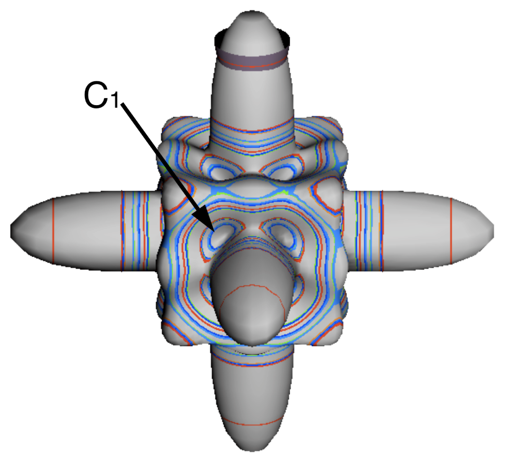
As the order of the local sub-group symmetry goes down, the degeneracy and complexity of the rotational cluster must increase. O_h⊃C_2v clusters are 12 fold degenerate and come in 4 cluster species. Matrices describing this system are larger, but O⊃C₂ will show many of the same effects. To actually resolve the doubled T₁ or T₂ triplets of O⊃C₂ requires distinguishing the u and g versions of each. The C₂ clusters are 12 fold degenerate, but they are also easily displayed.

As noted earlier, O⊃D₃⊃C₂ and O⊃D₄⊃C₂ local symmetries give identical cluster degeneracies and groupings, but with cluster splittings and structure dependent on the sub-group chain. Though it neglects inversion, Figure 27 indicates that there are several different types of O⊃C₂ (and, thus O_h⊃C_2v local sub-group symmetries). Examples given here involve the O ⊃D₄⊃C₂(i₄) sub-group chain.

Compared with O⊃C₄ and O⊃C₃, the splittings of O⊃C₂ are relatively simple to calculate since the terms in Equation (131) will be real. Creating splitting tables for C₂ is done in the same way as for Tables 11 and 12. It is shown in

Table 13. Splittings of O ⊃ C₂(i₄₎ given sub-class structure.

O ⊃ D4 ⊃C2(i4)	0°	rn120°	ρn180°	Rn90°	in180°
02
ɛ02A1	g0	4r12 + 4r34	2ρxy + ρz	4Rxy + 2Rz	4i1256 + i3 + i4
ɛ02E	g0	−2r12 − 2r34	2ρxy + ρz	−2Rxy + 2Rz	−2i1256 + i3 + i4
ɛ02T1	g0	−2r12 + 2r34	−ρz 2Rxy	−2i1256 − i3 + i4
ɛ02T2E	g0	2r12 − 2r34	−ρz	−2Rxy	2i1256 − i3 + i4
ɛ02T2A1	g0	0	−2ρxy + ρz	−2Rz	i3 + i4
12
ɛ12A2	g0	4r12 + 4r34	2ρxy + ρz	−4Rxy − 2Rz	−4i1256 − i3 − i4
ɛ12E	g0	−2r12 − 2r34	2ρxy + ρz	2Rxy − 2Rz	2i1256 − i3 − i4
ɛ12T1E	g0	2r12 − 2r34	−ρz	2Rz −	2i1256 + i3 − i4
ɛ12T1A2	g0	0	−2ρxy + ρz	−2Rz	−i3 − i4
ɛ12T2E	g0	−2r12 + 2r34	−ρz	−2Rxy	2i1256 + i3 − i4

.

8.1.1. Local Sub-Group Tunneling Matrices and Their Inverse

Table 13 can be further broken apart to demonstrate how one can create an automated process to evaluate the tunneling splittings for O⊃C₂ local-symmetry structures. What will result is a transformation between cluster-splitting energy and tunneling parameters. The inverse of this transformation is also easily defined.

Equation (131) produces Table 13, but even after combining splittings from each subclass, repetition exists. We show the two steps to convert Table 13 into the transformation matrix just described. First we assume that only n_m levels may interact with themselves, e.g., that a 1₂ cluster may not interact with a 0₂ cluster. Second we recognize that only half of the subclasses are needed to fully define the possible splittings, the others simply repeat the same information. Table 13 shows this for the 0₂ cluster. Looking at the A₁ level in the 0₂ cluster, one can see that the subclasses 1, r_n, ρ_n make a vector {1, 4, 4, 2, 1} while the R_n, i_n subclasses make a vector {4, 2, 4, 1, 1}. These vectors are reordered versions of each other. Thus only one is needed. The A₂ level in the 1₂ cluster shows the same similarity, but the R_n, i_n now contain a negative sign.

By using only the minimum number of splitting parameters and including only a single cluster gives a condensed version of Table 13 that acts as a transformation that inputs symmetry-based tunneling values and outputs energy levels. Such a table is shown in

Table 14. Matrix that converts tunneling strengths to cluster splitting energies.

02	1	r12, i1256	r34, Rxy	ρxy, Rz	ρz, i3
ɛ02A1	1	4	4	2	1
ɛ02E	1	−2	−2	2	1
ɛ02T1	1	−2	2	0	−1
ɛE,02T2	1	2	−2	0	−1
ɛA1,02T2	1	0	0	−2	1

. A simple inverse of the matrix in Table 14 will produce the transformation giving tunneling parameters for a given set of cluster energy splittings, as shown in

Table 15. Matrix that converts cluster splitting energies to tunneling strengths.

02	ɛ02A1	ɛ02E	ɛ02T1	ɛE,02T2	ɛA1,02T2
1	$\frac{1}{12}$	$\frac{1}{6}$	$\frac{1}{4}$	$\frac{1}{4}$	$\frac{1}{4}$
r12, i1256	$\frac{1}{12}$	$-\frac{1}{12}$	$-\frac{1}{8}$	$\frac{1}{8}$	0
r34, Rxy	$\frac{1}{12}$	$-\frac{1}{12}$	$\frac{1}{8}$	$-\frac{1}{8}$	0
ρxy, Rz	$\frac{1}{12}$	$\frac{1}{6}$	0	0	$-\frac{1}{4}$
ρz, i3	$\frac{1}{12}$	$\frac{1}{6}$	$-\frac{1}{4}$	$-\frac{1}{4}$	$\frac{1}{4}$

.

There are multiple ways to use Tables 14 and 15. Among the most useful is to use the columns of Table 14 as a predictor of possible splitting patterns. Using the inverse matrix to find spectroscopic tunneling parameters from cluster splittings may also become a useful and automated process.

An example demonstrates this process for a model (4, 6)-octahedral-Hecht spherical-top Hamiltonian Equation (134) with varying spectroscopic parameters. The terms T^[4] and T^[6] model rotational distortions written in an octahedral basis of fourth and sixth order respectively in J. The parameter θ is varied to explore the different relative contributions of T^[4] and T^[6] while keeping them normalized. Because T^[4] and T^[6] each have octahedral symmetry, Equation (134) represents all possible octahedral pure rotational Hamiltonians up to sixth order.

$$H=B{J}^2+\text{cos}(\theta )T^{[4]}+\text{sin}(\theta )T^{[6]}$$

(134)

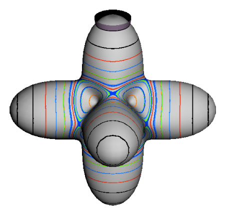
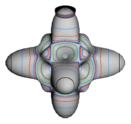
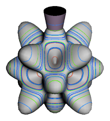
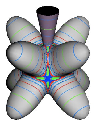
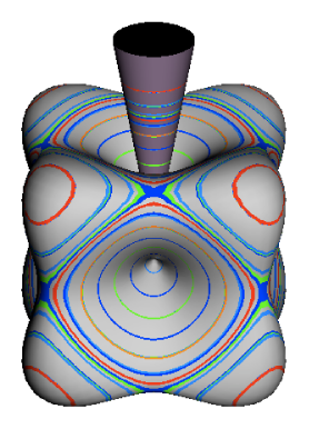
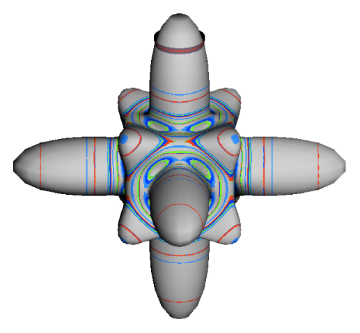
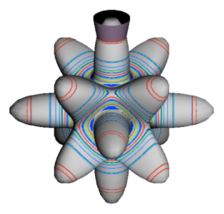
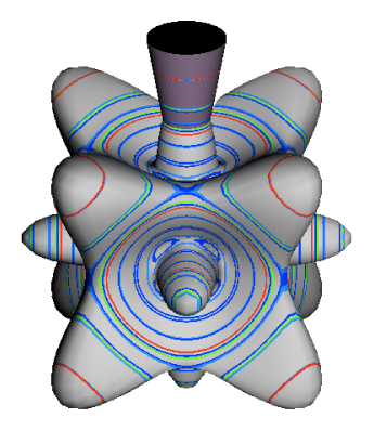
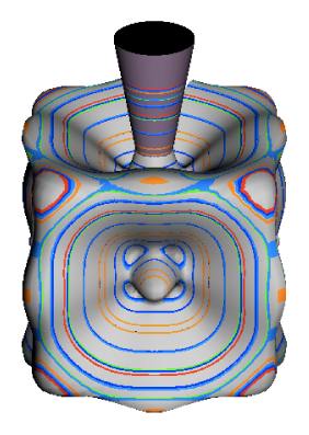
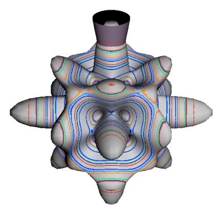
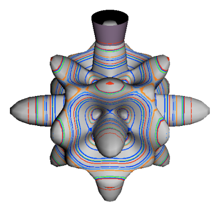
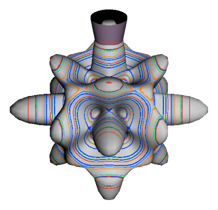
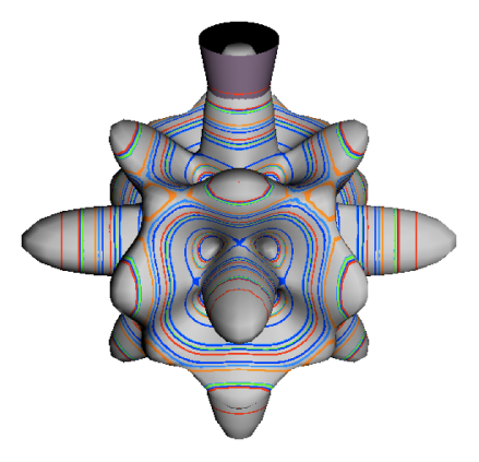
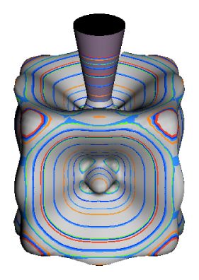
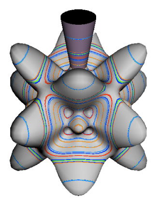
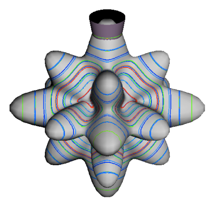
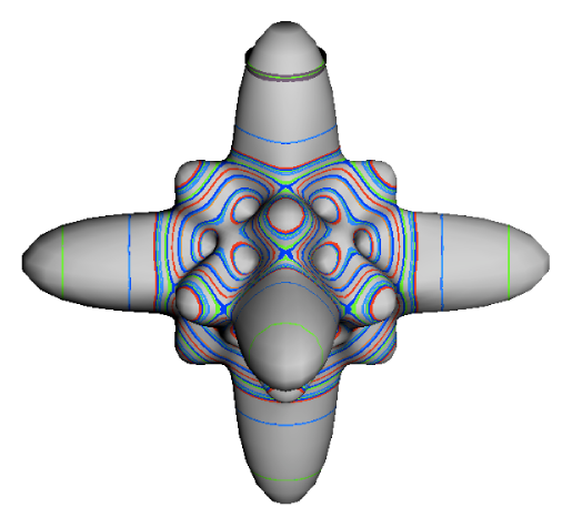
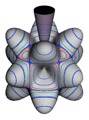
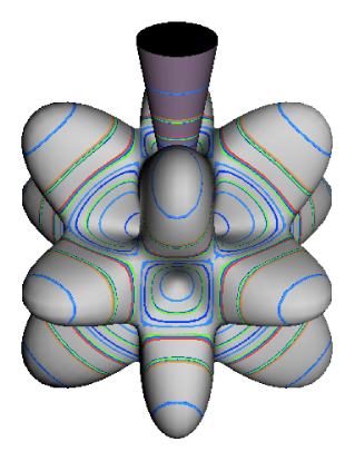
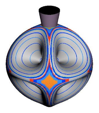
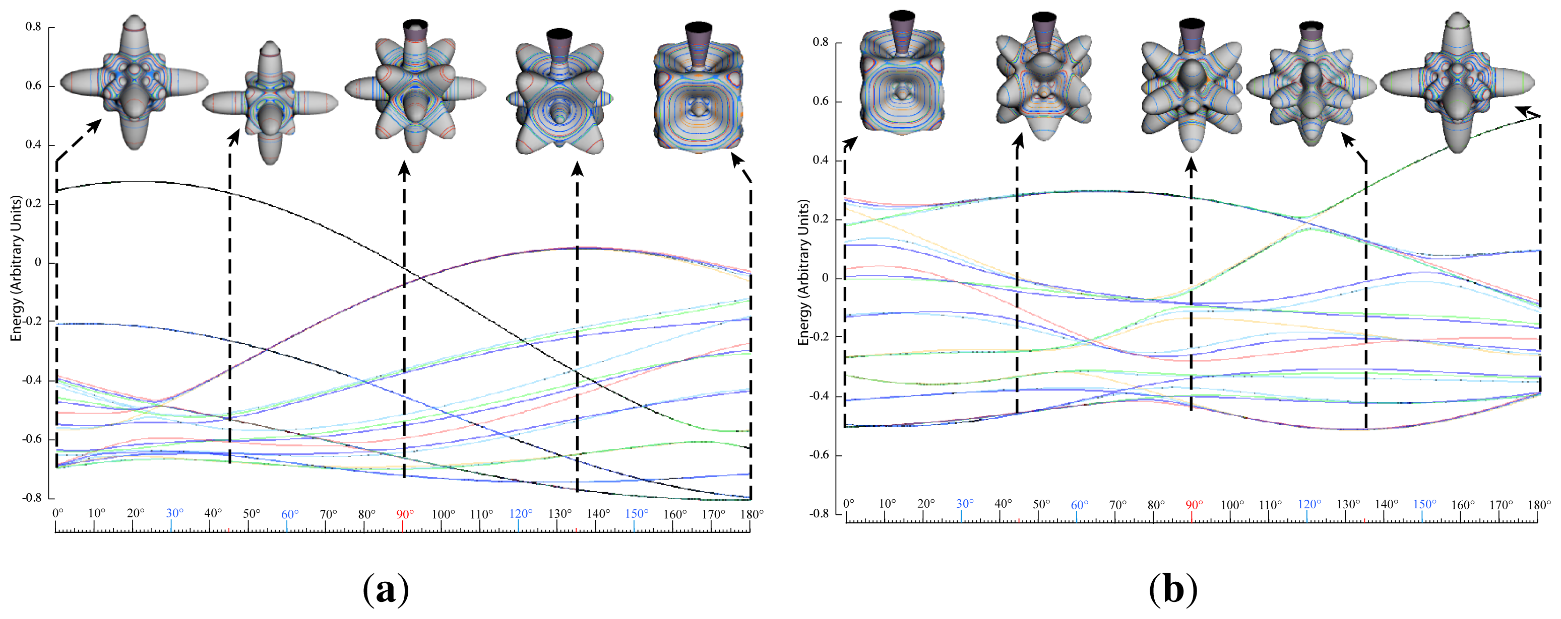
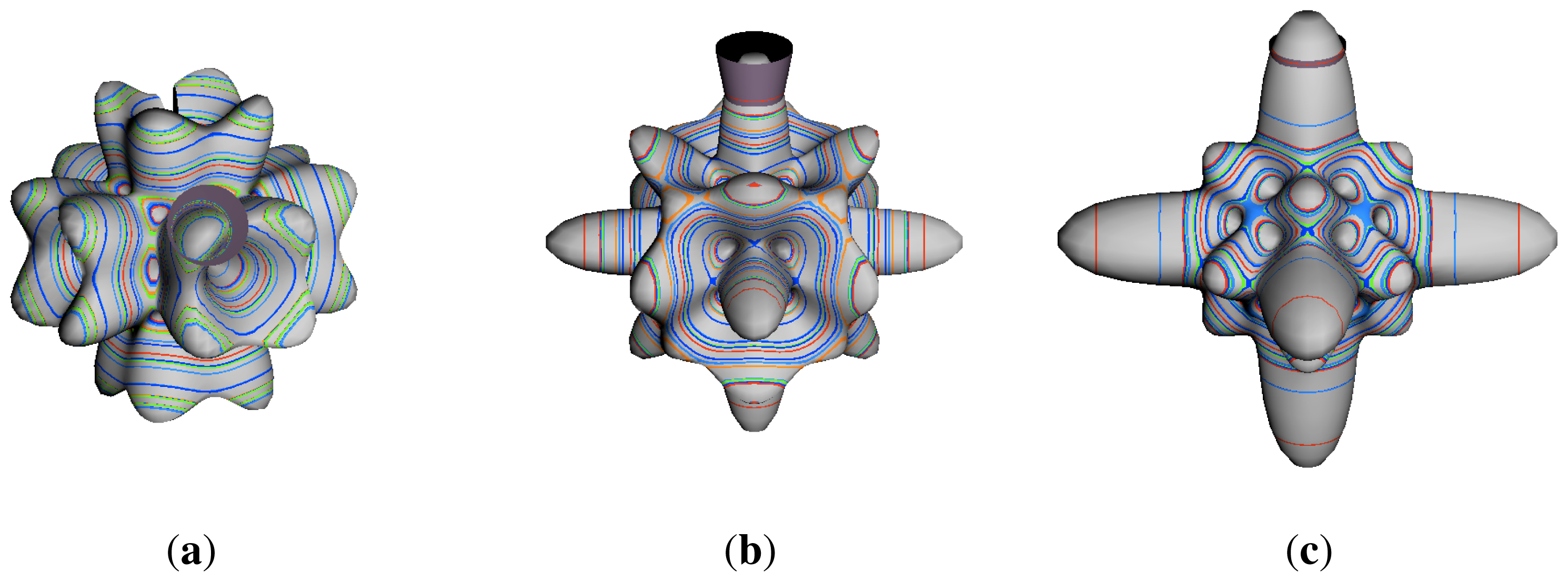
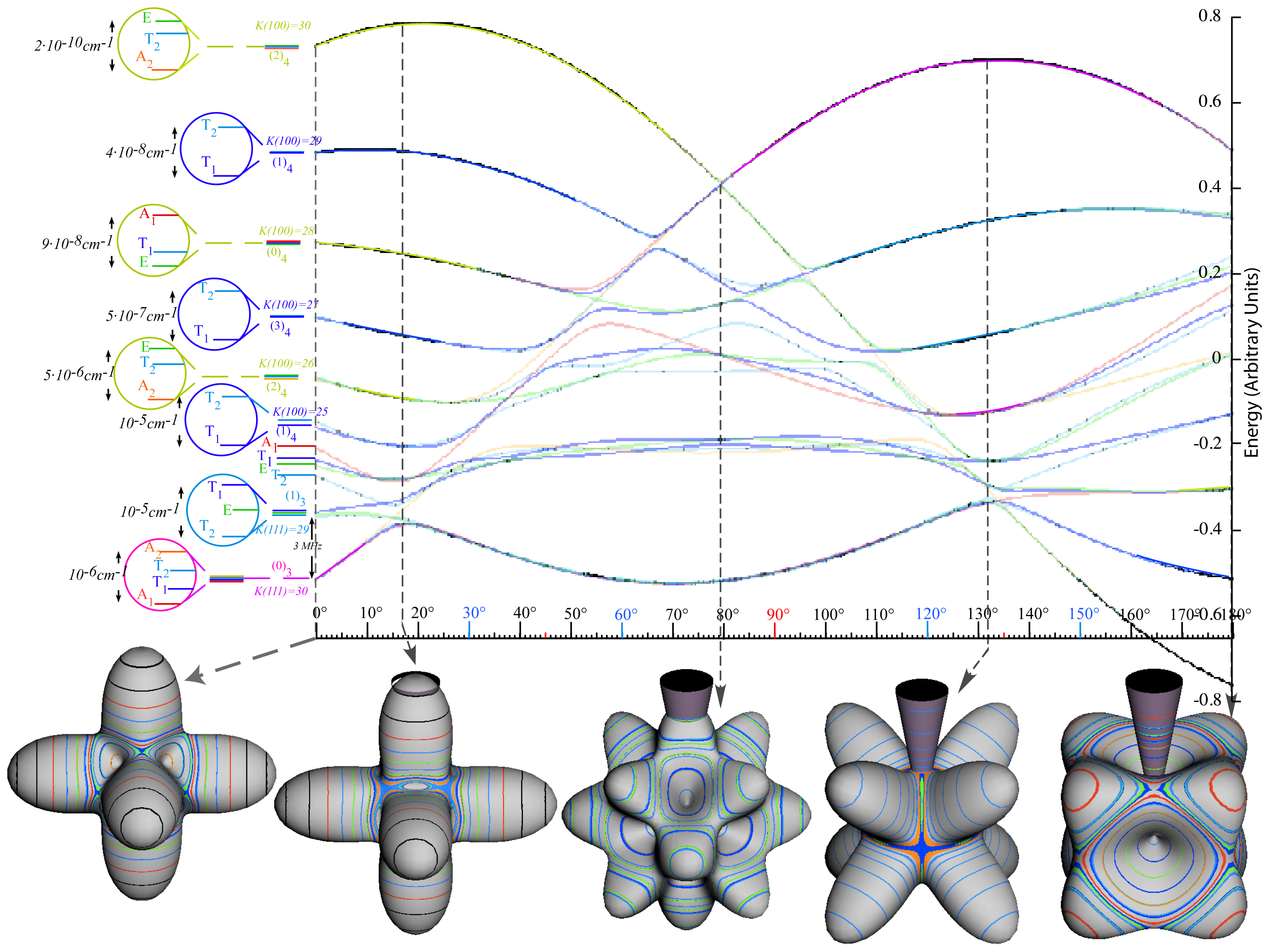
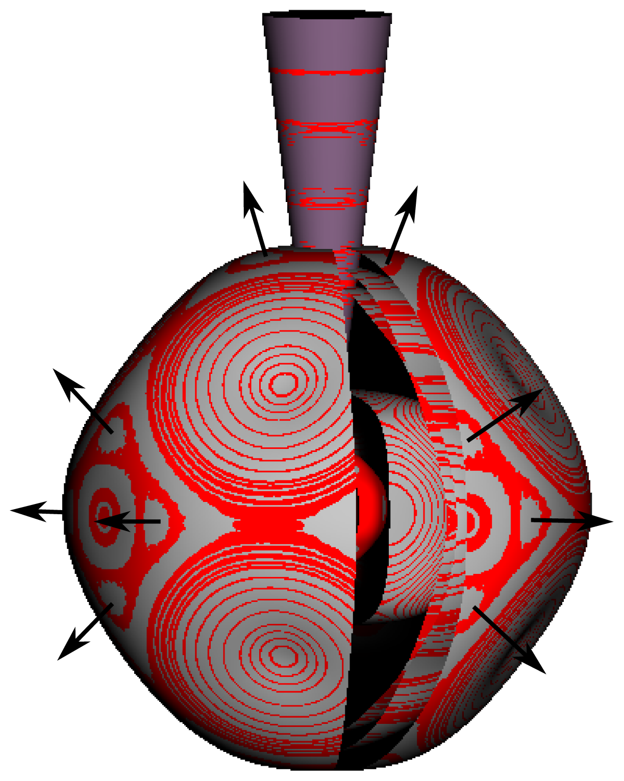
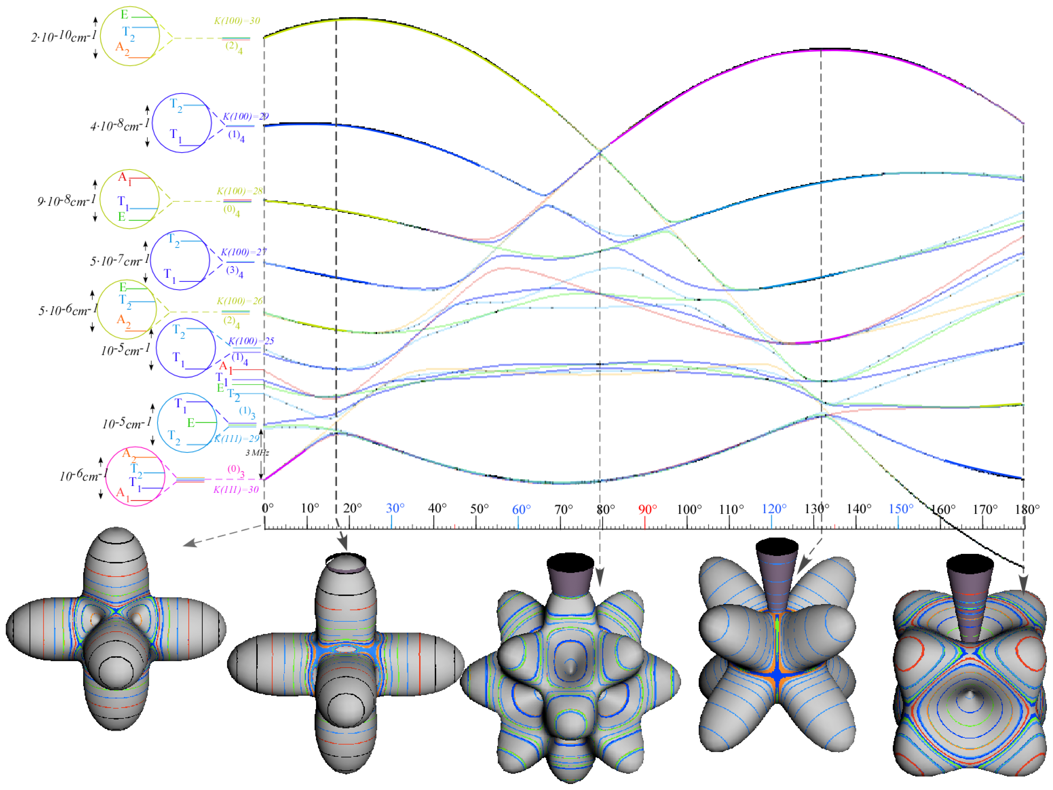
As noted in Section 3 cluster structure location and the RES shape will change significantly as the Hamiltonian parameters change in Equation (134) as Figure 29 (a copy of Figure 6) shows by plotting rotational energy levels of Equation (134) for changing θ with corresponding RES at points along the θ axis. RES plots in the figure demonstrate how the phase-space changes as θ varies.

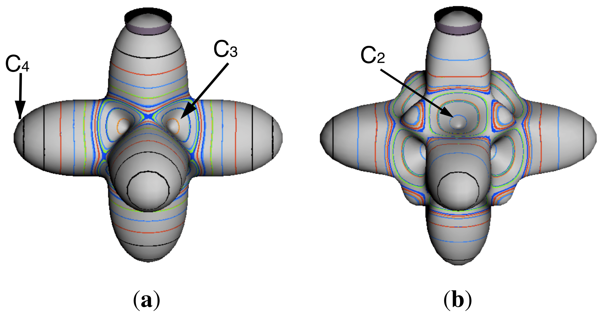
RES diagrams in Figure 29 along with the cluster degeneracy indicate where in the parameter-space C₂ clusters exist. The lowest 0₂(C₂)↑O cluster in Figure 29 for θ between 18° and 132° labels a kaleidoscope of 12 waves each with C₂ local symmetry. Its superfine levels are magnified about 100 times in the central inside plot of Figure 30 which has been adjusted to show level splittings but not whole cluster shifting. (The θ-dependent cluster center-of-energy is subtracted.) The locally antisymmetric 1₂(C₂)↑O clusters contain quite similar superfine structure but with A₂ replacing A₁ and T₁ switched with T₂.

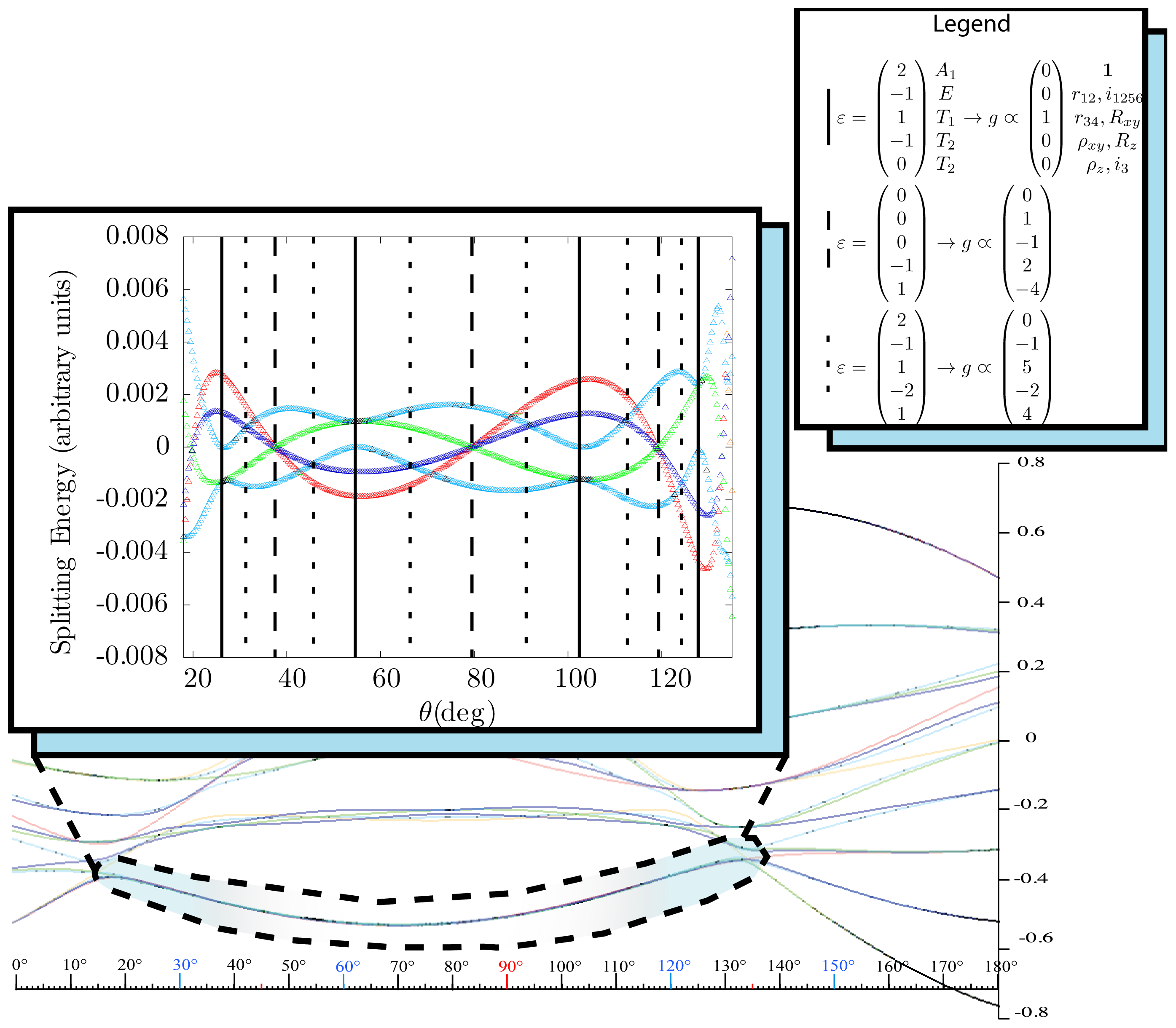
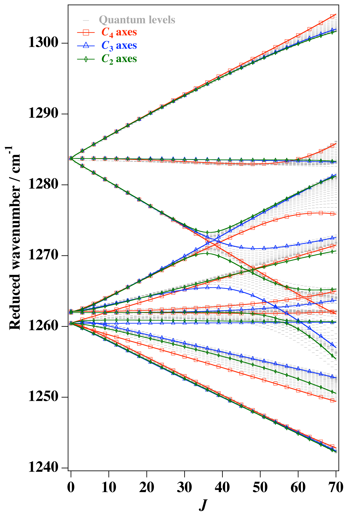
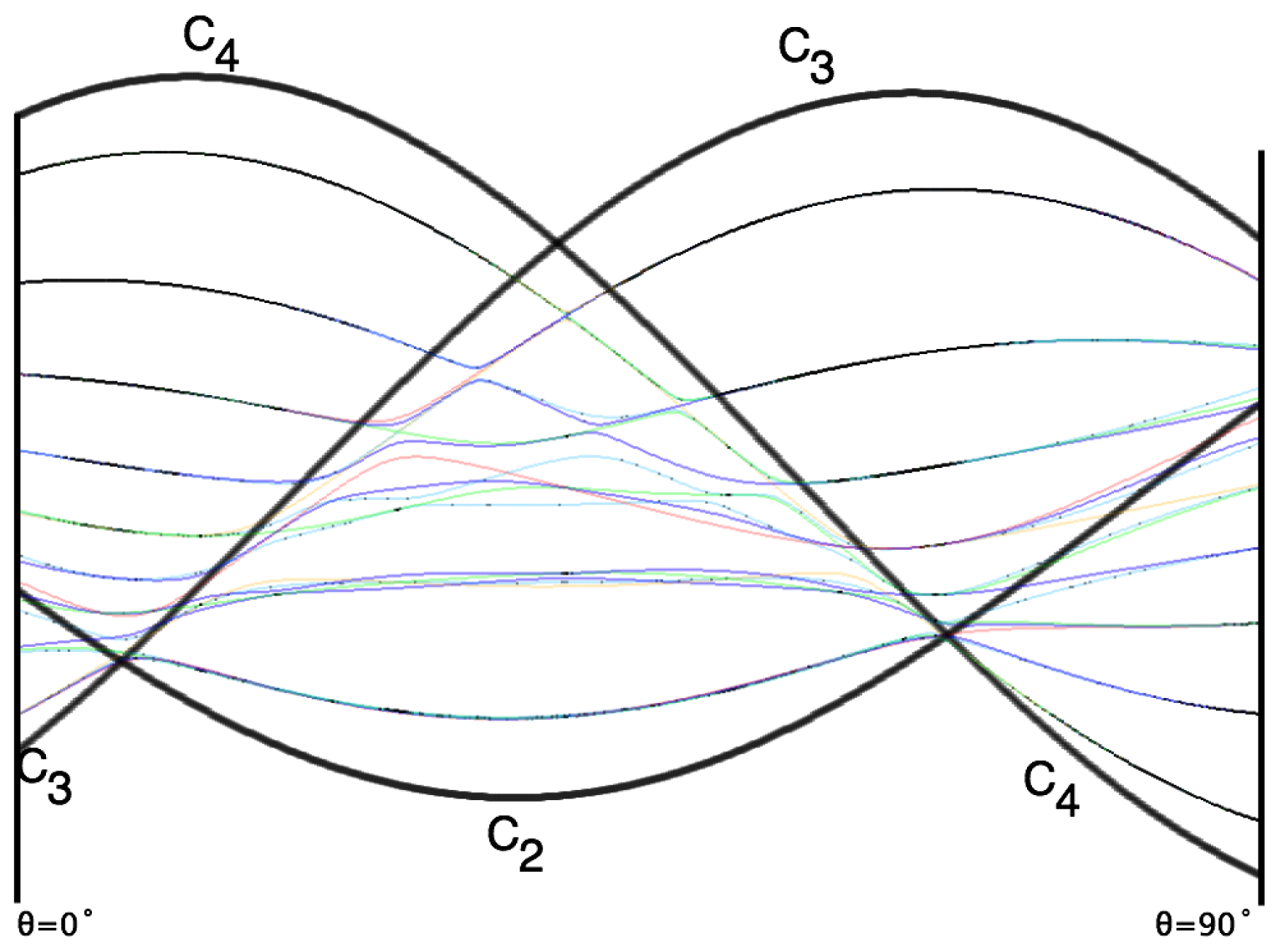
At certain θ-points in Figure 30 levels of different symmetry cross and one of three distinctive splitting patterns emerge. These points occur periodically as indicated by vertical lines that are (starting form left side) solid, dotted, dashed, dotted, solid, dotted, dashed, solid, and so forth across the plot. The three distinctive ε^α-energy level patterns for species α=(A₁, E, T₁, T₂, T₂) are given by vectors ε_dash=(0, 0, 0, 1,−1), ε_dot=(2, −1, 1, 1, −1) and ε_solid=(2, −1, 1, 0, −1), respectively. These repetitious patterns seem to persist even outside of the marked-off sections to the very ends of the C₂ cluster region at θ≃18° and θ≃132° where they grow slightly but maintain their respective superfine ratio patterns and degeneracy. The matrix in Table 15 transforms each of the three ε^α-vectors in Figure 30 into a vector of O-defined sub-class tunneling amplitudes g_r. These are evaluated for clusters at several values of parameter θ used in T^[4,6] Hamiltonian Equation (134). Proportioned values of the tunneling amplitudes g_r for the three distinctive cases are listed in the inset legend of Figure 30 based on Tables 14 and 15.

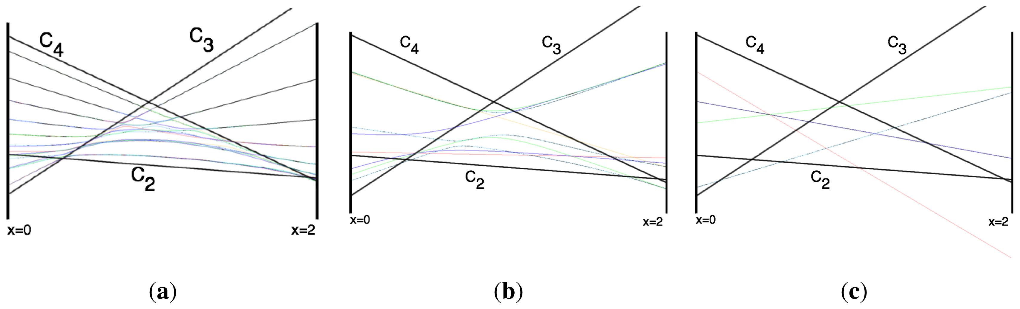
Dotted-line and solid-line curve patterns appear alternately flipped in sign. Dotted-line patterns have a crossing (T₁,T₂) pair while the solid-line patterns have a crossing (T₂,E) pair.

Solid-line patterns appear to be centered on quasi-hyperbolic avoided-level-crossing episodes involving the pair of repeated T₂ tensor species of O. The ordering (A₁, T₁, T₂, E, T₂) of solid-line superfine level patterns reflects Bohr-like orbital ordering (s, p, d, f, ..) of orbital momentum and occurs only when there is just one non-zero sub-class of tunneling parameter, namely that of sub-class (r₃₄ or equivalent R_xy) that affects tunneling between nearest-neighbor C₂ valleys.

Dashed-line pattern level curve slopes appear to alternate (+) and (−) signs and exhibit maximum separation of repeated T₂-species surrounding a degenerate (A₁, T₁, E)-sextet crossing midway in between. Such triple-point crossings are quite remarkable. They appear repeatedly in Figure 30 and persist even at low-J as seen for J=4 in Figure 8c. Higher 1₂(C₂)↑O clusters show similar triple points made of (A₂, T₂, E)-sextets.

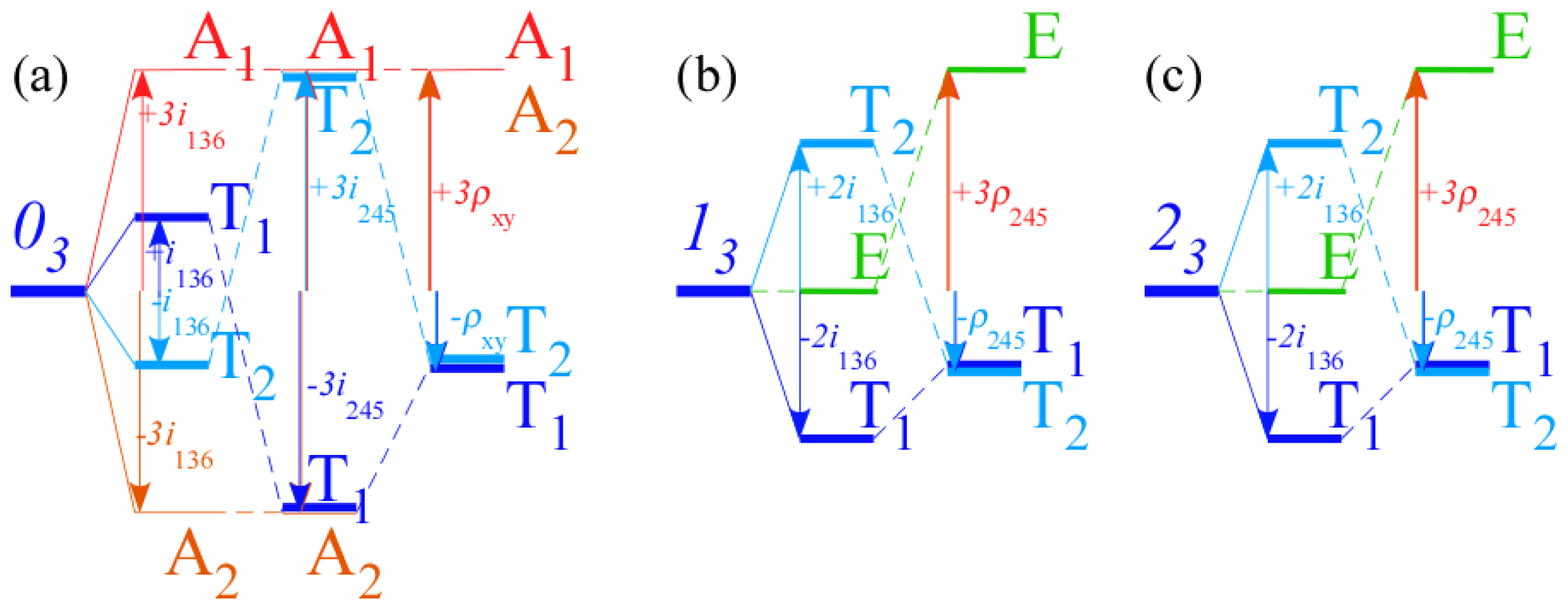
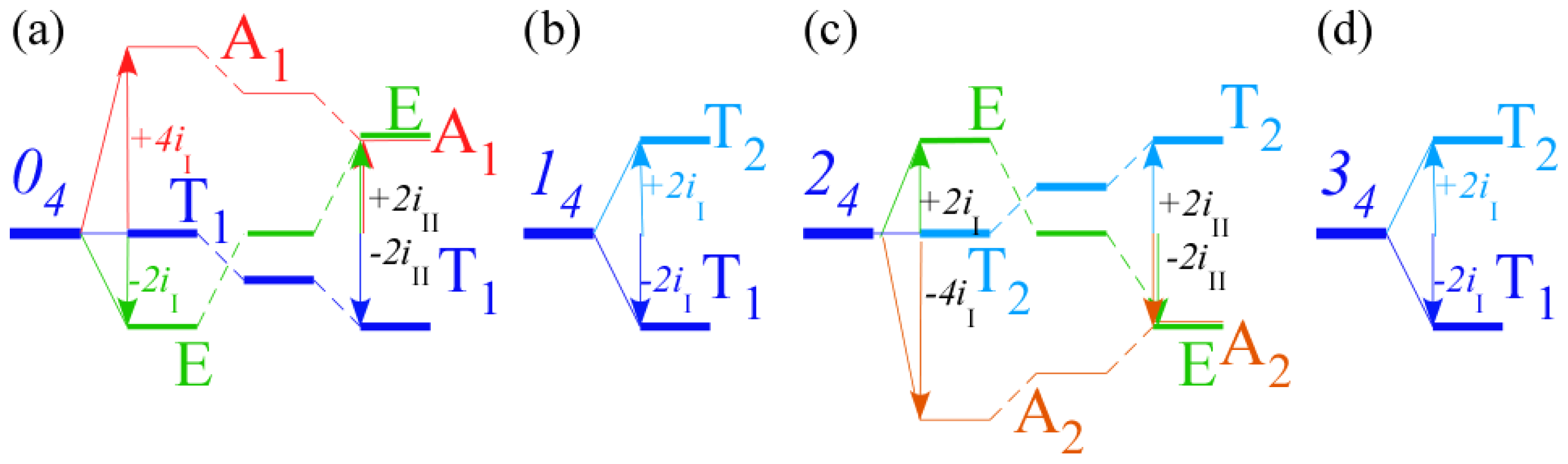
Such crossings are quite ironic if we recall that it was (A₁T₁E), (A₂T₂E), and (T₁T₂) clusters noted by Lea, Leask, and Wolf [20] and later Dorney and Watson [21] that led to a theory involving induced representations K₄(C₄)↑O including 0₄(C₄)↑O=A₁⊕T₁⊕E, 2₄(C₄)↑O=A₂⊕T₂⊕E, and ±1₄(C₄)↑O=T₁⊕T₂. (Recall C₄ columns of Equation (117) and reciprocity Equation (106)). This theory uses an inter-C₄-axial tunneling model [22,23] with a single ad.hoc. tunneling parameter that predicts a 2:1-splitting ratio for (ATE) clusters. C₄-axial tunneling cluster splitting dies exponentially as body momentum-K approaches J (Recall Figure 26) and thus C₄(ATE) levels never actually cross.

However, the C₂(ATE) levels in Figure 30 clearly do so and with quite the opposite 1:2-spltting ratio. It is ironic that the more elegant ortho-complete multi-path tunneling models, while useful in exposing these crossings, seem at a loss to explain them, particularly given that they were first noted by Lea, Leask, and Wolf so very long ago!

It would be easy to write off such (ATE) triple-crossings and particularly the (T₁T₂) or (ET) double-crossings as “accidental” degeneracy. Indeed, all but the latter occur for special values of a complete set of sub-class parameters. However, Figure 30 clearly shows that each type of crossing belong to a periodic structure that is unlikely to be just an accident.

Clearly there is still much to learn about multi-path tunneling models in general and the octahedral ones in particular. Here we can only offer a potentially elegant way to treat these kinds of high-symmetry cases.

9. Examples of Rovibronic Energy Eigenvalue Surfaces (REES) and J-Clusters

Semiclassical treatment of rovibronic or rovibrational states provides some insight into the transition between lab-coupled and body-coupled vibronic momentum that are related in Equation (8) through Equation (10b) of Sections 1 and 2. The first semiclassical analysis of fundamental coupling in high-J octahedral molecules was done for ν₂E[38] and ν₃T₁[39] bands in 1978 and for overtone ν₂ + ν₃ “hot-bands” in 1979 [40].

These methods are similar in philosophy to those described in Section 2 that approximate tensor eigenvalues with Legendre formulas and thereby construct rotational energy based on a semiclassical J-vector. However, the more general approach differs in that it builds an N-by-N matrix of such formulas that takes account of quantum rovibronic coupling between N vibronic (or vibrational) states, that is, a 2-by-2 matrix for the ν₂E system, a 3-by-3 matrix for the ν₃T₁ system, and a 5-by-5 matrix for the ν₂ + ν₃ system.

The resulting N eigenvalues provide points on N nested Rovibronic Energy Eigenvalue Surfaces (REES) for each direction of the semiclassical J-vector. Visualization of P, Q, and R state mixing in ν₃T₁ bands by 3-sheet REES was done using the high-resolution 3D-graphics at Los Alamos in 1987 and reported in 1988 [25]. Interesting features of the ν₃T₁ REES include conical intersections that occur for zero scalar Coriolis coupling. These are analogous to well known conical intersections of Jahn–Teller PES that lend insight into BOA breakdown of single adiabatic surfaces. The following contains two examples of REES models. The first is a simplified internal rotation model involving a 2-sheet REES, and the second is an excerpt of a recent study of the ν₃/2ν₄ dyad of CF₄ that involves a 9-sheet REES.

9.1. Rotor-With-Gyro Model of Internal Rotation

A first application by Ortigosa and Hougen [17] of REES to visualize molecules with internal rotation is related to a simple rotor-with-gyro model [25,41] based on the three lowest rank tensors possible, namely the scalar (rank-0), the vector (rank-1), and the tensor (rank-2). The prolate symmetric top RES in Figure 1 is an example of a scalar-tensor combination. A vector RES lacks J-inversion symmetry, that is, time reversal symmetry, so it is forbidden for normal molecules that have no intrinsic dynamic chirality such as embedded spin S. We consider how to include an S in a way that preserves overall T symmetry.

Total momentum J=R+S is the sum of rotor momentum R and gyro spin S. J is conserved in lab frame but R and S are not. If gryo is body-frame-fixed by frictionless bearing then rotor gyro-coupling does no work and is an ignorably constant H_RS. S and |J| are conserved in body frame but J and R are not.

$$H_{R+S(bod-fixed)}=A{\mathbf{R}}_x^2+B{\mathbf{R}}_y^2+C{\mathbf{R}}_z^2+H_S+H_{RS}$$

(135)

Replacing bare-rotor momentum R=J-S gives the following with a new constant spin energy H′_RS.

$$\begin{array}{c}{H}_{R,S(bod-fixed)}=A\hspace{0.17em}{({\mathbf{J}}_x-{\mathbf{S}}_x)}^2+B\hspace{0.17em}{({\mathbf{J}}_y-{\mathbf{S}}_y)}^2+C\hspace{0.17em}{({\mathbf{J}}_z-{\mathbf{S}}_z)}^2+H_{RS}\\ =A{\mathbf{J}}_x^2+B{\mathbf{J}}_y^2+C{\mathbf{J}}_z^2-2A{\mathbf{J}}_x{\mathbf{S}}_x-2B{\mathbf{J}}_y{\mathbf{S}}_y-2C{\mathbf{J}}_z{\mathbf{S}}_z+{H^{\prime }}_{RS}\end{array}$$

(136)

The simplest classical theory of the rotor-R-gyro-S momentum dynamics involves superimposed RES plots, one for +S and one for -S in Figure 31; A composite RES with T symmetry. If J and +S align (anti-align) then |R|=|J-S|, rotor energy Equation (135), and rotor-gyro relative velocity are minimized (maximized) (Thus, gyro-compass alignment with Earth rotation is seen to be relativistic quantum effect!).

A quantum theory of multiple RES involves mixing extreme cases |J ± S|. An elementary quantum gyro-spin is a two-state spin-1/2 with a 2-by-2 Hamiltonian matrix found by inserting quantum spin S=σ/2 matrices into Equation (136) to give Equation (137). Gyro-rotor dynamics involves REES obtained from eigensolutions of the following 2-by-2 matrix for each body-based J-vector Euler orientation (β, γ ).

$$\begin{array}{l}{H}_{R,S(quantized)}=A{\mathbf{J}}_x^2+B{\mathbf{J}}_y^2+C{\mathbf{J}}_z^2-A{\mathbf{J}}_x{\sigma }_x-B{\mathbf{J}}_y{\sigma }_y-C{\mathbf{J}}_z{\sigma }_z+const.\\ =\left(\begin{array}{cc}{\text{RE}}_{\text{rotor}}-JC\hspace{0.17em}\text{cos\hspace{0.17em}}\beta & -AJ\hspace{0.17em}\text{cos\hspace{0.17em}}\gamma \hspace{0.17em}\text{sin\hspace{0.17em}}\beta -iBJ\hspace{0.17em}\text{sin\hspace{0.17em}}\gamma \hspace{0.17em}\text{sin\hspace{0.17em}}\beta \\ -AJ\hspace{0.17em}\text{cos\hspace{0.17em}}\gamma \hspace{0.17em}\text{sin\hspace{0.17em}}\beta +iBJ\hspace{0.17em}\text{sin\hspace{0.17em}}\gamma \hspace{0.17em}\text{sin\hspace{0.17em}}\beta & {\text{RE}}_{\text{rotor}}+JC\hspace{0.17em}\text{cos\hspace{0.17em}}\beta \end{array}\right)\\ \text{where}:{\text{RE}}_{\text{rotor}}=J^2(A{\text{cos}}^2\gamma {\text{sin}}^2\beta +B{\text{sin}}^2\gamma {\text{sin}}^2\beta +C{\text{cos}}^2\beta )\end{array}$$

(137)

Eigensolutions of matrix form Equation (137) transform classical RES Figure 31 into quantum REES Figure 32 that has conical intersections or avoided crossing points replacing lines of classical surface intersections in the former Figure 31. Also, individual sheets of REES have J-inversion symmetry (or T symmetry) that individual RES lack. Where the RES of Figure 31 are well separated their shape is not so different from that of REES in Figure 32. Differences show up near the intersection lines where the two RES approach resonance. In this resonance region the REES is deformed extremely from rank-1 or rank-2 tensor shape of the separate RES, and there arises greater mixing of the extreme |±S| base-states.

9.2. REES of CF₄ in ν₃/2ν₄ Dyad

The first practical REES application includes 9-sheet displays of the ν₃/2ν₄ dyad of CF₄ recently shown by Boudon etal.[2]. This large scale numerical analysis may be summarized by a revealing plot of dyad eigenlevels as a function of J = 0 to 70 in Figure 33. This includes colored lines representing the REES values for J located on C₄ axes (shaded red), C₃ axes (shaded blue), or C₂ axes (shaded green).

Each of the symmetry axes may take turns as central loci for clusters of their type of local symmetry C₂, C₃, or C₄, or else, they may sit on a REES separatrix or saddle point between two or more different types of clusters. A third option involves C₁ clusters that have no rotation axis point but are likely to belong to vertical xyz-plane reflection symmetry C_v = [1, ρ_z] or diagonal-plane reflection symmetry C_d = [1, i₃]. These label clusters of 24 levels associated with 24 equivalent REES hills or valleys.

A final option involves true-C₁ clusters with no local symmetry whatsoever and 48 REES hills or valleys. So far this extreme type has not been identified, but one may speculate that it may actually become most common at extremely high J.

A common ordering noted before on the left hand side of Figure 29 (pure T^[4]) and in Figure 26 (16μ region of SF₆) is (C₃-valley→C₂-saddle→C₄-hill). It is present in the lowest REES band of Figure 33. An inverted version of the common ordering appears clearly in the 2^nd band whose REES is cubic in Figure 34.

A cutaway view at J = 57 of the first five REES sheets shows glimpses of the first two REES deep inside of Figure 34. The second sheet has cubic topography similar to the inverted T^[4] RES on the right hand side of Figure 29 (pure (−)T^[4]). However, the first and lowest REES for J = 57 is practically spherical with all 2J + 1=115 levels and clusters crushed in Figure 33 into near degeneracy!

After the first two REES sheets the cluster topography become more complicated with multiple conical intersections and avoided crossing points.

On the 5^th sheet of the (J = 57)ν₃/2ν₄ REES are found examples of C₁-local symmetry valleys as shown in Figure 34. (The upper four sheets are made invisible.) Each C₁ loop occupies an area that is comparable to the minimum uncertainty (J = K)-cone shown on vertical C₄ axis of the figure and a nascent 24-level cluster of type 1₂(C₂)↑O should be present in the level spectrum.

The symmetry details in this rovibrational spectra and the potential richness of quantum dynamics it represents should be quite evident from the few examples glimpsed here. We seem to be just scratching the surface of quantum systems of a great but potentially comprehensible complexity.

10. Summary and Conclusions

Semiclassical methods for visualizing and analyzing rovibrational dynamics of symmetric polyatomic molecules have been reviewed. This includes improved understanding of RES and REES phase spaces and development of more powerful symmetry methods to calculate tunneling dynamics of symmetric molecules that are highly resonant. A group-table-matrix analysis of intrinsic vs. extrinsic symmetry duality (The “Mock-Mach-Principles” Equation (95) and Equation (94) of wave relativity.) leads to generalizing character relations between group classes and irreducible representation into sub-character relations between sub-classes and induced representations Equation (131) and (132). These provide ortho-complete parameter relations (Tables 11–15) for complex tunneling path lattices that determine molecular fine, superfine, and hyperfine spectra. The methods may be extensible to fluxional atomic and molecular systems.