Thermodynamic, Structural and Transport Properties of Lennard-Jones Liquid Systems. A Molecular Dynamics Simulations of Liquid Helium, Neon, Methane and Nitrogen

Abstract

Molecular dynamics calculations are carried out in order to find the properties of Lennard Jones liquids in different state points of their phase diagram. The spherical shape and the stability of the helium, neon, methane and nitrogen make the liquids easily accessible to numerical simulation. Thermodynamic, structural, and transport properties are studied and compared with both experimental data and recent theoretical investigations. In the present work, up to 22 state points are covered, some of which are near or at the triple point. It will be shown that the classical approach leads to data that are in very good agreement with experiments and other types of calculations. At high temperatures and low densities, we observe a decrease in the uncertainties in the stress autocorrelation function by increasing the number of iterations.

Introduction

The prediction of thermodynamic properties of liquids and mixtures is still an issue of interest in simulation. The literature shows that these systems are widely investigated in both experimental and theoretical ways [1,2,3,4,5]. X-rays scattering of liquid methane near the triple point (90.7 K°) [6,7,8,9,10], and liquid nitrogen [11] were studied. Theoretically new simulations with path-integral formalism have been conducted to obtain thermodynamic properties, and the quantum radial functions involving Feynmann-Hibbs potentials were used for liquid helium[12]. The equilibrium and non-equilibrium properties of methane were studied with Monte-Carlo (MC) [2,3,13] and Molecular Dynamics (MD) [14,15] simulations. Moreover, various potential models have been proposed for reproducing data for these liquids[16,17,18,19,20,3,21,22]. For liquid neon, several simulations involving different approaches were performed: Path-Integral Monte-Carlo (PIMC) [23,24], Path-Integral Brownian Dynamics (PIBD) [24], Monte-Carlo simulations using two effective pair potentials arising from Path-Integral formalism, the quadratic Feynmann-Hibbs(QFH), the Gaussian Feynmann-Hibbs (GFH) and the perturbation theory [25]. These works focused mainly on the radial distribution function for a complete structural investigation of these liquids, and recent calculations [3,21,22], taking into account quantum effects, cover only some state points of the phase diagram and offer no way to approach the transport properties accurately. In this work, we propose a complete study over 22 state points and most structural, thermodynamic and transport properties are studied. Statistical accuracy of calculated data are carried out and compared to available data, either experimental or theoretical.

Numerical Model

Molecular Dynamic calculations were performed on a sample of size N = 864 molecules of masse m. The molecules interact by Lennard-Jones pair potential

$$U^{LJ}(r)=4\epsilon \left({\left(\frac{\sigma }{r}\right)}^{12}-{\left(\frac{\sigma }{r}\right)}^6\right) ,$$

(1)

specified by the parameters ε and σ. The units of energy, length, and mass were chosen to be, respectively ε, σ, and m. The corresponding microscopic time scale is specified by the parameters ε and σ. The units of energy, length, and mass were chosen to be, respectively ε, σ, and m. The corresponding microscopic time scale is $\tau ={\left(\frac{m{\sigma }^2}{\epsilon }\right)}^{1/2}$. The state of our system is specified through the reduced number density and temperature ρ^* =ρ σ³ and T^* = k_B T/ε. The thermodynamic state points sp(ρ,T) of the systems of interests methane, helium, nitrogen and neon are summarized in Table 1. The two sp of liquid helium (Hesp1, Hesp7) were chosen for comparison with Sesé’s work[12]. For liquid methane, the sp (Msp1, Msp4, Msp8) were taken from Sesé’s work [3]. The other state points were taken to complete our data production for methane in the liquid state. The first sp Nesp1 ( the triple point ) and the corresponding (ρ,T) data of liquid neon were taken from Singer and al studies [24]. The last three sp ( Nesp2, Nesp3, Nesp4) belonging to the isotherm 35.05 K° and their data were taken close to those of Raveché and al [26]. These four sp were also studied by Sesé [27]. Finally, the sp for liquid nitrogen (N2sp1, N2sp2) were taken from Narten and al [11].

The equations of motion were solved using the leap-Frog integration scheme with a constant time step algorithm (Δt = 0.5×10^-14s) and wherein the temperature T was kept constant by the constraint method [28,29]. Periodic boundary conditions around the central cubic box and the minimum image truncation were included in the calculations; long-range corrections were also applied. The starting

Table 1. Type of fluids with the value of the Lennard-Jones parameters, and thermodynamic state points investigated in this work. Densities and temperatures are in real and reduced units.

State Point	System	T (K)	T*	ρ (g/cm3)	ρ*	σ/A°	ε/kB	m/amu
Hesp1[10]	He(l)4	2.044	0.2	0.1452	0.3650	2.5565[1]	10.22[1]	4.0026
Hesp2	He(l)4	3	0.2937	0.1414	0.3554
Hesp3	He(l)4	4	0.3914	0.1289	0.3240
Hesp4	He(l)4	5	0.4895	0.1014	0.2549
Hesp5	He(l)4	5.1	0.5	0.0947	0.2380
Hesp6	He(l)4	5.1	0.5	0.0483	0.1216
Hesp7[10]	He(l)4	5.1	0.5	0.1452	0.3650
Msp1[3]	CH4(l)	91.0	0.6103	0.4495	0.8851	3.743[2]	149.1[2]	16.04303
Msp2	CH4(l)	99.8	0.6692	0.4407	0.8678
Msp3	CH4(l)	105.4	0.7069	0.4331	0.8528
Msp4[3]	CH4(l)	108.0	0.7243	0.4263	0.8394
Msp5	CH4(l)	110.9	0.7437	0.4253	0.8375
Msp6	CH4(l)	116.5	0.7813	0.4173	0.8217
Msp7	CH4(l)	122.1	0.8189	0.4091	0.8056
Msp8[3]	CH4(I)	125.0	0.8384	0.4005	0.7887
Msp9	CH4(I)	127.6	0.8558	0.4006	0.7888
Nesp1[22]	Ne(l)	24.50	0.6653	1.249	0.8084	2.789[22]	36.83[22]	20.183
Nesp2[24]	Ne(l)	35.05	0.9517	1.116	0.7528
Nesp3[24]	Ne(l)	35.05	0.9517	1.112	0.7246
Nesp4[24]	Ne(l)	35.05	0.9517	1.062	0.6877
N2sp1[9]	N2(l)	66.0	0.6496	0.8498	0.8783	3.636[9]	101.6[9]	28.0134
N2sp2	N2(l)	80.0	0.7874	0.6205	0.6414

Table 1. Type of fluids with the value of the Lennard-Jones parameters, and thermodynamic state points investigated in this work. Densities and temperatures are in real and reduced units.

State Point	System	T (K)	T*	ρ (g/cm3)	ρ*	σ/A°	ε/kB	m/amu
Hesp1[10]	He(l)4	2.044	0.2	0.1452	0.3650	2.5565[1]	10.22[1]	4.0026
Hesp2	He(l)4	3	0.2937	0.1414	0.3554
Hesp3	He(l)4	4	0.3914	0.1289	0.3240
Hesp4	He(l)4	5	0.4895	0.1014	0.2549
Hesp5	He(l)4	5.1	0.5	0.0947	0.2380
Hesp6	He(l)4	5.1	0.5	0.0483	0.1216
Hesp7[10]	He(l)4	5.1	0.5	0.1452	0.3650
Msp1[3]	CH4(l)	91.0	0.6103	0.4495	0.8851	3.743[2]	149.1[2]	16.04303
Msp2	CH4(l)	99.8	0.6692	0.4407	0.8678
Msp3	CH4(l)	105.4	0.7069	0.4331	0.8528
Msp4[3]	CH4(l)	108.0	0.7243	0.4263	0.8394
Msp5	CH4(l)	110.9	0.7437	0.4253	0.8375
Msp6	CH4(l)	116.5	0.7813	0.4173	0.8217
Msp7	CH4(l)	122.1	0.8189	0.4091	0.8056
Msp8[3]	CH4(I)	125.0	0.8384	0.4005	0.7887
Msp9	CH4(I)	127.6	0.8558	0.4006	0.7888
Nesp1[22]	Ne(l)	24.50	0.6653	1.249	0.8084	2.789[22]	36.83[22]	20.183
Nesp2[24]	Ne(l)	35.05	0.9517	1.116	0.7528
Nesp3[24]	Ne(l)	35.05	0.9517	1.112	0.7246
Nesp4[24]	Ne(l)	35.05	0.9517	1.062	0.6877
N2sp1[9]	N2(l)	66.0	0.6496	0.8498	0.8783	3.636[9]	101.6[9]	28.0134
N2sp2	N2(l)	80.0	0.7874	0.6205	0.6414

configuration is face-centred cubic (FCC) lattice for molecule positions. Initial molecular velocities were obtained from the Maxwell-Boltzmann distribution. The equilibration period is extended up to duration of 20 ps. The production phase of data, starting after the equilibration, goes on for 100 ps in order to increase the accuracy of the stress autocorrelation function. The velocity autocorrelation function (VAF) is a single-particle function and all particles are indistinguishable in a pure substance, the statistical precision of a calculation for Ψ(t) can be improved by averaging over all N particules in a system[30]. The equation is

$$\psi (t)=\frac{1}{N}\langle {\displaystyle \sum _i^N{\nu }_i}\left(t\right).{\nu }_i(0)\rangle ,$$

(2)

where ν_i(t) are the velocitys of atoms at time t. The self-diffusion coefficient D of a particule is evaluated by the Einstein and Green-Kubo formulas [30]:

$$D=\frac{1}{6N}\underset{t\to \infty }{\lim }\frac{d}{dt}\langle {\displaystyle \sum _i^N{\left[r_i(t)-r_i(0)\right]}^2}\rangle ,$$

(3)

where r_i(t) are the positions of the particles at time t. D is proportional to the slope of the mean-square displacement (MSD) at long times. The shear viscosity coefficient η can be evaluated from both Green-Kubo and generalized formulas [31]. For soft-body potentials, most simulators have used the Green-Kubo equation [30], which is an integral over the stress autocorrelation function,

$${\eta }_{xy}=\frac{1}{V{k}_{B}T}{\displaystyle {\int }_0^{\infty }\langle J_{xy}(t).J_{xy}(0)\rangle dt} .$$

(4)

The component of the microscopic stress tensor is given by

$$J_{xy}(t)={\displaystyle \sum _{i=1}^N\left(m{v}_i^x{v}_i^y-\frac{1}{2}{\displaystyle \sum _{i\ne j}\frac{r_{ij}^x{r}_{ij}^y}{r_{ij}}\frac{\partial U_{ij}}{\partial r_{ij}}}\right)} .$$

(5)

The stress autocorrelation function necessarily involves the entire system; consequently, we cannot improve the statistical precision of results for viscosity by averaging over the N particles in the system. However, for stationary, homogeneous, uniform fluids, the statistical precision can be improved somewhat by averaging over all three terms that result from the stress tensor,

$$\eta =\frac{1}{3}\left({\eta }_{xy}+{\eta }_{yz}+{\eta }_{zx}\right).$$

(6)

Results and Discussions

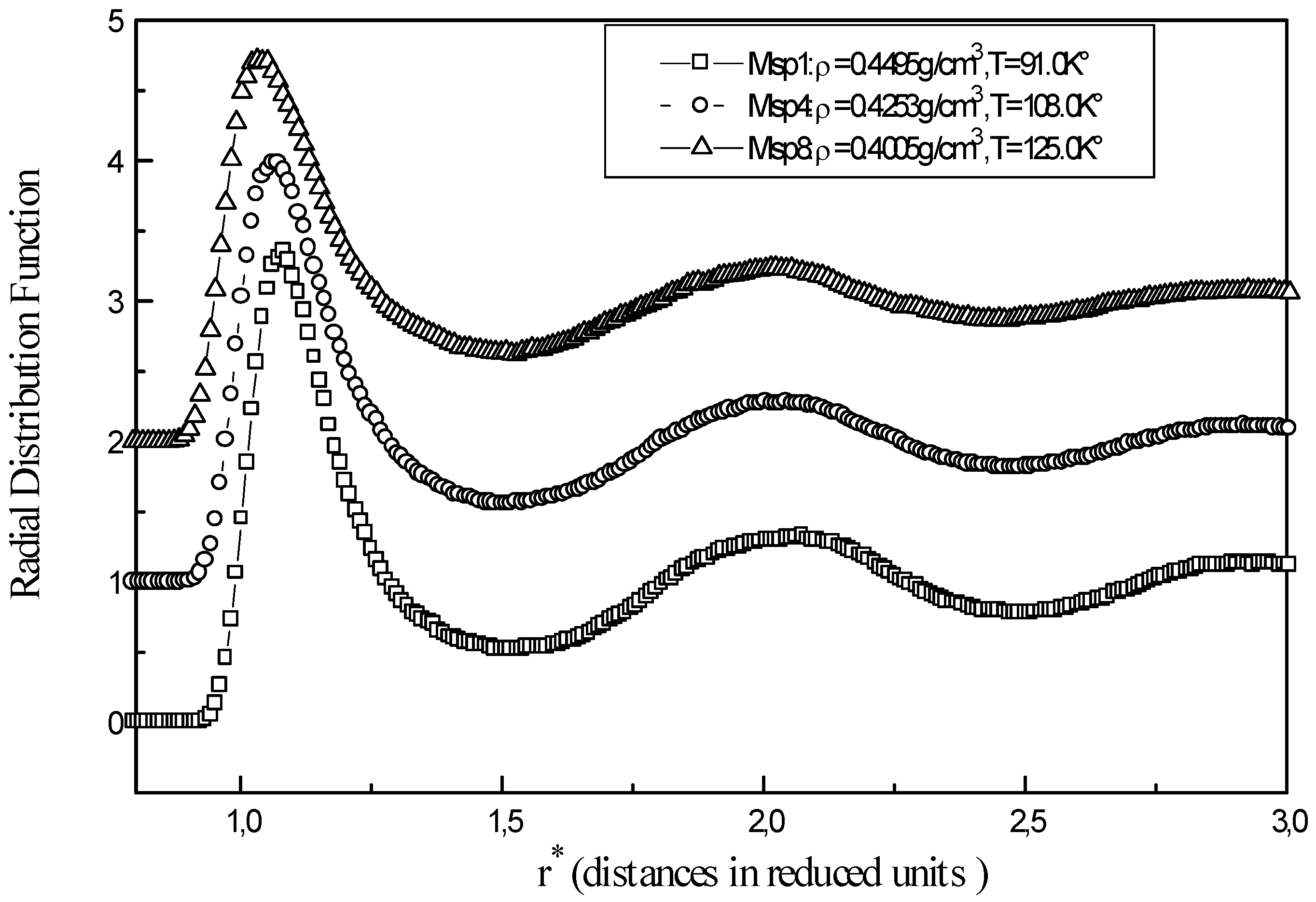
The figures presented in what follows are only illustrative of the data that can be obtained through our calculations (r* = r/σ and t* = t/τ denote distances and time in reduced units). Figure 1 shows the relevant structural information for three representative points Msp1, Msp6 and Msp9 of liquid methane. The function g(r) becomes firstly zero at short distances, where repulsive forces prevent overlapping of molecules. When r is close to the collision diameter $\underset{¨}{\mathrm{\sigma }}$g(r) increases rapidly to a maximum r = r_m corresponding to the first peak. As r increases gradually, g(r) decreases showing that influence of the central molecule is disappearing and there is no order at long distances. The average number of neighbours for a methane molecule is obtained from

$$n(R)=4\pi \rho {\displaystyle \underset{0}{\overset{R}{\int }}{r}^{2}g(r)dr,}$$

(7)

where the integration limit R is taken as the position of the successive minima in g(r).

For the Msp1, the number of nearest neighbours is 11,05 molecules and the total number of methane molecules up to the second layer is 34,36. At a temperature of T=92K°, the g(r) from X-ray diffraction gives a number of nearest neighbours ≈12 molecules and the number of neighbours in the second layer of about ≈ 55 [6]. Sesé[3] has obtained similar radial distribution function to those of the present calculations (Fig. 1) for points Msp1, Msp4, Msp8 with peak positions at different maximum Rmax1= 4.05Å and Rmax2 = 7.75 Å and minimum R min1 = 5.75-5.85 Å.

Figure 1. Radial distribution function of liquid methane at different points (Msp1, Msp2, Msp8 )

Figure 1. Radial distribution function of liquid methane at different points (Msp1, Msp2, Msp8 )

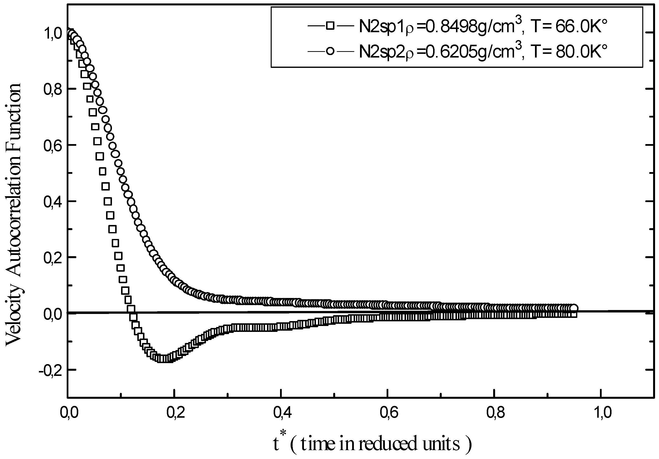
The velocity autocorrelation function ψ(t) illustrated in Figure 2 explains liquid nitrogen mobility. The results show different behaviour for the function ψ(t) for N2sp1 and N2sp2. The increase in temperature put a pressure upon the trend of the velocity autocorrelation function. At higher densities, molecules are formally packed up, as a consequence collisions and bounced motions are more likely to occur than dispersing collisions, this causes instability at point N2sp1 and ψ(t) goes through a minimum. At low density, collisions scatter molecules without changing their trajectories therefore, ψ(t) become positive ( N2sp2).

Figure 2. Velocity autocorrelation function of liquid nitrogen at different points (N2sp1, N2sp2).

Figure 2. Velocity autocorrelation function of liquid nitrogen at different points (N2sp1, N2sp2).

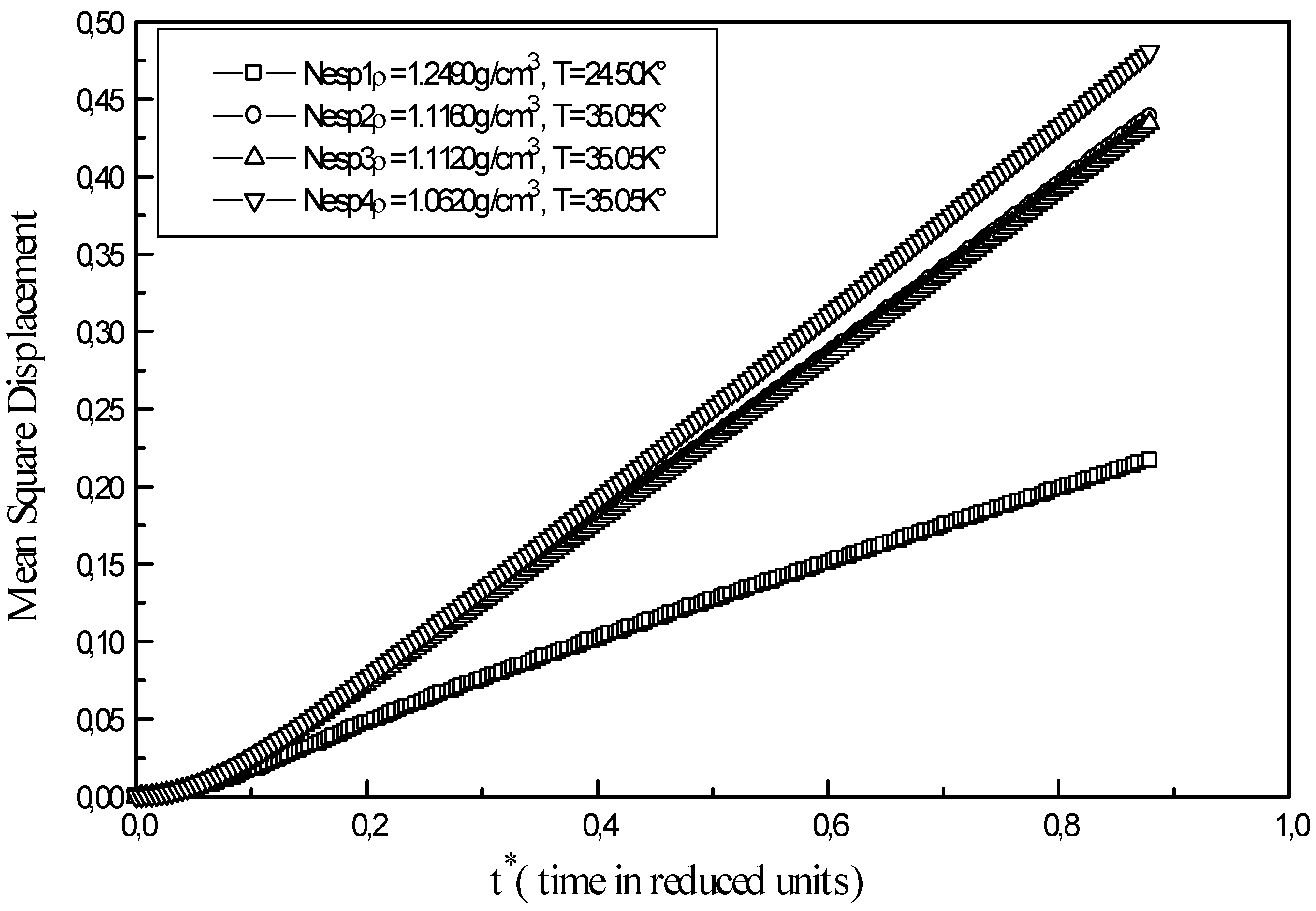
Figure 3. Mean square displacement of liquid neon at different points ( Nesp1, Nesp2, Nesp3, Nesp4 )

Figure 3. Mean square displacement of liquid neon at different points ( Nesp1, Nesp2, Nesp3, Nesp4 )

The mean square displacement of atom of liquid neon at different state points is reported in Figure 3.

At low densities the curve shows two steps. In the first stage 0.0 < t* < 0.1 the system behaves like a crystal state rather then a liquid state. Arrangement of atoms at short distances shows a certain degree of dependence, which makes one think of permanent correlations existing in the solid state. In the second stage, a change in the slope is observed with a linearly rising mean square displacement; in this case, atoms possess enough kinetic energy. Points along the 35.05 K° isotherm of liquid neon ( Nesp2, Nesp3, Nesp4) present the same profile. As time increases, an important gap appears between curves of the isotherm and the curve of triple point ( Nesp1). Equilibrium is reached faster at low densities and high temperatures and the overall runtime of a simulation is more important for the calculation of transport properties at high densities.

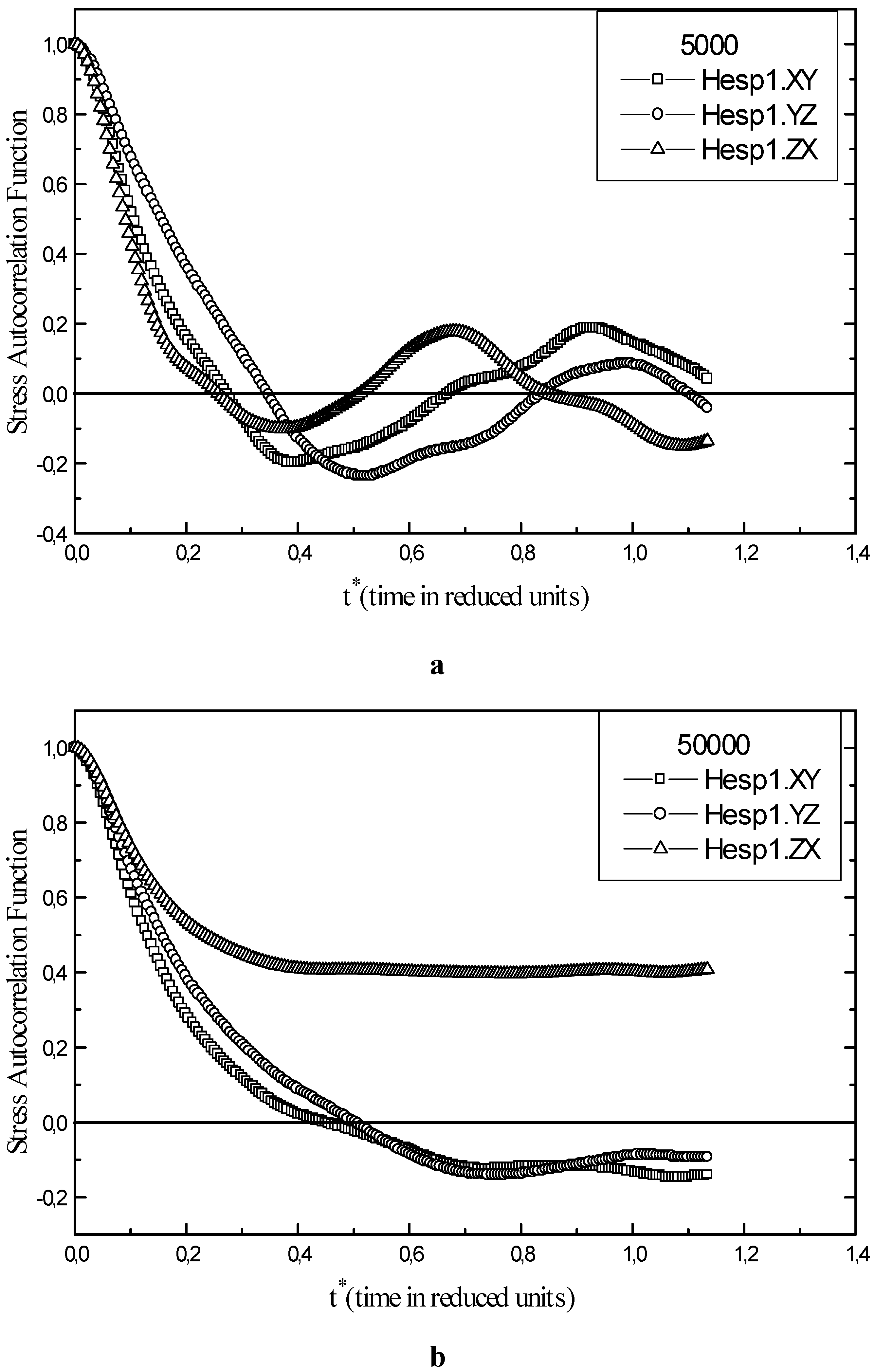
The stress autocorrelation function calculated for each points of the phase diagram and for every fluid allow us to work out the shear viscosity η. For the sp Hesp1 of liquid helium, the stress autocorrelation function is illustrated in Fig. 4a according to the three orientations. An increase of the number of iteration by a factor of 10 (from 5000 to 50000) decreases the uncertainties on η(t) as shown in Fig. 4b. The uncertainty vary about between 0.2 and – 0.2 through the time (for example, for t*=0.75 it is in order of 0.2 ). At high densities and low temperatures, we observe an increase in the calculated uncertainties. On the other hand, by increasing the calculation time, a good statistical precision of the stress autocorrelation function is achieved .

Figure 4. Stress autocorrelation function of liquid helium for state point Hesp1. a) An overall runtime of 5000 steps. b) An overall runtime of 50000 steps.

Figure 4. Stress autocorrelation function of liquid helium for state point Hesp1. a) An overall runtime of 5000 steps. b) An overall runtime of 50000 steps.

Table 2 shows calculated averages of different thermodynamic properties for every system of interest in different state points of their phase diagram. Different observations can be made. The fluctuations of properties such as the energy of configuration U, the total energy E and the enthalpy H for all states points do not show any changes. Fluid helium shows an unstable character because of the neglect of the quantum effects in this simplified model. We may notice very large fluctuations for liquid methane at points Msp1and Msp2, this is probably because these sp are close to the the triple point ( T=90.7K°). When moving over pressure data column of Table 2, an increase of pressure is

Table 2. Thermodynamic properties calculated in reduced units for different systems. Pressure P^*=P ε σ^-3 Total Energy E^*=E/Nε, Configurational Energy U^*=U/Nε, Enthalpy H^*=H/Nε, Self-Diffusion Coefficient ${\mathrm{D}}^{*} = \mathrm{D} \sqrt{\raisebox{1ex}{$m$}\!\left/ \!\raisebox{-1ex}{$z$}\right.} / \mathrm{\sigma }$, Shear Viscosity η^* = η σ³ / ε τ.

State point	System	T*	ρ*	P*	E*	U*	H*	D*	η*
Hsp1	He(l)4	0.2	0.3650	-0.107±0.016	-5.845±0.012	-6.146±0.014	-6.140±0.047	0.0034±0.0004	1.75±0.0001
Hsp2	He(l)4	0.2937	0.3554	-0.097±0.019	-5.412±0.101	-5.853±0.099	-5.685±0.094	0.0095±0.0005	1.87±0.0001
Hsp3	He(l)4	0.3914	0.3240	-0.074±0.014	-5.195±0.041	-5.783±0.041	-5.425±0.060	0.0146±0.0008	1.22±0.0050
Hsp4	He(l)4	0.4895	0.2549	-0.041±0.009	-4.608±0.092	-5.343±0.092	-4.771±0.094	0.0349±0.0027	0.99±0.0001
Hsp5	He(l)4	0.5	0.2380	-0.040±0.008	-4.558±0.030	-5.306±0.033	-4.728±0.047	0.0345±0.0015	0.74±0.0001
Hsp6	He(l)4	0.5	0.1216	-0.007±0.002	-4.028±0.121	-4.777±0.121	-4.090±0.122	0.0411±0.0018	0.67±0.0001
Hsp7	He(l)4	0.5	0.3650	-0.111±0.021	-4.677±0.043	-5.428±0.043	-4.984±0.066	0.0297±0.0010	1.33±0.0004
Msp1	CH4(l)	0.6103	0.8851	0.024±0.245	-5.541±0.112	-6.460±0.059	-5.513±0.349	0.0181±0.0005	5.44 ± 1.69
Msp2	CH4(l)	0.6692	0.8678	0.068±0.139	-5.275±0.082	-6.282±0.034	-5.197±0.206	0.0258±0.0005	5.40±1.23
Msp3	CH4(l)	0.7069	0.8528	0.002±0.109	-5.092±0.026	-6.154±0.024	-5.096±0.153	0.0345±0.0005	3.55±0.40
Msp4	CH4(l)	0.7243	0.8394	0.099±0.116	-4.962±0.029	-6.049±0.024	-5.080±0.164	0.0382±0.0005	2.94 ± 0.39
Msp5	CH4(l)	0.7437	0.8375	0.041±0.108	-4.900±0.023	-6.016±0.020	-4.949±0.154	0.0404±0.0006	2.77±0.30
Msp6	CH4(l)	0.7813	0.8217	0.070±0.112	-4.705±0.025	-5.879±0.028	-4.791±0.163	0.0477±0.0008	2.47±0.11
Msp7	CH4(l)	0.8189	0.8056	0.083±0.112	-4.506±0.027	-5.735±0.029	-4.610±0.165	0.0545±0.0008	1.90±0.04
Msp8	CH4(I)	0.8384	0.7887	0.162±0.086	-4.348±0.026	-5.606±0.026	-4.554±0.134	0.0610±0.0005	2.07 ± 0.14
Msp9	CH4(I)	0.8558	0.7888	0.134±0.103	-4.312±0.026	-5.596±0.025	-4.482±0.157	0.0623±0.0004	2.26±0.20
Nesp1	Ne(l)	0.6653	0.8084	-0.587±0.079	-4.925±0.018	-5.923±0.017	-5.651±0.116	0.0395±0.0005	1.95±0.0001
Nesp2	Ne(l)	0.9517	0.7528	-0.250±0.080	-3.664±0.022	-5.091±0.022	-4.010±0.131	0.0927±0.0013	1.80±0.0001
Nesp3	Ne(l)	0.9517	0.7246	-0.279±0.102	-3.643±0.031	-5.070±0.031	-4.030±0.172	0.0911±0.0012	1.75±0.0001
Nesp4	Ne(l)	0.9517	0.6877	-0.404±0.070	-3.411±0.028	-4.840±0.025	-4.000±0.126	0.1029±0.0011	1.52±0.0001
N2sp1	N2(l)	0.6496	0.8783	0.218±0.216	-5.404±0.113	-6.383±0.050	-5.156±0.313	0.0216±0.0004	2.55±0.00005
N2sp2	N2(l)	0.7874	0.6414	-0.630±0.053	-3.484±0.021	-4.665±0.021	-4.465±0.096	0.1040±0.0013	1.06±0.00035

Table 2. Thermodynamic properties calculated in reduced units for different systems. Pressure P^*=P ε σ^-3 Total Energy E^*=E/Nε, Configurational Energy U^*=U/Nε, Enthalpy H^*=H/Nε, Self-Diffusion Coefficient ${\mathrm{D}}^{*} = \mathrm{D} \sqrt{\raisebox{1ex}{$m$}\!\left/ \!\raisebox{-1ex}{$z$}\right.} / \mathrm{\sigma }$, Shear Viscosity η^* = η σ³ / ε τ.

State point	System	T*	ρ*	P*	E*	U*	H*	D*	η*
Hsp1	He(l)4	0.2	0.3650	-0.107±0.016	-5.845±0.012	-6.146±0.014	-6.140±0.047	0.0034±0.0004	1.75±0.0001
Hsp2	He(l)4	0.2937	0.3554	-0.097±0.019	-5.412±0.101	-5.853±0.099	-5.685±0.094	0.0095±0.0005	1.87±0.0001
Hsp3	He(l)4	0.3914	0.3240	-0.074±0.014	-5.195±0.041	-5.783±0.041	-5.425±0.060	0.0146±0.0008	1.22±0.0050
Hsp4	He(l)4	0.4895	0.2549	-0.041±0.009	-4.608±0.092	-5.343±0.092	-4.771±0.094	0.0349±0.0027	0.99±0.0001
Hsp5	He(l)4	0.5	0.2380	-0.040±0.008	-4.558±0.030	-5.306±0.033	-4.728±0.047	0.0345±0.0015	0.74±0.0001
Hsp6	He(l)4	0.5	0.1216	-0.007±0.002	-4.028±0.121	-4.777±0.121	-4.090±0.122	0.0411±0.0018	0.67±0.0001
Hsp7	He(l)4	0.5	0.3650	-0.111±0.021	-4.677±0.043	-5.428±0.043	-4.984±0.066	0.0297±0.0010	1.33±0.0004
Msp1	CH4(l)	0.6103	0.8851	0.024±0.245	-5.541±0.112	-6.460±0.059	-5.513±0.349	0.0181±0.0005	5.44 ± 1.69
Msp2	CH4(l)	0.6692	0.8678	0.068±0.139	-5.275±0.082	-6.282±0.034	-5.197±0.206	0.0258±0.0005	5.40±1.23
Msp3	CH4(l)	0.7069	0.8528	0.002±0.109	-5.092±0.026	-6.154±0.024	-5.096±0.153	0.0345±0.0005	3.55±0.40
Msp4	CH4(l)	0.7243	0.8394	0.099±0.116	-4.962±0.029	-6.049±0.024	-5.080±0.164	0.0382±0.0005	2.94 ± 0.39
Msp5	CH4(l)	0.7437	0.8375	0.041±0.108	-4.900±0.023	-6.016±0.020	-4.949±0.154	0.0404±0.0006	2.77±0.30
Msp6	CH4(l)	0.7813	0.8217	0.070±0.112	-4.705±0.025	-5.879±0.028	-4.791±0.163	0.0477±0.0008	2.47±0.11
Msp7	CH4(l)	0.8189	0.8056	0.083±0.112	-4.506±0.027	-5.735±0.029	-4.610±0.165	0.0545±0.0008	1.90±0.04
Msp8	CH4(I)	0.8384	0.7887	0.162±0.086	-4.348±0.026	-5.606±0.026	-4.554±0.134	0.0610±0.0005	2.07 ± 0.14
Msp9	CH4(I)	0.8558	0.7888	0.134±0.103	-4.312±0.026	-5.596±0.025	-4.482±0.157	0.0623±0.0004	2.26±0.20
Nesp1	Ne(l)	0.6653	0.8084	-0.587±0.079	-4.925±0.018	-5.923±0.017	-5.651±0.116	0.0395±0.0005	1.95±0.0001
Nesp2	Ne(l)	0.9517	0.7528	-0.250±0.080	-3.664±0.022	-5.091±0.022	-4.010±0.131	0.0927±0.0013	1.80±0.0001
Nesp3	Ne(l)	0.9517	0.7246	-0.279±0.102	-3.643±0.031	-5.070±0.031	-4.030±0.172	0.0911±0.0012	1.75±0.0001
Nesp4	Ne(l)	0.9517	0.6877	-0.404±0.070	-3.411±0.028	-4.840±0.025	-4.000±0.126	0.1029±0.0011	1.52±0.0001
N2sp1	N2(l)	0.6496	0.8783	0.218±0.216	-5.404±0.113	-6.383±0.050	-5.156±0.313	0.0216±0.0004	2.55±0.00005
N2sp2	N2(l)	0.7874	0.6414	-0.630±0.053	-3.484±0.021	-4.665±0.021	-4.465±0.096	0.1040±0.0013	1.06±0.00035

observed from point Hesp1 to Hesp6 except for state point Hesp7 where the density is smaller. For liquid methane, the pressure rises from point Msp1 to Msp2 and drops down for the point Msp3. The variation of pressure is irregular between points Msp4 and Msp9. The three points along the 35.05 K° isotherm of liquid neon, the pressure drops down with decreasing densities except at the triple point where pressure makes fail at this rule. From N2sp1 to N2sp2 of liquid nitrogen, the pressure decreases remarkably with increasing temperature. The diffusion coefficients values reported in table 2 clearly show that the simulated systems are in their liquid states. At high temperatures, the molecules possess important kinetic energy to enlarge the diffusion of molecules in liquid. The diffusion coefficient fluctuations turn around a constant value. The results obtained are in close agreement with the values reported by Erpenbeck [32], Levesque and Verlet [33] and Schoen and Hoheisel [34] calculations of Lennard-Jones liquid systems.

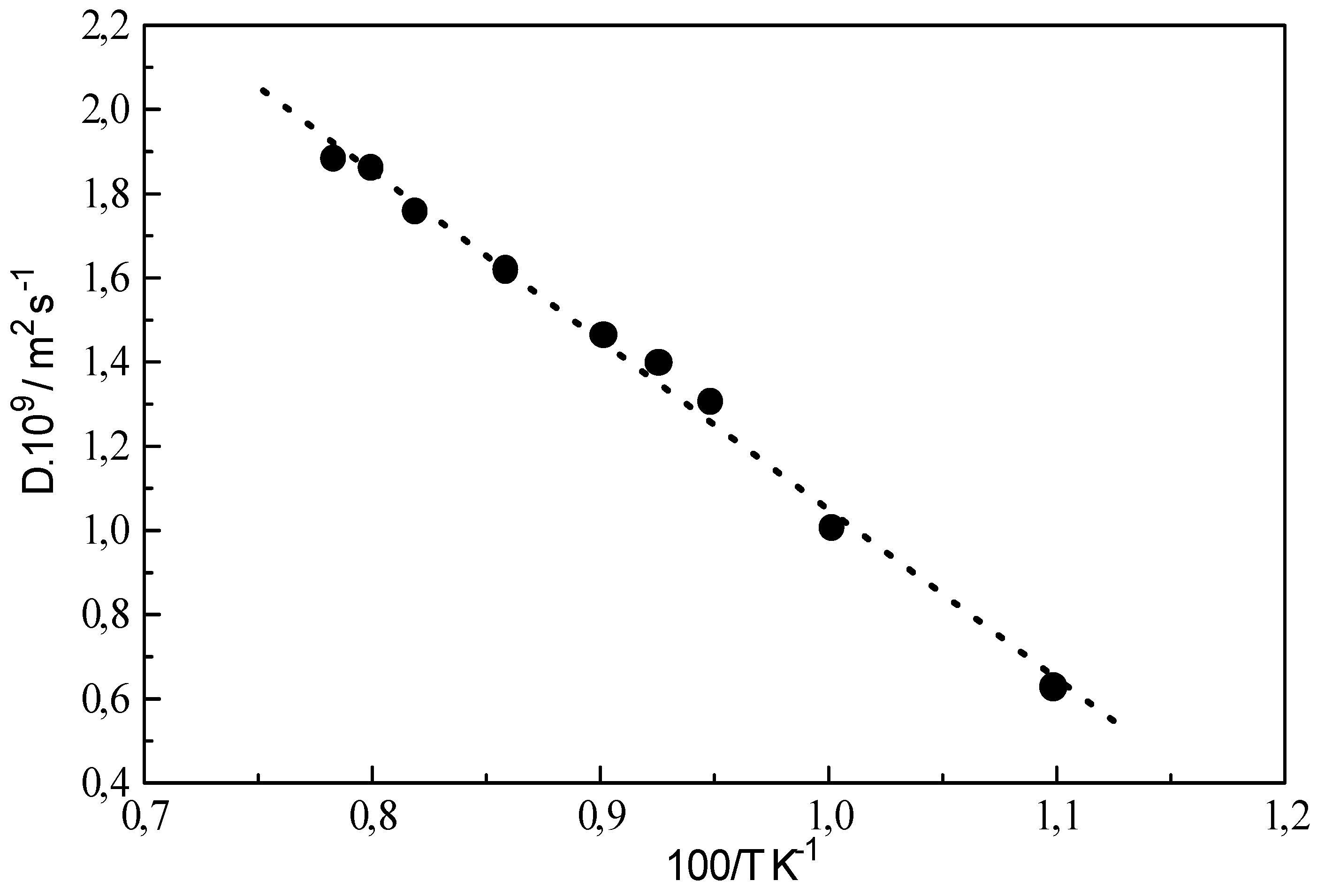
As expected, the shear viscosity decreases with increasing temperature. It is obvious that properties calculated at high temperatures and low densities require a correlation of collective transport properties over long simulation time. One can easily work out the activation energy from the diffusion coefficient versus temperature curve, using the Arrhenius low as illustrated in Figure 5. The calculated activation energy for methane is 3.34 K.J.mol^-1 and is found close to the activation energy measured by NMR (3.7 K.J.mol^-1) [35] and Schoen and al simulations [15] (3.2 K.J.mol^-1 with a spherical symmetric potential and 3.8 K.J.mol^-1 for centre site-site potential).

In order to obtain a complete analysis of our results and in order to demonstrate the reliability of classic model, a comparative study of our data with experimental [12,24,27] and theoretical works[3,12,27] is performed as reported by Table 3. For this purpose, we have reported data obtained by Sesé [3,12,27] from Monte-Carlo simulation involving Feynmann-Hibbs effective potential methods; Quadratic (QFH) and Gaussian(GFH) or the path-integral method (PIMC, PIBD, PIBC, MS-PI). A good agreement is found with the quantum approach except data of reference [3] using WK(h2). The pressure value shows the chronological order: PIMC > QFH ≅ WK ≅ MCLJ > DMLJ. The FH quantum effects and PIBC method increase total and potential energies as compared with classical LJ values. On the other hand, the three methods give completely different pressures. From all these results, one can draw the following observations: with decreasing densities, (a) the FH methods lead to thermodynamic properties remarkably close to experiment, (b) QFH and GFH approaches yield similar results, QFH being somewhat much more reliable. The agreement fails as the density increases, which can eventually lead to very poor estimates of some properties (pressure at Nesp4). The large pressure fluctuations make comparisons difficult to follow, nevertheless, pressures appear to be very large for quantum models when compared to classical model in agreement with Hansen and Weis[37], Thirumalai and Hall[36] and Singer and Smith[24].

Figure 5. Diffusion coefficient as a function of temperature for the pure liquid methane.

Figure 5. Diffusion coefficient as a function of temperature for the pure liquid methane.

Table 3. A Comparative study of data obtained with different investigations for liquid helium (Hesp1, hesp7), liquid methane (Msp1, Msp4, Msp8) and liquid neon (Nesp1-Nesp4). Experimental data are reported as well. Data are reported in reduced units.

	Method	U*	E*	P*
Hesp1	DMLJ(a)	-6.146 ±0.014	-5.845 ±0.012	-0.107 ±0.016
	QFH(b)	-4.195	-4.870	-0.341
	PIBC(b)	-2.135	-0.76	0.2
Hesp7	DMLJ(a)	-5.428 ±0.043	-4.677 ±0.043	-0.111 ±0.021
	QFH(b)	-2.655	-1.920	-0.220
	PIBC(b)	-2.07	-0.24	0.24
Msp1	Exp (c)		-5.526
	DMLJ(a)	-6.460 ± 0.059	-5.541 ± 0.112	0.024 ± 0.245
	MCLJ(b)	-6.493 ± 0.064	-5.577 ±0.064	0.190 ± 0.334
	WK(h2)(b)	-6.316 ± 0.064	-5.434 ±0.080	0.200 ± 0.279
	QFH(b)	-6.405 ± 0.067	-5.405 ±0.071	0.413 ± 0.348
	PIMC(b)	-6.408 ± 0.061	-5.413 ±0.278	0.396 ± 0.430
Msp4	Exp.(c)		-4.989
	DMLJ(a)	-6.049 ± 0.024	-4.962 ± 0.029	0.099 ± 0.116
	MCLJ(b)	-6.040 ± 0.067	-4.954 ± 0.067	0.122 ± 0.348
	WK(h2)(b)	-5.925 ± 0.071	-4.861 ± 0.086	0.214 ± 0.312
	QFH(b)	-6.003 ± 0.067	-4.851 ± 0.069	0.301 ± 0.338
	PIMC(b)	-6.000 ± 0.065	-4.853 ± 0.331	0.315 ± 0.484
Msp8	Exp.(c)		-4.416
	DMLJ(a)	-5.606 ± 0.026	-4.348 ± 0.026	0.162 ± 0.086
	MCLJ(b)	-5.604 ± 0.071	-4.347 ± 0.071	0.069 ± 0.345
	WK(h2)(b)	-5.517 ± 0.073	-4.274 ± 0.086	0.145 ± 0.311
	QFH(b)	-5.593 ± 0.068	-4.284 ± 0.071	0.104 ± 0.332
	PIMC(b)	-5.583 ± 0.070	-4.281 ± 0.375	0.170 ± 0.496
Nesp1	Exp.(c)	--	-4.37	-0.05
	DMLJ(a)	-5.923±0.017	-4.925±0.018	-0.587±0.079
	MCLJ(b)	-5.898±0.006	-4.900±0.006	-0.625±0.037
	QFH(b)	-5.739±0.011	-4.420±0.014	0.101±0.061
	GFH(b)	-5.699±0.013	-4.291±0.017	0.271±0.072
	MS-PI (b)	--	-4.50±0.030	-0.057±0.057
Nesp2	Exp.(c)	--	--	0.605
	DMLJ(a)	-5.091±0.022	-3.664±0.022	0.250±0.080
	MCLJ(b)	-5.270±0.008	-3.842±0.008	0.221±0.060
	QFH(b)	-5.159±0.008	-3.499±0.009	0.647±0.033
	GFH(b)	-5.145±0.010	-3.442±0.012	0.695±0.050
Nesp3	Exp.(c)	--	-3.3	0.341
	DMLJ(a)	-5.070±0.031	-3.643±0.031	0.279±0.102
	MCLJ(b)	-5.084±0.011	-3.656±0.011	-0.014±0.038
	QFH(b)	-4.984±0.005	-3.345±0.006	0.330±0.034
	GFH(b)	-4.967±0.005	-3.287±0.006	0.394±0.021
	MS-PI (b)	--	-3.390±0.003	0.290±0.094
Nesp4	Exp.(c)	--	--	0.093
	DMLJ(a)	-4.840±0.025	-3.411±0.028	-0.404±0.070
	MCLJ(b)	-4.832±0.007	-3.404±0.007	-0.217±0.036
	QFH(b)	-4.734±0.008	-3.118±0.009	0.051±0.025
	GFH(b)	-4.728±0.007	-3.076±0.009	0.091±0.032

a) Our workb) Taken from [3]-[12]c) Taken from [12]-[24]-[27].

Table 3. A Comparative study of data obtained with different investigations for liquid helium (Hesp1, hesp7), liquid methane (Msp1, Msp4, Msp8) and liquid neon (Nesp1-Nesp4). Experimental data are reported as well. Data are reported in reduced units.

	Method	U*	E*	P*
Hesp1	DMLJ(a)	-6.146 ±0.014	-5.845 ±0.012	-0.107 ±0.016
	QFH(b)	-4.195	-4.870	-0.341
	PIBC(b)	-2.135	-0.76	0.2
Hesp7	DMLJ(a)	-5.428 ±0.043	-4.677 ±0.043	-0.111 ±0.021
	QFH(b)	-2.655	-1.920	-0.220
	PIBC(b)	-2.07	-0.24	0.24
Msp1	Exp (c)		-5.526
	DMLJ(a)	-6.460 ± 0.059	-5.541 ± 0.112	0.024 ± 0.245
	MCLJ(b)	-6.493 ± 0.064	-5.577 ±0.064	0.190 ± 0.334
	WK(h2)(b)	-6.316 ± 0.064	-5.434 ±0.080	0.200 ± 0.279
	QFH(b)	-6.405 ± 0.067	-5.405 ±0.071	0.413 ± 0.348
	PIMC(b)	-6.408 ± 0.061	-5.413 ±0.278	0.396 ± 0.430
Msp4	Exp.(c)		-4.989
	DMLJ(a)	-6.049 ± 0.024	-4.962 ± 0.029	0.099 ± 0.116
	MCLJ(b)	-6.040 ± 0.067	-4.954 ± 0.067	0.122 ± 0.348
	WK(h2)(b)	-5.925 ± 0.071	-4.861 ± 0.086	0.214 ± 0.312
	QFH(b)	-6.003 ± 0.067	-4.851 ± 0.069	0.301 ± 0.338
	PIMC(b)	-6.000 ± 0.065	-4.853 ± 0.331	0.315 ± 0.484
Msp8	Exp.(c)		-4.416
	DMLJ(a)	-5.606 ± 0.026	-4.348 ± 0.026	0.162 ± 0.086
	MCLJ(b)	-5.604 ± 0.071	-4.347 ± 0.071	0.069 ± 0.345
	WK(h2)(b)	-5.517 ± 0.073	-4.274 ± 0.086	0.145 ± 0.311
	QFH(b)	-5.593 ± 0.068	-4.284 ± 0.071	0.104 ± 0.332
	PIMC(b)	-5.583 ± 0.070	-4.281 ± 0.375	0.170 ± 0.496
Nesp1	Exp.(c)	--	-4.37	-0.05
	DMLJ(a)	-5.923±0.017	-4.925±0.018	-0.587±0.079
	MCLJ(b)	-5.898±0.006	-4.900±0.006	-0.625±0.037
	QFH(b)	-5.739±0.011	-4.420±0.014	0.101±0.061
	GFH(b)	-5.699±0.013	-4.291±0.017	0.271±0.072
	MS-PI (b)	--	-4.50±0.030	-0.057±0.057
Nesp2	Exp.(c)	--	--	0.605
	DMLJ(a)	-5.091±0.022	-3.664±0.022	0.250±0.080
	MCLJ(b)	-5.270±0.008	-3.842±0.008	0.221±0.060
	QFH(b)	-5.159±0.008	-3.499±0.009	0.647±0.033
	GFH(b)	-5.145±0.010	-3.442±0.012	0.695±0.050
Nesp3	Exp.(c)	--	-3.3	0.341
	DMLJ(a)	-5.070±0.031	-3.643±0.031	0.279±0.102
	MCLJ(b)	-5.084±0.011	-3.656±0.011	-0.014±0.038
	QFH(b)	-4.984±0.005	-3.345±0.006	0.330±0.034
	GFH(b)	-4.967±0.005	-3.287±0.006	0.394±0.021
	MS-PI (b)	--	-3.390±0.003	0.290±0.094
Nesp4	Exp.(c)	--	--	0.093
	DMLJ(a)	-4.840±0.025	-3.411±0.028	-0.404±0.070
	MCLJ(b)	-4.832±0.007	-3.404±0.007	-0.217±0.036
	QFH(b)	-4.734±0.008	-3.118±0.009	0.051±0.025
	GFH(b)	-4.728±0.007	-3.076±0.009	0.091±0.032

a) Our workb) Taken from [3]-[12]c) Taken from [12]-[24]-[27].

From this Table 3, it appears also that the basic three methods compared (classical Molecular Dynamics, quantum Monte-Carlo and path-integral computation) deviate very strongly from each other for the case of Helium, where they show random behavior, while they lead to fairly consistent results for methane. This suggests that none of the methods succeeds in capturing the strong quantum effects that are characteristic for liquid Helium. All these approaches are semi classical finite-temperature techniques, which may provide a measure of improvement over quantum-corrected classical results (liquid neon), but which are not applicable in the strongly quantum-mechanical low-temperature limit (liquid helium) [38,39].

Conclusion

Classical molecular dynamics simulation of Lennard Jones fluids is possible within different state point of the phase diagram. Lennard-Jones liquid energies are not affected by translational quantification because the static errors in the quantum models explain the experimental data. This is the Lennard-Jones fitting consequence [2] witch take into account one way or the other quantum effects. Quantum effects are necessary to explain the different behaviour near the triple point. Our work offers the possibility to study the transport properties with a good precision as for the diffusion coefficient or the shear viscosity. Our results compare favorably with both experiment and more sophisticated theoretical approaches that incorporate quantum effects.