Introducing Spectral Structure Activity Relationship (S-SAR) Analysis. Application to Ecotoxicology

Abstract

A novel quantitative structure-activity (property) relationship model, namely Spectral-SAR, is presented in an exclusive algebraic way replacing the old-fashioned multi-regression one. The actual S-SAR method interprets structural descriptors as vectors in a generic data space that is further mapped into a full orthogonal space by means of the Gram-Schmidt algorithm. Then, by coordinated transformation between the data and orthogonal spaces, the S-SAR equation is given under simple determinant form for any chemical-biological interactions under study. While proving to give the same analytical equation and correlation results with standard multivariate statistics, the actual S-SAR frame allows the introduction of the spectral norm as a valid substitute for the correlation factor, while also having the advantage to design the various related SAR models through the introduced “minimal spectral path” rule. An application is given performing a complete S-SAR analysis upon the Tetrahymena pyriformis ciliate species employing its reported eco-toxicity activities among relevant classes of xenobiotics. By representing the spectral norm of the endpoint models against the concerned structural coordinates, the obtained S-SAR endpoints hierarchy scheme opens the perspective to further design the ecotoxicological test batteries with organisms from different species.

1. Introduction

In Chemistry, the first systematic correlations come from Lavoisier’s law of conservation of mass and energy, followed by the Dalton conception of structural matter. Nevertheless, Mendeleyev was the first one to place the structure-activity relationships (SARs) in the centre of chemistry with his vision of the periodic table [1]. However, with the advent of quantum theory, the relations among elements of periods and down groups of periodic table acquired in-depth quantitative meaning, by relating the elementary electronic structure with the manifested atomic reactivity through, for instance, basic electronegativity and chemical hardness indices [2,3]. This way, it appears that every aspect of chemical reactivity can be seen as a certain manifestation of the structure-property pair that is quantified since the derivation of the associated equation [4].

Yet, the current problem of science is to organize the huge amount of experimental information in comprehensive equations with a predictive value. At this point, the quantitative structure-activity relationships (QSARs) methods seem to offer the best key for unifying the chemical and biological interaction into a single in vivo-in vitro content [5–10].

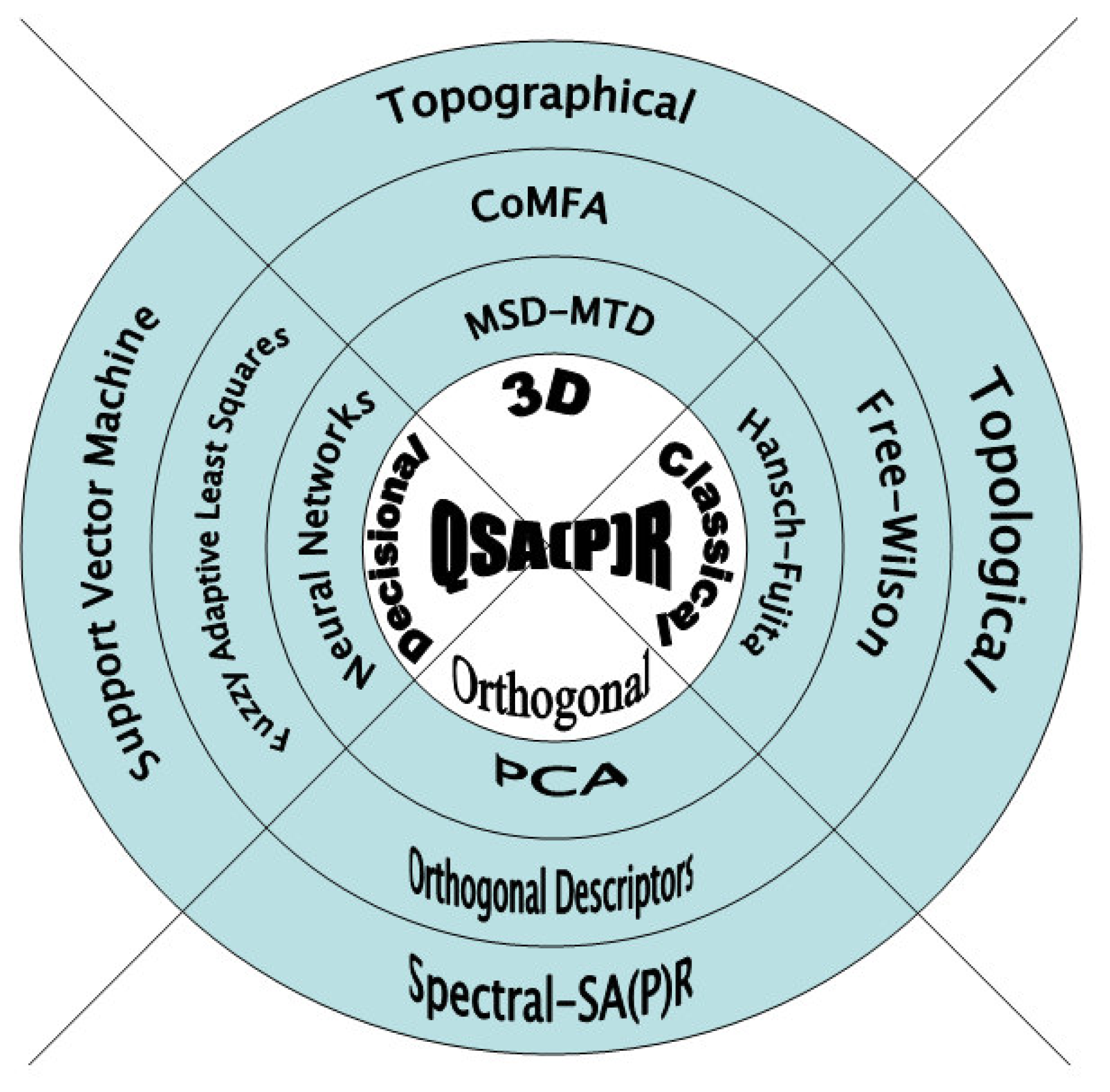
However, although the main purpose of QSARs studies is all about finding structural parameters that best correlate with the activity/property of the interactions observed, a multitude of methods of attaining this goal have appeared. They struggle to identify the most appropriate manner of quantifying the causes in such a way that they may be reflected in the measurement with maximal accuracy or minimal error. Phenomenologically, these methods can be conceptually grouped into “classical” [11–19], “3-dimensional” [20–30], “decisional” [31–42], and “orthogonal” ones [43–57], together represented as in Figure 1.

In short, classic QSAR approaches assume as descriptors the structural indices that directly reflect the electronic structures of the tested chemical compounds. As such, they assume that the biological activity depends on factors describing the lipophylicity (e.g. LogP, surfaces), electronic effects (e.g. Hammett constants, polarization, localization of charges), and steric effects (e.g. Taft indices, Verloop indices, topological indices, molecular mass, total energy at optimized molecular geometry) [12, 13].

A step forward is made when 3-dimensional structures are characterized by entry indices. For instance, the MTD (minimal topological difference) [23–25] and CoMFA (comparative molecular field analysis) [26, 27] methods are closely take into account the bioactive conformation of the receptor, the topology of the ligand series as well as their steric fit, in accordance with the “key-into-lock” principle, while the topographical schemes [29, 30] make use of the graph representation of the chemical compounds, replacing in the associated connectivity matrices the optimized stereochemical indices. A visible increase in the structure-activity correlation is usually recorded when these methods are used [28].

Still, statistically, it was found that in order for multiple linear regressions to be used, the requirement of a large number of compounds has to be met in order to explore the structural combination. Under these circumstances, the next QSARs category in Figure 1, namely the decisional one appears as further natural approach. Basically, they are heuristic methods of classifying data, developing genetic algorithms, i.e. neural networks [31,32], fuzzy methodologies [34,35], or support vector machine for learning [36–42], in order to find optimal solutions for combinatorial problems. They offer the advantage of providing a quick estimation regarding the quality of correlation we should expect from the data and furnishing several best regression models to decide upon. Moreover, the decisional analysis can be made in high-dimensional space always giving a solution by standard algorithm.

Nevertheless, despite having several solutions to decide over thousands of products from millions of libraries, together with hundred descriptors, that opens the problem of their further relevance and classification. With these we have arrived at the heart of a QSAR analysis: the orthogonal problem. Statistically, this term was interpreted as descriptors whose values form a basis set that pose little intercorrelation factors. In practice, data reduction techniques such as PCA (principal component analysis) [43,45] describe biological activity or chemical properties through a fewer number of independent (orthogonal) descriptors giving a regression equation on these principal components. Unfortunately, even combined with PLS (partial least squares) cross-validation technique to produce higher predictive QSAR models, the main drawback still remains since they furnish scarce possibility to interpret the obtained models [44,46].

Another way of interpreting orthogonality was given through producing an orthogonal space by transforming the original basis set of descriptors in an orthogonal one by searching of inter-regression equations between them [47], followed, eventually, by their reciprocal subtractions [48]. Unfortunately, this method was found to give in almost all cases the same correlation and statistical factors as those furnished by regressions with original basis set of descriptors [49–54], moreover, producing a QSAR equation in the orthogonal space where the orthogonal descriptors have little interpretation against the real ones. At the end, the orthogonal descriptors’ method becomes another technique for selecting the independent predictor variables (like PCA) rather than one that provides alternative solution for basic SAR problem [55].

Under these circumstances, the third attempt of interpreting the orthogonal problem is considering the scalar product as the main vehicle in releasing the QSAR solution in a completely algebraic way thus furnishing the so called Spectral-SAR (S-SAR) technique in Figure 1 for reasons revealed bellow. It is based on the employment of the generalized Euclidian scalar product rule among the vectors associated to the descriptors’ data in a way that produce, thought the Gram-Schmidt algorithm and coordinate transformation, precisely the same results as the statistical multi linear regression techniques do. This new QSAR method, initiated in a relatively limited dissemination space [56,57], is presented in full here, while also giving its equivalence with the standard multiple linear regression method. Nevertheless, the features of the present S-SAR method include some of its predecessor’s, including vectorial frame and output, high-dimensionality for the data space, adaptive analysis, showing, however, independence concerning the order of orthogonal vectors and also proving the spectral norm as an alternative algebraic tool for substituting of the statistical correlation factor.

The field of ecotoxicology was chosen as an application, where various combined S-SAR-Hansch models are constructed for describing the toxicity of 26 xenobiotics on the Tetrahymena pyriformis species. It follows that S-SAR approach gives the specific algebraic tool, i.e. the spectral norm, with which the specific ecotoxicological endpoint concept acquires new feasible degree. The present S-SAR analysis leaves room for other similar studies when it is joined with other classical, 3-dimensional and decisional QSAR techniques of Figure 1 so contributing to unite the chemical-biological interactions in a veritable QSAR science.

2. The Spectral-SAR Method

2.1. Background Concepts

The basic problem of structure-activity relationship analysis can be formulated as follows: given a set of measured activities of a certain series of (say N) compounds, the optimal correlation between these activities and the structural (internal, intrinsic) properties of the compounds (say M properties) is sought, according to

Table 1. Synopsis of the basic SAR descriptors.

Activity	Structural predictor variables
y1	x11	…	x1k	…	x1M
y2	x21	…	x2k	…	x2M
⋮	⋮	⋮	⋮	⋮	⋮
yN	xN1	…	xNk	…	xNM

, in the form of the general multi-linear equation:

$$y=b_0+b_1{x}_1+\dots +b_k{x}_k+\dots +b_M{x}_M+e.$$

(1)

In equation (1)y represents the generic activity in relation with an arbitrary set of independent variables x_i, i=1, …, M through the fixed parameters b_j, j=0, …, M, while e stands as the residual or error value between the assumed multi-linear model and measurements.

Therefore, the SAR problem becomes quantitative since the set of fixed parameters is determined so that the errors in activity evaluation are minimized. This way, the equation (1) may be used to predict the activity (without experimental measurement) for each further input of the structural parameters.

However, this “Holy Grail” property of a QSAR equation opens the issue of significance and statistical relevance of the values considered in Table 1, as well as that of the computational method by which the parameters of (1) are assessed.

Usually, the QSAR problem is solved in the so called “normal or “standard” way, briefly described in what follows. Firstly, the equation (1) is particularized for each activity entry of Table 1 thus generating the N×(M+1) system:

$$\begin{array}{c}{y}_1=b_0+b_1{x}_{11}+\dots +b_k{x}_{1k}+\dots +b_M{x}_{1M}+e_1\\ y_2=b_0+b_1{x}_{21}+\dots +b_k{x}_{2k}+\dots +b_M{x}_{2M}+e_2\\ ⋮\\ y_N=b_0+b_1{x}_{N1}+\dots +b_k{x}_{Nk}+\dots +b_M{x}_{NM}+e_N\end{array}$$

(2)

Note that, generally, each activity evaluation is assumed to be accompanied by a different error, i.e. the values e₁, …, e_N are potentially different although the ideal case would demand that they be equal with zero.

However, since the following matrices are introduced

$$Y=\left(\begin{array}{l}{y}_1\hfill \\ y_2\hfill \\ ⋮\hfill \\ y_N\hfill \end{array}\right),E=\left(\begin{array}{l}{e}_1\hfill \\ e_2\hfill \\ ⋮\hfill \\ e_N\hfill \end{array}\right),B=\left(\begin{array}{l}{b}_0\hfill \\ b_1\hfill \\ b_2\hfill \\ ⋮\hfill \\ b_M\hfill \end{array}\right),X=\left(\begin{array}{lllll}1\hfill & x_{11}\hfill & x_{12}\hfill & \cdots \hfill & x_{1M}\hfill \\ 1\hfill & x_{21}\hfill & x_{22}\hfill & \cdots \hfill & x_{2M}\hfill \\ ⋮\hfill & ⋮\hfill & ⋮\hfill & ⋮\hfill & ⋮\hfill \\ 1\hfill & x_{N1}\hfill & x_{N2}\hfill & \cdots \hfill & x_{NM}\hfill \end{array}\right),$$

(3)

the system (2) can be rewritten in a simple algebraic way:

$$Y=XB+E.$$

(4)

Hence, the minimization of the error vector E equals the minimization of the vector (Y-XB) in (4).

Put in vectorial terms, the solution of the supra-dimensional system (2) is a vector φ (B) which minimizes the Euclidian norm of the residual (error) vector, in a least square sense:

$$\phi (B)={(Y-XB)}^T(Y-XB)\to \text{min}.$$

(5)

Finally, one uses the following theorem [58–61]: if the vector B of (3) is the solution of the linear system (6),

$$X^T(Y-XB)=0,$$

(6)

where X is a real matrix of dimension N×(M+1) and B a vector of dimension (M+1)×1, then the standard deviation of XB with respect to Y is minimal, i.e. the condition (5) is fulfilled.

This means that we can consider norm(E)→0 when relations (4) and (6) are combined to give the B vector of estimates

$$B={\left(X^{T}X\right)}^{-1}{X}^{T}Y.$$

(7)

It is worth noting that while solution (7) solves the above QSAR problem in a formal way the concrete application of this method requires a high computational effort even when the symmetry of the matrix X^TX is taken into account.

Despite this, the “normal” or “standard” QSAR procedure is already implemented in various software packages nowadays. It is worth exploring other alternative way that may serve both conceptual and computational advantages. The so called “spectral” algorithm, presented below, stands as such a new perspective, belonging to “orthogonal QSAR” methods of Figure 1.

2.2. Spectral-SAR Algorithm

The key concept in SAR discussion regards the independence of the considered structural parameters in Table 1. As a consequence we may further employ this feature to quantify the basic SAR through an orthogonal space.

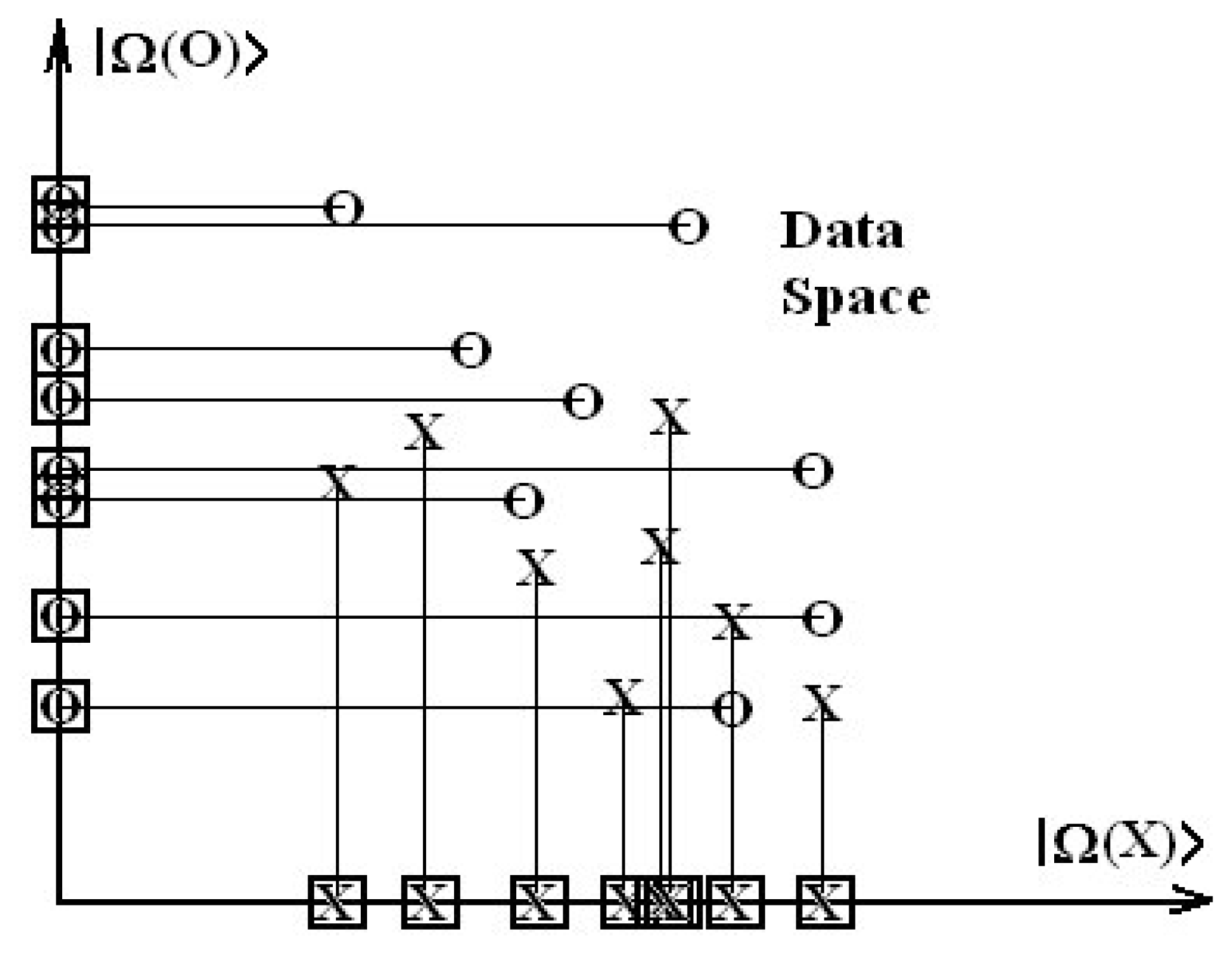
The idea is to transform the columns of structural data of Table 1 into an abstract orthogonal space, where necessarily all predictor variables are independent, see Figure 2; solve the SAR problem there and then referring the result to the initial data by means of a coordinate transformation.

The analytical procedure is unfolded in simple tree steps.

Basically, Table 1 is reconsidered under the form of

Table 2. The spectral (vectorial) version of SAR descriptors of Table 1.

Activity	Structural predictor variables
|Y〉	|X0〉	|X1〉	…	|Xk〉	…	|XM〉
y1	1	x11	…	x1k	…	x1M
y2	1	x21	…	x2k	…	x2M
⋮	⋮	⋮	⋮	⋮	⋮	⋮
yN	1	xN1	…	xNk	…	xNM

where, for completeness, the unity column has been added |X₀〉 = |1 1... 1〉 for accounting of the coefficients of the free term (b₀) of system (2).

Moreover, since the columns are now considered as vectors in data space we are looking for the “spectral” decomposition of the activity vector |Y〉 upon the considered basis of the structural vectors {X₀〉, |X₁〉,..., |X_k〉,..., |X_M〉}:

$$\mid Y\rangle =b_0\mid X_0\rangle +b_1\mid X_1\rangle +\dots +b_k\mid X_k\rangle +\dots +b_M\mid X_M\rangle +\mid e\rangle .$$

(8)

Equation (8) stands, in fact, as a spectral decomposition counterpart of the multi-linear equation (1), equation that the name of the present approach comes from.

The next step is to construct a vectorial algorithm so that the residual vector |e〉 can be sent to zero in (8) in order to fulfill the above (5) condition of minimizing of errors.

To achieve the minimal errors in (8) the transformation of the data basis {|X₀〉, |X₁〉,..., |X_k〉,..., |X_M〉} into an orthogonal one, say {|Ω₀〉, |Ω₁〉,..., |Ω_k〉,..., |Ω _M〉}, is now considered. In this respect the consecrated Gram-Schmidt procedure is employed. It is worth noting that this procedure is well known in quantum chemistry when searching for an orthogonal basis for an orthogonal basis set in atomic and molecular wave function spectral decomposition [62].

However, before applying it effectively one has to introduce the generalized scalar product throughout the basic rule:

$$\langle {\mathrm{\Psi }}_l\mid {\mathrm{\Psi }}_k\rangle =\sum _{i=1}^N{\psi }_{il}{\psi }_{ik}=\langle {\mathrm{\Psi }}_k\mid {\mathrm{\Psi }}_l\rangle$$

(9)

giving out a real number from two arbitrary N-dimensional vectors

$$\mid {\mathrm{\Psi }}_l\rangle =\mid \begin{array}{cccc}{\psi }_{1l}& {\psi }_{2l}& \dots & {\psi }_{Nl}\end{array}\rangle ,\mid {\mathrm{\Psi }}_k\rangle =\mid \begin{array}{cccc}{\psi }_{1k}& {\psi }_{2k}& \dots & {\psi }_{Nk}\end{array}\rangle .$$

Briefly, remember that the orthogonal condition requires that the scalar product of type (9) to be zero, the orthogonal basis {|Ω₀〉, |Ω₁〉,..., |Ω_k〉,..., |Ω _M〉}, can be constructed from the set {|X₀〉, |X₁〉,..., |X_k〉,..., |X_M〉} according with the iterative recipe:

• Choose
  $$\mid {\mathrm{\Omega }}_0\rangle =\mid X_0\rangle ;$$

  (10)
• Then, by picking |X₁〉 as the next vector to be transformed, one can write that:
  $$\mid {\mathrm{\Omega }}_1\rangle =\mid X_1\rangle -r_0^1\mid {\mathrm{\Omega }}_0\rangle ,\hspace{0.17em}{r}_0^1=\frac{\langle X_1\mid {\mathrm{\Omega }}_0\rangle }{\langle {\mathrm{\Omega }}_0\mid {\mathrm{\Omega }}_0\rangle }$$

  (11)
  so that 〈Ω₀|Ω₁〉 = 0 assuring so far that |Ω₀〉 and |Ω₁〉 are orthogonal.
• Next, repeating steps i. and ii. above until the vectors |Ω₀〉, |Ω₁〉, …, |Ω_k−1〉 are orthogonally constructed, we can, for instance, further transform the vector |X_k〉 into :
  $$\mid {\mathrm{\Omega }}_k\rangle =\mid X_k\rangle -\sum _{i=0}^{k-1}{r}_i^k\mid {\mathrm{\Omega }}_i\rangle ,\hspace{0.17em}{r}_i^k-\frac{\langle X_k\mid {\mathrm{\Omega }}_i\rangle }{\langle {\mathrm{\Omega }}_i\mid {\mathrm{\Omega }}_i\rangle }$$

  (12)
  so that the vector |Ω_k〉 is orthogonal on all previous ones.
• Step (iii) is repeated and extended until the last orthogonal predictor vector |Ω_M〉 is obtained.

Therefore, grounded on the Gram-Schmidt recipe the starting predictor vectorial basis {|X₀〉, |X₁〉,..., |X_k〉,..., |X_M〉}is replaced with the orthogonal one {|Ω₀〉, |Ω₁〉,..., |Ω_k〉,..., |Ω _M〉} by appropriately subtracting from the original vectors the non-wished non-orthogonal contributions. Note that the above procedure holds for any arbitrary order of original vectors to be orthogonalized.

Within the constructed orthogonal space, the vector activity |Y〉 achieves true spectral decomposition form:

$$\mid Y\rangle ={\omega }_0\mid {\mathrm{\Omega }}_0\rangle +{\omega }_1\mid {\mathrm{\Omega }}_1\rangle +\dots +{\omega }_k\mid {\mathrm{\Omega }}_k\rangle +\dots +{\omega }_M\mid {\mathrm{\Omega }}_M\rangle .$$

(13)

Note that the residual vector in equation (8) has disappeared in (13) since it has no structural meaning in the abstracted orthogonal basis. Or, alternatively, one can say that in the abstract orthogonal space the residual vector |e〉 was identified with the vector with all components zero |0,0,...,0〉 that is always perpendicular with all other vectors of orthogonal basis.

This way, the Gram-Schmidt algorithm, by its specific orthogonal recursive rules, absorbs or transforms the minimization condition of errors in (8) to simple identification with the origin of the orthogonal space of data.

At this point, since there is no residual vector remaining in (13) one can consider that the SAR problem is in principle solved once the new coefficients in (13) (ω₀, ω₁,...,ω_k,...,ω _M ) are determined. These new coefficients can be immediately deduced based on the orthogonal peculiarities of the spectral decomposition (13) grounded on the fact that:

$$\langle {\mathrm{\Omega }}_k\mid {\mathrm{\Omega }}_l\rangle =0\hspace{0.17em},\hspace{0.17em}k\ne l,$$

(14)

a condition assured by the very nature of the vectors from the constructed orthogonal basis.

As such, each coefficient comes out as the scalar product of its specific predictor vector with the activity vector (13) is performed:

$${\omega }_k=\frac{\langle {\mathrm{\Omega }}_k\mid Y\rangle }{\langle {\mathrm{\Omega }}_k\mid {\mathrm{\Omega }}_k\rangle },\hspace{0.17em}k=\overline{0,M}.$$

(15)

With coefficients given by expressions of type (15) the spectral expansion of the activity vector into an orthogonal basis (13) is completed. Yet, this does not mean that we have found the coefficients that directly link the activity with the predictor vectors as equation (8) demands.

However, this goal is easily achieved through the final stage of the present SAR algorithm. It consists in going back from the orthogonal to the initial basis of data through the system of coordinate transformations:

$$\{\begin{array}{l}\mid Y\rangle ={\omega }_0\mid {\mathrm{\Omega }}_0\rangle +{\omega }_1\mid {\mathrm{\Omega }}_1\rangle +\dots +{\omega }_k\mid {\mathrm{\Omega }}_k\rangle +\dots +{\omega }_M\mid {\mathrm{\Omega }}_M\rangle \hfill \\ \mid X_0\rangle =1·\mid {\mathrm{\Omega }}_0\rangle +0·\mid {\mathrm{\Omega }}_1\rangle +\dots +0·\mid {\mathrm{\Omega }}_k\rangle +\dots +0·\mid {\mathrm{\Omega }}_M\rangle \hfill \\ \mid X_1\rangle =r_0^1\mid {\mathrm{\Omega }}_0\rangle +1·\mid {\mathrm{\Omega }}_1\rangle +\dots +0·\mid {\mathrm{\Omega }}_k\rangle +\dots +0·\mid {\mathrm{\Omega }}_M\rangle \hfill \\ \mid X_k\rangle =r_0^k\mid {\mathrm{\Omega }}_0\rangle +r_1^k\mid {\mathrm{\Omega }}_1\rangle +\dots +1·\mid {\mathrm{\Omega }}_k\rangle +\dots +0·\mid {\mathrm{\Omega }}_M\rangle \hfill \\ \mid X_M\rangle =r_0^M\mid {\mathrm{\Omega }}_0\rangle +r_1^M\mid {\mathrm{\Omega }}_1\rangle +\dots +r_k^M\mid {\mathrm{\Omega }}_k\rangle +\dots +1·\mid {\mathrm{\Omega }}_M\rangle \hfill \end{array}$$

(16)

While the first equation of (16) reproduces the entire spectral decomposition (13), the rest of them are convenient rewritings of the Gram-Schmidt transformations (10)-(12).

Finally, the system (16) is algebraically true if and only if the associated augmented determinant disappears,

$$\left|\begin{array}{ccccccc}\mid Y\rangle & {\omega }_0& {\omega }_1& \cdots & {\omega }_k& \cdots & {\omega }_M\\ \mid X_0\rangle & 1& 0& \cdots & 0& \cdots & 0\\ \mid X_1\rangle & r_0^1& 1& \cdots & 0& \cdots & 0\\ ⋮& ⋮& ⋮& ⋮& \hspace{0.17em}& ⋮& \hspace{0.17em}\\ \mid X_k\rangle & r_0^k& r_1^k& \cdots & 1& \cdots & 0\\ ⋮& ⋮& ⋮& ⋮& \hspace{0.17em}& ⋮& \hspace{0.17em}\\ \mid X_M\rangle & r_0^M& r_1^M& \cdots & r_k^M& \cdots & 1\end{array}\right|=0,$$

(17)

this being the condition consecrated by the theorem according to which a system possessing a column as a linear combination of all others has a zero allied determinant[58].

It is worth noting that the minimization of residual errors was unnecessarily complicated in previous orthogonalization approaches [54] by involving standard multi-linear regressions, iteratively, among the selected structural descriptors and of their combination [53]. This way, the flavor of performing an alternative orthogonal approach of the SAR issue was lost in an ocean of inter-correlations. Consequently, the heuristic methods used in the search for an orthogonal set of descriptors, in the regression sense, though an arbitrarily minimal inter-correlation factors, leave both the realistic meaning of the usually lesser set of orthogonalized descriptors, as compared with the original one, and the initial SAR problem to be solved. On the contrary, within the present orthogonal endeavor, the Spectral-SAR method proposes a new way of completely solving of a SAR problem linking the measured activities (or observed properties) with the structural descriptors in a simpler and more transparent algebraic way than the “standard” multi-linear regression method do.

Moreover, the ordering problem in all previous orthogonal descriptors’ methods [54] is eliminated with the present S-SAR analysis since all structural descriptors are spectrally expanded at once complying with the orthogonal basis, as Eq. (16) reveals, avoiding iterative reciprocal correlations among orthogonal descriptors where their considered order becomes essential. This special feature of S-SAR will be illustrated later, in the application section.

It is now clear that once expanded, observing its first column, the determinant (17) generates the searched full solution of the basic SAR problem of Table 2 with minimization of errors included and independent of the orthogonalization order. Remarkably, apart from being conceptually new through considering the spectral (orthogonal) expansion of the input data space (of both activity and descriptors) through the system (16), the present method also has the computational advantage of being simpler than the classical “standard” way of treating SAR problem previously exposed. That because, one has nothing to do with computations of matrix of the coefficients (7), this being a quite involving and time consuming procedure. Instead, one can write directly the spectral-SAR solution (equation) as the expansion of a (M+2)-dimensional determinant of type (17) whose components are the activity and structural vectors among the Gram-Schmidt and the spectral decomposition coefficients, $r_k^l$ and ω_k, respectively.

However, although different from the mathematical procedure, both standard- and spectral-SAR give similar results due to the theorem that states that [61]: if the matrix X, as that from (3), with dimension N×(M+1), N>M+1, has linear independent columns, i.e. they are orthogonal as in the spectral approach, then there exists an unique matrix Q of dimension N×(M+1) with orthogonal columns and a triangular matrix R of dimension (M+1)×(M+1) with the elements of the principal diagonal equal with 1, as identified in the first small determinant in (17), so that the matrix X can be factorized as

$$X=QR.$$

(18)

When combining equation (18) with the optimal equation (6) one can get, after straight algebraic rules, that the B vector of estimates takes the form

$$B={\left(Q^{T}Q\right)}^{-1}{Q}^{T}Y,$$

(19)

in close agreement with previous normal one, see equation (7). However, by comparison of matrices X^TX and Q^TQ in equations (7) and (19), respectively, there is clear that the last case certainly furnishes a diagonal form which for sure is easier to handle (i.e. to take its inverse) when searching for the vector B of SAR coefficients.

With these considerations one would prefer the present Spectral-SAR approach when solving the QSAR problems in chemistry and related molecular fields. Nevertheless, wishing to also provide a practical advantage of the exposed Spectral-SAR scheme, a specific application, with relevance in ecotoxicological studies, is presented in the next section.

3. Application to Ecotoxicology

3.1 Basic Characteristics of QSAR in Ecotoxicology

From more than one decade the European Union institutions, e.g. Organization for Economic Cooperation and Development (OECD) through its Registration, Evaluation, and Authorization of Chemicals (REACH) management system [63, 64], the United States Environmental Protection Agency (EPA) as part of the premanufactory notification assessment, as well as the World Health Organization have been developing impressive programs on the regulatory assessment of chemical safety by using of the QSAR data bases and of the associated automated expert systems [65–73]. This because, with the tones of chemicals that force their way onto the market each year and due to their commercial and industrial disposal into the environment, it becomes of first importance to predict their toxicological activities from the molecular structure in order to properly design the risk assessment measures [67–77].

Nevertheless, in order to best accomplish such a goal, both a conceptual and a computational strategy need to be adopted. As such, while, for instance, a certain set of parameters has been identified for environmental studies, i.e. bioaccumulation, chemical degradation (aqueous and gas phase), biodegradation, soil sorption, and ecotoxicity, two major aspects have been identified for QSAR analyses, namely the quality and the chemical domain of the QSAR [69,71,72].

Concerning the parameters to be evaluated, they are analytically transposed into the so called endpoints, representing specific experimental and measurement quantities giving information about the environmental risk degree. They are thus identified with the QSAR activities (biophores or toxicophores) to be correlated and are usually expressed as log-based continuous toxicological data (e.g. median lethal concentration-LC₅₀, 50% effect concentration-EC₅₀, 50% grow inhibition concentration-IGC₅₀) [74–77].

On the other hand, a useful QSAR model has to satisfy selection criteria in order to be validated.

From the statistical point of view the ratio of data points to the number of variables should be higher or equal to 5 (the so called Topliss-Costello rule [78]) and to provide a correlation factor r > 0.84.

As descriptors, those directly related to molecular structure of chemical are preferable. It is worth noting here that the quantum chemical parameters have an advantage against those of topological nature; still the quantum parameters to be used has to be relatively easily obtainable, for instance those based on ground state or valence state properties of compounds are preferable to those based on transition-state calculations [10].

If descriptors are taken from experiments, the experimental conditions must be specified. Nevertheless, the best models predicting ecotoxic effects have to be mechanistic interpretable, though that structure-activity correlation permits reconstruction or prediction of the basic phenomena that take place at the molecular level.

Regarding the outliers they have to be treated with caution, as they are not necessarily outside of the chemical domain but depending on the QSAR model (i.e. of the correlated descriptors) employed [79]. Moreover, the atypical data (presumed outliers) may represent compounds acting by a different mechanism, inducing an inhibition or belonging to dissimilar chemical structure. However, they should not be excluded from an analysis unless relevant alternative QSAR models were constructed. With this issue, we arrive at the chemical domain problem or at the representative set of compounds for the QSAR analysis.

Based on previous criteria in order for a QSAR analysis to be well conducted, a compromise between breath (variety) and depth (representability) characteristics through the existing chemicals within that domain have to be considered.

This way, the two-fold process of dissimilarity- and similarity- based selection is achieved [10]. The motivation for this criteria is that, while similar compounds (usually based on substitutions) assures the basic congenericity QSAR condition, considering dissimilar chemicals can predict how (however subtle) alterations in molecular structure can lead to changes in the mechanism of toxicity action and potency in the tested series of compounds. In short, this condition can be regarded as structural heterogeneity of compounds.

After all, it is widely recognized that ecotoxicity action is a multivariate process involving xenobiotics leading with immediate and long-term effects due o various transformations products. Therefore, a QSAR approach may provide information of the bio-up-take (i.e. of key process) through the selected descriptors that can be integrated in an expert system of toxic prediction.

However, with a view to designing an ecotoxicological mechanistic battery for different species on QSAR grounds, the first stage of unicellular organism level is undertaken here.

3.2 Bio-ecological Issues of Unicellular Organisms

We often think of unicellular organisms as having a simple, primitive structure. This is definitely an erroneous view when applied to the ciliates; they are probably the most complex of all unicellular organisms.

Unlike multicellular organisms, which have cells specialized for performing the various body functions, single-celled organisms must perform all these functions with a single cell, and so their structure may be much more complex than the cells of larger organisms.

Movement, sensitivity to the environment, water balance, and food capture must all be accomplished with the machinery in a single cell [80,81a–d]. As protozoans these organisms are classified according to their means of locomotion: by cilia (Ciliophora), flagella (Sarcomastigophora), or pseudopodia (Rhizopoda), while non-motile protists are classified as sporozoans in the phylum Apicomplexa.

Many of these single-celled organisms feed by engulfing smaller organisms directly into temporary intracellular vacuoles. These food vacuoles circulate in a characteristic manner within the cells while enzymes are secreted into them for digestion [81b].

However, form the taxonomy points of view they are classified downwards, from kingdom to species as: Protista > Ciliophora > Cyrtophora > Oligohymenophorea > Hymenostomatia > Hymenostomatida > Tetrahymeni > Tetrahymenidae > Tetrahymena[81c].

However, it is worth restricting the discussion to ciliates only since they include about 7500 known species of some of the most complex single-celled organisms ever, as well as some of the largest free-living protists; a few genera may reach two millimeters in length, and are abundant in almost every environment with liquid water: ocean waters, marine sediments, lakes, ponds, and rivers, and even soils. Because individual ciliate species vary greatly in their tolerance of pollution, the ciliates found in a body of water can be used to gauge the degree of pollution quickly.

More specifically, ciliates are classified on the basis of cilia arrangement, position, and ultrastructure. Such work now involves electron microscopy and comparative molecular biology to estimate relationships.

In the most recent classification of ciliates, the group is divided into eight classes: Prostomatea Benthic and Karyorelictida Benthic (mostly in marine forms), Litostomatea (including Balantidium and Didinium), Spirotrichea (including Stentor, Stylonychia, and tintinnids), Phyllopharyngea (including suctorians), Nassophorea (including Paramecium and Euplotes), Oligohymenophorea (including Tetrahymena, Vorticella and Colpidium), and Colpodea (including Colpoda) [81a].

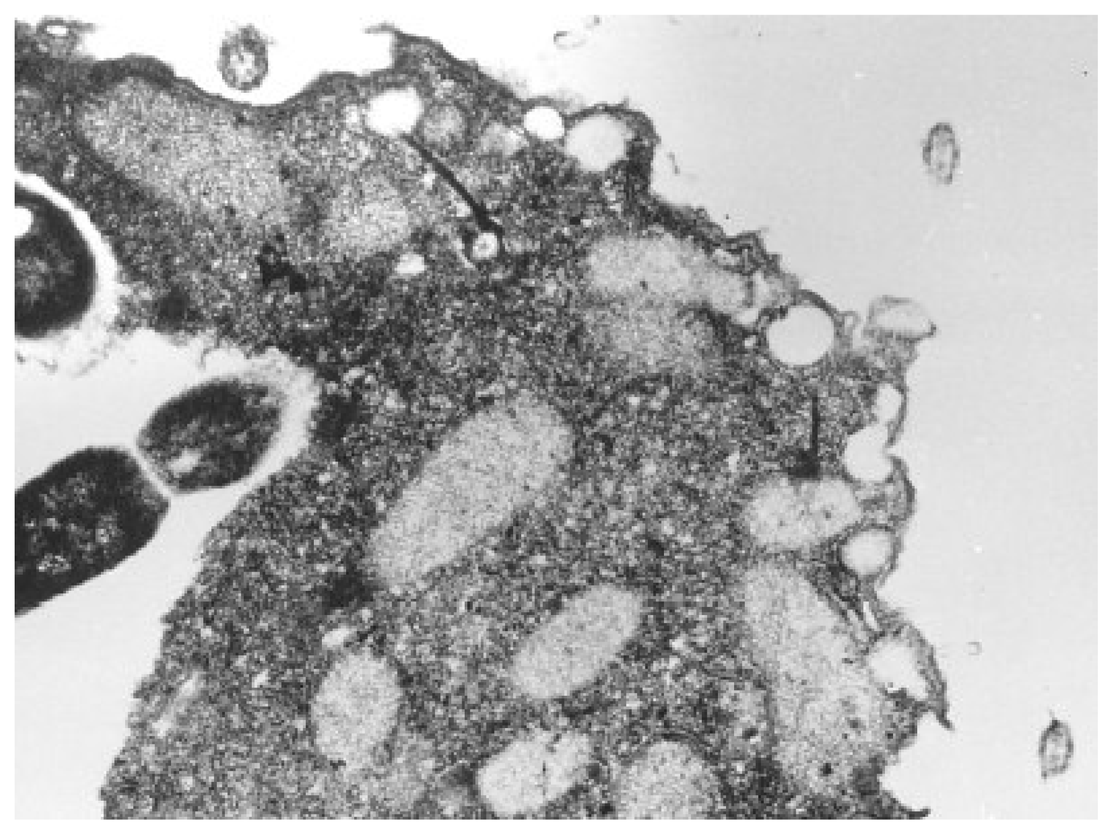
Nevertheless, most frequently studied unicellular organisms through QSAR toxicological analysis are from the Tetrahymena genus of ciliated protozoa. All species of the genus Tetrahymena are morphologically very similar; they display multiple nuclei: a diploid micronucleus found only in conjugating strains and a polyploid macronucleus present in all strains, which is the site of gene expression during vegetative growth, see Figure 3[82,83].

Tetrahymena species are very common in aquatic habitats and are non-pathogenic, have a short generation time and can be grown to high cell density in inexpensive media [81d]. As such, ecological, morphological, biochemical, and molecular features have been used over the years in attempts to classify them.

The earliest classifications were based on morphological and ecological data. At this level the presence or absence of a caudal cilium was regarded as an important character. Later, three morphological species complexes were distinguished: the pyriformis complex with smaller, bacterivorous species and less somatic kinetics; the rostrata complex with larger parasitic or histophagous species, more somatic kinetics, and the ability to form resting cysts; and the patula complex with species that undergo microstome-macrostome transformation. Within the complexes, particularly the pyriformis complex, species are distinguishable by their mating capacity and/or isozyme patterns. Finally, another approach based on the degree of parasitism was suggested. Since, the Tetrahymena species are free-living, as well as facultative and obligate parasites, it was suggested an evolutionary lineage from free-living species, considering Tetrahymena pyriformis to be the basal species, to facultative parasites, and then to obligate parasites [80,81a,82,84].

Accordingly, Tetrahymena pyriformis, a teardrop-shaped, unicellular, ciliated freshwater protozoan about 50 μm long, is found as the best candidate whose ecotoxicological activity is considered through the present S-SAR toward establishing a mechanistically coherent view of a certain class of xenobiotics on inter-correlated species.

3.3 Spectral-SAR Ecotoxicity of Tetrahymena pyriformis

Quite often, despite the tendency to submit a large class of descriptors to a QSAR analysis, this is not the best strategy [69], at least in ecotoxicology, and whenever a specific mode of action or the elucidation of the causal mechanistically scheme is envisaged.

More focused studies in ecotoxicology, and especially regarding T. pyriformis, have found that hydrophobicity (LogP) and electrophilicity (E_LUMO) phenomena plays a particular place in explaining the ecotoxicology of the species.

While hydrophobicity describes the penetration power of the xenobiotics though biological membranes, the other descriptors to be considered reflect the electronic and specific interaction between the ligand and target site of receptor.

Moreover, it was convincingly argued that the classical Hammett constant can be successfully rationalized by a pure structural index as the energy of the lowest unoccupied molecular orbital (LUMO) is [79]. These facts open the attractive perspective of considering the ecotoxicological studies through employing the Hansch-type structure-activity expansion:

$$A=b_0+b_1\left(\begin{array}{c}hydrophobic\\ descriptor\end{array}\right)+b_2\left(\begin{array}{c}electronic\\ descriptor\end{array}\right)+b_3\left(\begin{array}{c}steric\\ descriptor\end{array}\right),$$

(20)

thus also providing enough information from transport, electronic affinity and specific interaction at the molecular level, respectively.

However, in the present study, besides considering LogP as compulsory descriptor the molecular polarizability (POL) will be considered for modelling the electronic affinity for its inherent definition that implies the radius of the electrostatic sphere of electrostatic interaction. This way, the first stage of binding, through the radius of interaction, is accounted [85].

Then, the steric descriptor is chosen here, for simplicity, as the total molecular energy (E_TOT) in its ground state, for the reason that it is calculated at the optimum molecular geometry where the stereospecificity is included.

Under these circumstances the ecotoxic activity to Tetrahymena pyriformis, determined in a population growth impairment assay with a 40 h static design and population density measured spectrophotometrically as the endpoint A=Log (1/IGC₅₀) [86–90], from a series of xenobiotics of which majority are of phenol type is in

Table 3. The series of the xenobiotics of those toxic activities A= Log(1/IGC₅₀) were considered [86] along structural parameters LogP, POL (ų), and E_TOT (kcal/mol) as accounting for the hydrophobicity, electronic (polarizability) and steric (total energy at optimized 3D geometry) effects, respectively, derived with the help of HyperChem program [91].

No.	Compound		A	|1〉	Log P	POL	ETOT
	Name	Formulae	|Y〉	|X0〉	|X1〉	|X2〉	|X3〉
1	methanol	CH3OH	−2.67	1	−0.27	3.25	−11622.9
2	ethanol	C2H5OH	−1.99	1	0.08	5.08	−15215.4
3	butan-1-ol	C4H9OH	−1.43	1	0.94	8.75	−22402.8
4	butanone	C4H8O	−1.75	1	1.01	8.2	−21751.8
5	pentan-3-one	C5H10O	−1.46	1	1.64	10.04	−25344.6
6	phenol	C6H5OH	−0.21	1	1.76	11.07	−27003.1
7	aniline	C6H5NH2	−0.23	1	1.26	11.79	−24705.9
8	3-cresol	CH3-C6H4-OH	−0.06	1	2.23	12.91	−30597.6
9	4-methoxiphenol	OH-C6H4-O-CH3	−0.14	1	1.51	13.54	−37976.3
10	2-hydroxyaniline	OH-C6H4-NH2	0.94	1	0.98	12.42	−32095.4
11	Benzaldehyde	C6H5-CHO	−0.2	1	1.72	12.36	−29946.9
12	2-cresol	CH3-C6H4-OH	−0.27	1	2.23	12.91	−30597.2
13	3,4-dimeyhylphenol	C6H3(CH3)2OH	0.12	1	2.7	14.74	−34190.8
14	3-nitrotoluene	CH3-C6H4-NO2	0.05	1	0.94	13.98	−42365.1
15	4-chlorophenol	C6H5-O-Cl	0.55	1	2.28	13	−35307.6
16	2,4-dinitroaniline	C6H3(NO2)NH2	0.53	1	−1.75	15.22	−63030.2
17	2-methyl-1-4-naphtoquinone	C11H8O2	1.54	1	2.39	20.99	−49768.3
18	1,2-dichlorobenzene	C6H4Cl2	0.53	1	3.08	14.29	−36217.2
19	2,4-dinitrophenol	C6H3(NO2)OH	1.08	1	1.67	14.5	−65318
20	1,4-dinitrobenzene	C6H4N2O4	1.3	1	1.95	13.86	−57926.7
21	2,4-dinitrotoluene	C7H6(NO2)2	0.87	1	2.42	15.7	−61520.7
22	2,6-ditertbutil 4-methyl phenol	C15H23OH	1.8	1	5.48	27.59	−59316.5
23	2,3,5,6-tetrachloroaniline	C6H3NCl4	1.76	1	3.34	19.5	−57920.2
24	penthaclorophenol	C6Cl5OH	2.05	1	−0.54	20.71	−68512.4
25	phenylazophenol	C12H10N2O	1.66	1	4.06	22.79	−55488.9
26	pentabromophenol	C6Br5OH	2.66	1	5.72	24.2	−66151.5

considered.

It is worth mentioning that the number of compounds is in relevant ratio with the number of descriptors used, according with above Topliss-Costello rule, and that both chemical variability and congenericity are fulfilled since most of them reflect the phenolic toxicity.

The standard QSAR analysis of data of Table 3 for all possible models of actions reveals the multivariate equations displayed in

Table 4. QSAR equations through standard multi-linear routine of Satistica package [92] for all possible correlation models considered from data of Table 3.

Model	Variables	QSAR Equation	r	s	F
Ia	logP	$A^{Ia}=-0.547836+0.435669logP$	0.539	1.15	9.834
Ib	POL	$A^{Ib}=-2.84021+0.2166POL$	0.908	0.574	112.15
Ic	ETOT	$A^{Ic}=-2.50233-0.00007\hspace{0.17em}{E}_{TOT}$	0.882	0.644	84.015
IIa	logP, POL	$A^{IIa}=-2.91377-0.08109logP+0.23233POL$	0.911	0.58	55.930
IIb	logP, ETOT	$A^{IIb}=-2.64602+0.22991logP-0.00006\hspace{0.17em}{E}_{TOT}$	0.922	0.54	65.339
IIc	POL, ETOT	$A^{IIc}=-2.98407+0.13427POL-0.00003\hspace{0.17em}{E}_{TOT}$	0.939	0.478	86.503
III	logP, POL, ETOT	$A^{III}=-2.94395+0.06335logP+0.11206POL-0.00004E_{TOT}$	0.941	0.48	56.598

, together with their associate statistics:

$$r=\sqrt{1-\frac{SR}{SQ}},$$

(21)

$$s=\sqrt{\frac{SR}{N-M-1}}$$

(22)

$$F_{M{,}_{N-M-1}}=\frac{N-M-1}{M}\left(\frac{SQ}{SR}-1\right)$$

(23)

as correlation factor, standard error of estimate and Fisher index, respectively, in terms of the total number of residues, measuring the spreading of the input activities with respect to their estimated counterparts,

$$SR=\sum _{i=1}^N{\left(A_i-A_i^{PREDICTED}\right)}^2$$

(24)

and the total sum of squares,

$$SQ=\sum _{i=1}^N{\left(A_i-\overline{A}\right)}^2,$$

(25)

measuring the dispersion of the measured activities around their average:

$$\overline{A}=\frac{1}{N}\sum _{i=1}^N{A}_i.$$

(26)

while the number of compounds and descriptors were fixed to N = 26 and M = 3, in each endpoint case, respectively.

Before attempting a mechanistic analysis of the results, let us apply the S-SAR techniques to the same data of Table 3 by using the key (or spectral) equation-type (17) with the associated determinant completed with orthogonal and spectral coefficients of Eqs. (12) and (15), in each considered model of ecotoxic action, respectively.

More explicitly, in equations (27)–(29), the spectral equations are presented with their determinant forms that once expanded produce the spectral multi-linear dependencies of

Table 5. Spectral structure activity relationships (S-SAR) through determinants of Equations (27)–(29) for all possible correlation models considered from the data in Table 3.

Models	Vectors	S-SAR Equation
Ia	|X0〉, |X1〉	${\mid Y\rangle }^{Ia}=-0.547836\mid X_0\rangle +0.435669\mid X_1\rangle$
Ib	|X0〉, |X2〉	${\mid Y\rangle }^{Ib}=-2.84021\mid X_0\rangle +0.216598\mid X_2\rangle$
Ic	|X0〉, |X3〉	${\mid Y\rangle }^{Ic}=-2.50233\mid X_0\rangle -0.000067863\mid X_3\rangle$
IIa	|X0〉, |X1〉, |X2〉	${\mid Y\rangle }^{IIa}=-2.91377\mid X_0\rangle -0.0810929\mid X_1\rangle +0.232325\mid X_2\rangle$
IIb	|X0〉, |X1〉, |X3〉	${\mid Y\rangle }^{IIb}=-2.64602\mid X_0\rangle +0.229913\mid X_1\rangle -0.0000608117\mid X_3\rangle$
IIc	|X0〉, |X2〉, |X3〉	${\mid Y\rangle }^{IIc}=-2.98407\mid X_0\rangle +0.134274\mid X_2\rangle -0.0000324573\mid X_3\rangle$
III	|X0〉, |X1〉, |X2〉, |X3〉	${\mid Y\rangle }^{III}=-2.94395\mid X_0\rangle +0.0633549\mid X_1\rangle -0.112056\mid X_2\rangle -0.0000363728\mid X_3\rangle$

.

$$(\mathit{Ia}):|\begin{array}{ccc}{\mid Y\rangle }^{Ia}& 0.270385& 0.435669\\ \mid X_0\rangle & 1& 0\\ \mid X_1\rangle & 1.87808& 1\end{array}\mid =0\hspace{0.17em}\text{or}\mid \begin{array}{ccc}{\mid Y\rangle }^{Ia}& 0.268751& -0.547836\\ \mid X_1\rangle & 1& 0\\ \mid X_0\rangle & 0.304687& 1\end{array}|=0,$$

(27a)

$$(\mathit{Ib}):|\begin{array}{ccc}{\mid Y\rangle }^{Ib}& 0.270385& 0.216598\\ \mid X_0\rangle & 1& 0\\ \mid X_2\rangle & 14.3612& 1\end{array}\mid =0\hspace{0.17em}\text{or}\mid \begin{array}{ccc}{\mid Y\rangle }^{Ib}& 0.0441181& -2.84021\\ \mid X_2\rangle & 1& 0\\ \mid X_0\rangle & 0.0607278& 1\end{array}|=0,$$

(27b)

$$(\mathit{Ic}):|\begin{array}{ccc}{\mid Y\rangle }^{Ic}& 0.270385& 0.000067863\\ \mid X_0\rangle & 1& 0\\ \mid X_3\rangle & -40857.5& 1\end{array}\mid =0\hspace{0.17em}\text{or}\mid \begin{array}{ccc}{\mid Y\rangle }^{Ic}& 0.0000157064& -2.50233\\ \mid X_3\rangle & 1& 0\\ \mid X_0\rangle & -0.0000208433& 1\end{array}|=0,$$

(27c)

$$(\mathit{IIa}):\left|\begin{array}{cccc}{\mid Y\rangle }^{IIa}& 0.270385& 0.435669& 0.232325\\ \mid X_0\rangle & 1& 0& 0\\ \mid X_1\rangle & 1.87808& 1& 0\\ \mid X_2\rangle & 14.3612& 2.22431& 1\end{array}\right|=0,$$

(28a)

$$(\mathit{IIb}):\left|\begin{array}{cccc}{\mid Y\rangle }^{IIb}& 0.270385& 0.435669& -0.0000608117\\ \mid X_0\rangle & 1& 0& 0\\ \mid X_1\rangle & 1.87808& 1& 0\\ \mid X_3\rangle & -40857.5& -3383.5& 1\end{array}\right|=0,$$

(28b)

$$(\mathit{IIc}):\left|\begin{array}{cccc}{\mid Y\rangle }^{IIc}& 0.270385& 0.216598& -0.0000324573\\ \mid X_0\rangle & 1& 0& 0\\ \mid X_2\rangle & 14.3612& 1& 0\\ \mid X_3\rangle & -40857.5& -2536.37& 1\end{array}\right|=0,$$

(28c)

$$(\mathit{III}):\left|\begin{array}{ccccc}{\mid Y\rangle }^{III}& 0.270385& 0.435669& 0.232325& -0.0000363728\\ \mid X_0\rangle & 1& 0& 0& 0\\ \mid X_1\rangle & 1.87808& 1& 0& 0\\ \mid X_2\rangle & 14.3612& 2.22431& 1& 0\\ \mid X_3\rangle & -40857.5& -3383.5& -3306.57& 1\end{array}\right|=0.$$

(29)

Remarkably, one may easily note the striking similitude of the equations in Tables 4 and 5, respectively. Moreover, in equations (27) the spectral determinant was written in both possible ways of orthogonalization, nevertheless leading to the same results in Table 5. That is the computational proof that Spectral-SAR indeed provides a viable alternative to standard QSAR at each level of modelling, being independent of number of descriptors, compounds, or order of orthogonalization. We advocate on the computational advantage of S-SAR though lesser steps of computation and by the full analyticity of the delivered structure-activity equation, through a simple transparent determinant.

However, conceptually, S-SAR achieves a degree of novelty with respect to normal QSAR though that the spectral equation is given in terms of vectors rather than variables. Such features marks a fundamental achievements since this way we can deal at once with whole available data (of activity and descriptors) within a generalized vectorial space. Consequently, we may also use the spectral norm of the activity,

$$\Vert {\mid Y\rangle }^{MEASURED/PREDICTED}\Vert =\sqrt{\sum _{i=1}^n{(y_i^2)}^{MEASURED/PREDICTED}},$$

(30)

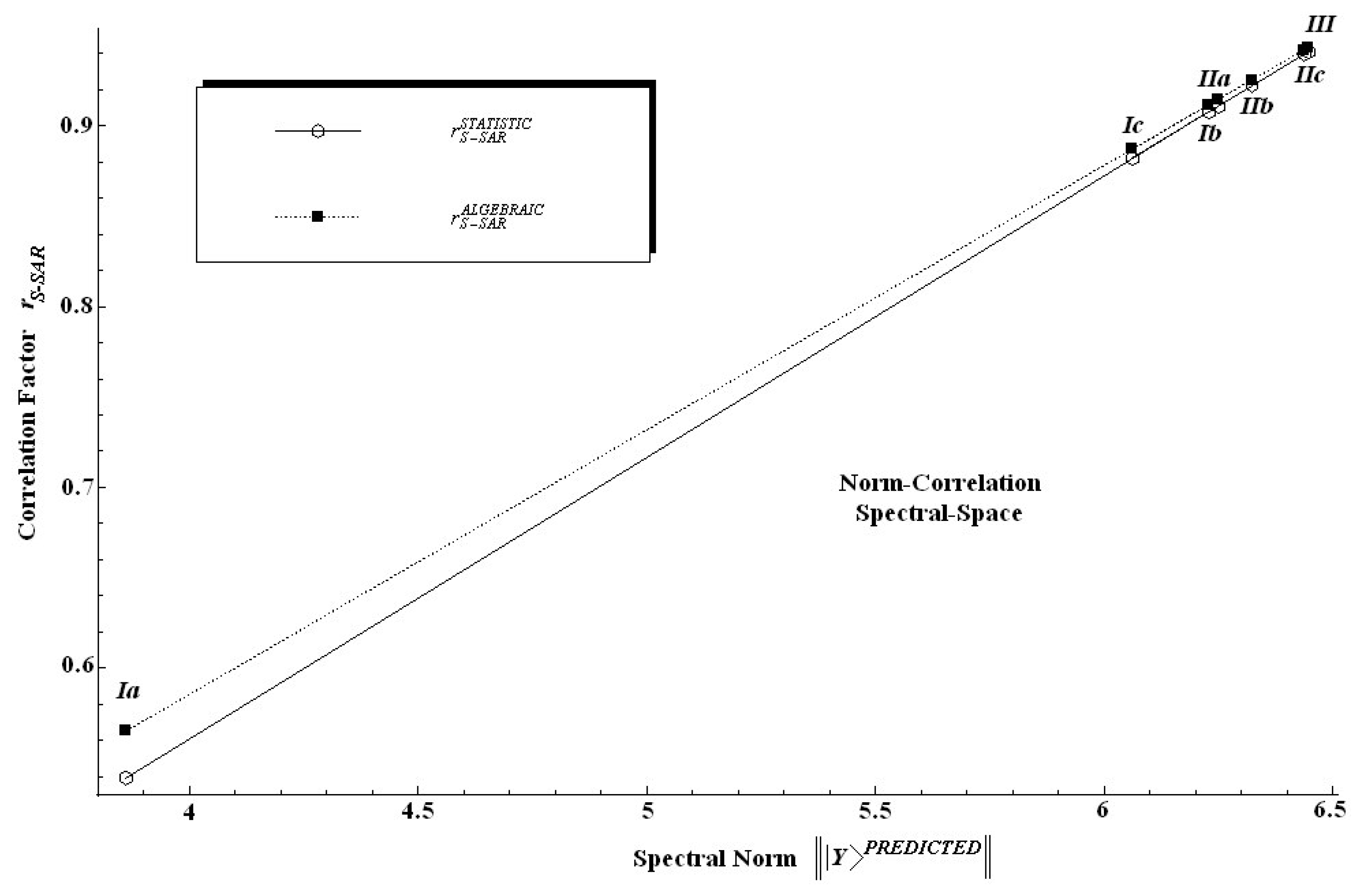
as the general tool by means which various models can be compared no matter of which dimensionality and of which multi-linear degree since they all reduce to a single number. This could help fulfill QSAR's old dream of providing a conceptual basis for the comparison of various models and end points by becoming a true science. Even more, while also accurately reproducing the statistics of the standard QSAR, the actual S-SAR permits the introduction of an alternative way of computing correlation factors by using the above spectral norm concept. As such the so called algebraic S-SAR correlation factor is defined as the ratio of the spectral norm of the predicted activity versus that of the measured one:

$$r_{S-SAR}^{ALGEBRAIC}=\frac{\Vert {\mid Y\rangle }^{PREDICTED}\Vert }{\Vert {\mid Y\rangle }^{MEASURED}\Vert },$$

(31)

Applying Eq. (31) to the present case of the measured spectral norm of T. pyriformis activity |||Y〉^MEASURED|| = 6.83243 the algebraic S-SAR correlation factors for the actual predicted models are given in

Table 6. The predicted spectral norm, the statistic and the algebraic correlation factors of the S-SAR models of Table 5, computed upon the general Eqs. (30), (21), and (31) since the entry data of Table 3 are employed, respectively.

	Ia	Ib	Ic	IIa	IIb	IIc	III
|||Y〉PREDICTED||	3.86176	6.22803	6.0607	6.24858	6.32297	6.43641	6.44557
$r_{S-SAR}^{STATISTIC}$	0.53905	0.90759	0.88193	0.91074	0.92214	0.9395	0.9409
$r_{S-SAR}^{ALGEBRAIC}$	0.56521	0.91154	0.88705	0.91455	0.92543	0.94204	0.94338

along the individual spectral norm of activity and the standard statistical correlation factor values.

The findings in Table 6 are twice relevant: first, because it is clear that the spectral norm parallels the statistic correlation factor; second, because, since the introduced algebraic correlation factor does the same job, it poses slightly higher values on a systematic basis.

In other words, one can say that in an algebraic sense the S-SAR furnishes systematically higher correlation factors than the standard QSAR does. This feature is also depicted in Figure 4 from where it is also noted that both correlation factors tend to approach each other near the ideal correlation factor, i.e. in the proximity of r = 1.00.

Nevertheless, we should note at this point that while a certain model does not satisfy the correlation factor criteria for being validated, i.e. r > 0.84, as is the case of the model (Ia) when only hydrophobicity is taken into account, this does not mean that the descriptor or chemical domain is less relevant; it is merely an indication that this descriptor may be further considered in a multivariate combination with others until produce better model.

Indeed, both within standard QSAR and S-SAR approaches all models except (Ia) are characterized by relevant statistics.

Next, aiming to see whether the obtained models can provide us a mechanistic model of chemical-biological interaction of tested xenobiotics on T. pyriformis species, the introduced spectral norm is employed in conjunction with algebraic or statistic correlation factors to compute the spectral paths between these models. Such an endeavor may lead to an intra-species analysis of models and form the first step for designing of integrated test batteries (or an expert system) at the inter-species level of ecotoxicology.

In this respect,

Table 7. Synopsis of the statistic and algebraic values of paths connecting the S-SAR models of Table 5 in the norm-correlation spectral-space of Figure 4.

Path	Value
	Statistic	Algebraic
Ia-IIa-III	2.61485	2.61132
Ia-IIb-III	2.61485	2.61132
Ia-IIc-III	2.61485	2.61132
Ib-IIa-III	0.220072	0.219855
Ib-IIb-III	0.220072	0.219855
Ib-IIc-III	0.220072	0.219855
Ic-IIa-III	0.389359	0.388969
Ic-IIb-III	0.389359	0.388969
Ic-IIc-III	0.389359	0.388969

presents the computed spectral distance between the models of the measured Log(1/IGC₅₀) endpoint of Table 3 though considering all path combinations that contain a single model for each class, with one and two descriptors, towards the closest model, i.e. (III), with respect to the ideal one. It follows that the paths are grouped according to the intermediary passing model while extreme models (initial and final) are kept fixed. Such ordered paths can be rationalized since a selection criterion is further introduced. Since paths are involved, one may learn from the well-established principle of nature according to which the events are linked by closest paths (in all classical and quantum spaces).

Therefore, we may formulate the S-SAR least path principle as follows: the hierarchy of models is driven by the minimum distance between endpoints (predicted norm of activities) of different classes of descriptors and of their combinations; whenever multiple minimum paths are possible, that principle applies iteratively downwards between individual intermediate models of paths, starting with that one with minimal spectral norm.

In our case, according to the enounced minimum spectral path rule, the diagram of Figure 5 is constructed. It emphasizes different mechanistic hierarchies of the T. pyriformis toxicophores. It comes out that, for instance, while three minimum paths result from Table 7, namely Ib-IIa-III, Ib-IIb-III, and Ib-IIc-III, only one is selected as giving the primary hierarchy, Ib-IIa-III, based on the fact that the spectral norm of IIa is the closest one to Ib. This is a purely mechanistic result since the correlation order in Table 6 would require that IIc be the next model chosen when starting from model Ib. At this point, we see that what is ordered from a statistical point of view may be degenerate in path length between the spectral norms. Therefore it appears that statistics might not be the most adequate criterion for SAR validity, since models with different correlations factors may be equally inter-related through spectral norms. Used exclusively, the statistic criteria will give little information about the subsidiary inter-species correlations in a unitary picture. On the contrary, the spectral path rule is able to formulate a scheme of connected paths between the models employing the natural principle of minimal action. Minimal action here means that minimal length between spectral norms of different categories of endpoints is more favorable and comes firstly into a process driven by the succession of activities. Thus, once the path Ib-IIa-III is naturally selected as the primary hierarchy of the ecotoxicity mechanism of T. pyriformis, one can expect that, in this interpretation of the minimum spectral paths, the envisioned sequence of actions towards the measured one can be causally modeled as the action of polarizability followed by that of hydrophobicity and finally by that of total energy, through the optimization of molecular geometry during the chemical-biological interactions involved. This picture tells that the covalent interaction is the most dominant one, in this case, and drives the approach between the xenobiotics and the cells of organism; then enters into action the transfer through cellular membrane and finally the stabilization being assured by the stereo-specificity of the compounds linked to the receptor site. This way, a molecular mechanism may be coherently formulated in terms of norms of actions and of their inter-distances.

Whenever the primary route is inhibited, the second hierarchy of action follows by excluding the models previously involved and based on the same least principle of action. The second initial model will be chose that which is nearest to the first one on the spectral norm scale. Then, from all equivalent paths the next step is made toward the closes neighbor in the spectral norm sense.

The second hierarchy results along the endpoints path Ic-IIb-III, see Figure 5. This tells us that, by some subsidiary, slower action, the stereo-specificity selection is the first stage of the chemical-biological interaction analyzed, followed by membrane transport and only then by the stabilization of chemical bonds through polarizability.

If the secondary route is somehow repressed, as well the third way of ecotoxicological action of T. pyriformis is also revealed as in Figure 5, Ia-IIc-III, again on the minimal activity action grounds constructed.

It is not surprising that the application of minimal action principles on the spectral activity norms furnished many, however ordered, ways in which chemical-biological interaction are present in nature. This is in accordance with the heuristically truth that the Nature reserves the privilege to develop many paths to achieve an action. The present S-SAR approach gives these new possibilities of hierarchically modelling of activities, in a way that the statistical analysis appears to be limited to single choices. Nevertheless, further work has to be performed by employing S-SAR method and of its minimal spectral path principle on many species and class of compounds in order to better validate the present results and algorithm.

4. Conclusions

Aiming to solve part of the many challenges posed by QSAR and its applications, with a view to generating a mechanistic-causal vision of the data recorded (measured or computed), the current paper introduces both a new analytical SAR modelling algorithm (the so-called Spectral-SAR method) and its associated minimum spectral action principle, following the activity norm of the models generated. As such, four possible branches of a QSAR expertise were identified, namely those based on the so called classical (of Hansch type), 3-dimensional (of CoMFA or MTD type), decisional (of genetic algorithm type) and orthogonal (of PCA type) – all proposing to furnish an appropriate analytical model for structure-chemical property or biological activity correlations. In this context the orthogonality problem was especially addressed, though the considered descriptors have to be as little collinear as possible in order to eliminate redundancies. Despite the fact that many QSAR approaches make use of algorithms that separate or transform initial non-orthogonal data into an orthogonal space, in search of a better correlation, many of them provide no significant improvement over the standard QSAR least square recipe. Instead, the present endeavor puts forth the orthogonal space (in Gram-Schmidt sense) only as an intermediate one in order to obtain from it the spectral expansion of concerned activity and descriptors like vectors in a high dimensional space. This way, through more algebraic transparent transformations the spectral structure-activity relationships (S-SAR) are formulated as viable alternative to the previous standard QSAR method. The actual S-SAR approach also provides the framework in which the spectral norm can be formulated as assigning a single number to any SAR problem with the meaning of encoded of all information of a model, including the statistics. However, the spectral norm permits the spectral formulation of the minimal action principle applicable among various tested models. As such, the ecotoxicology of the Tetrahymena pyriformis was studied in detail providing the hierarchical paths of molecular actions towards the recorded activity. Since all consecrated criteria of a valid SAR analysis to an ecotoxicology study were included, the present added principle, in terms of minimum path over spectral norms of possible models for a certain set of data, unfolds the perspective of a real mechanistic interpretation of the chemical-biological interaction based on QSAR equation. Nevertheless, further inter-species studies as well as the time-version of the least spectral norm principle have to be undertaken in order to better reveal the features and advantages of the present S-SAR method.

References

- Pogliani, L. Numbers Zero, One, Two, and Three in Science and Humanities. In Mathematical Chemistry Monographs; Volume 2, University of Kragujevac-Faculty of Science: Kragujevac, 2006. [Google Scholar]
- Putz, M.V. Systematic Formulation for Electronegativity and Hardness and Their Atomic Scales within Density Functional Softness Theory. Int. J. Quantum Chem 2006, 106, 361–386. [Google Scholar]
- Putz, M.V. Semiclassical Electronegativity and Chemical Hardness. J. Theor. Comp. Chem 2007, 6(1), 33–47. [Google Scholar]
- Delaney, J.S.; Mullaley, A.; Mullier, G.W.; Sexton, G.J.; Taylor, R.; Viner, R.C. Rapid construction of data tables for quantitative structure-activity relationship studies. J. Chem. Inf. Comput. Sci 1993, 33, 174–178. [Google Scholar]
- Klopman, G.; Balthasar, D.M.; Rosenkranz, H.S. Application of the computer-automated structure evaluation (CASE) program to the study of structure-biodegradation relationships of miscellaneous chemicals. Environ. Toxicol. Chem 1993, 12, 231–240. [Google Scholar]
- Basketter, D.; Dooms-Goossens, A.; Karlberg, A.-T.; Lepoittevin, J.P. The chemistry of contact allergy: why is a molecule allergenic? Contact Dermatitis 1995, 32, 65–73. [Google Scholar]
- Feijtel, T.C.J. Evaluation of the use of QSARs for priority settings and risk assessment. SAR and QSAR in Environmental Research 1995, 3, 237–245. [Google Scholar]
- Hermens, J.L.M.; Verhaar, H.J.M. QSARs in environmental toxicology and chemistry. ACS Symposium Series 1995, 606, 130–140. [Google Scholar]
- Hermes, J. Prediction of environmental toxicity based on structure-activity relationships using mechanistic information. Sci. Total Environ 1995, 171, 235–242. [Google Scholar]
- Hermens, J.; Balaz, S.; Damborsky, J.; Karcher, W.; Müller, M.; Peijnenburg, W.; Sabljic, A.; Sjöström, M. Assessment of QSARs for predicting fate and effects of chemicals in the environment: an international European project. SAR and QSAR in Environmental Research 1995, 3, 223–236. [Google Scholar]
- Ogihara, N. Drawing out drugs. Mod. Drug Discovery 2003, 6(9), 28–32. [Google Scholar]
- Hansch, C.; Hoekman, D.; Gao, H. Comparative QSAR: toward a deeper understanding of chemicobiological interactions. Chem. Rev 1996, 96, 1045–1075. [Google Scholar]
- Kubinyi, H.; Der Schlüssel zum Schloß, I. Grundlagen der Arzneimittelwirkung. Pharmazie in unserer Zeit 1994, 23 Jahrg. Nr.3. 158–168. [Google Scholar]
- Liwo, A.; Tarnowska, M.; Grzonka, Z.; Tempczyk, A. Modified Free-Wilson method for the analysis of biological activity data. Computers Chem 1992, 16, 1–9. [Google Scholar]
- Schmidli, H. Multivariate prediction for QSAR. Chemometrics and Intelligent Laboratory Systems 1997, 37, 125–134. [Google Scholar]
- Lhuguenot, J.C. Relation quantitative structure-activité (QSAR): une méthode mal reconnue car trop souvent mal utilisée. Ann. Fals. Exp. Chim 1995, 88, 293–310. [Google Scholar]
- Crippen, G.M.; Bradley, M.P.; Richardson, W.W. Why are binding-site models more complicated than molecules? Perspectives in Drug Discovery and Design 1993, 1, 321–328. [Google Scholar]
- Kier, L.B.; Hall, L.H. Molecular Connectivity in Structure-Activity Analysis; Research Studies Press: Letchworth, 1986. [Google Scholar]
- Balaban, A.T.; Motoc, I.; Bonchev, D.; Mekenyan, O. Topological indices for structure-activity correlations. Top. Curr. Chem 1983, 114, 21–55. [Google Scholar]
- Navia, M.A.; Peattie, D.A. Structure-based drug design: applications in immunopharmacology and immunosuppression. Immunology Today 1993, 14, 296–302. [Google Scholar]
- Perkins, T.D.J.; Dean, P.M. An exploration of a novel strategy for superposing several flexible molecules. J. Comput.-Aided Mol Design 1993, 7, 155–172. [Google Scholar]
- Lemmen, C.; Lengauer, T. Time-efficient flexible superposition of medium-sized molecules. J. Comput.-Aided Mol. Design 1997, 11, 357–368. [Google Scholar]
- Balaban, A.T.; Chiriac, A.; Motoc, I.; Simon, Z. Steric Fit in QSAR; Springer: Berlin; Lecture Notes in Chemistry Series; 1980. [Google Scholar]
- Simon, Z; Chiriac, A.; Holban, S.; Ciubotariu, D.; Mihalas, G. I. Minimum Steric Difference. The MTD Method for QSAR Studies; Res. Studies Press (Wiley): Letchworth, 1984. [Google Scholar]
- Duda-Seiman, C.; Duda-Seiman, D.; Dragoş, D.; Medeleanu, M.; Careja, V.; Putz, M.V.; Lacrămă, A.-M.; Chiriac, A.; Nuţiu, R.; Ciubotariu, D. Design of Anti-HIV Ligands by Means of Minimal Topological Difference (MTD) Method. Int. J. Mol. Sci 2006, 7, 537–555. [Google Scholar]
- Cramer, R.D.III; Patterson, D.E.; Bunce, J.D. Comparative molecular field analysis (CoMFA). 1. Effect shape on binding of steroids to carrier proteins. J. Am. Chem. Soc 1988, 110, 5959–5967. [Google Scholar]
- Cramer, R.D., III; DePriest, S.A.; Patterson, D.E.; Hecht, P. The developing practice of comparative molecular field analysis. In 3D QSAR in Drug Design. Theory, Methods and Applications; Kubinyi, H., Ed.; Escom: Leiden, 1993; pp. 443–485. [Google Scholar]
- Sun, J.; Chen, H.F.; Xia, H.R.; Yao, J.H.; Fan, B.T. Comparative study of factor Xa inhibitors using molecular docking/SVM/HQSAR/3D-QSAR methods. QSAR Comb. Sci 2006, 25, 25–45. [Google Scholar]
- Randić, M.; Jerman-Blazić, B.; Trinajstić, N. Development of 3-dimensional molecular descriptors. Comput. Chem 1990, 14, 237–246. [Google Scholar]
- Randić, M.; Razinger, M. Molecular topographic indices. J. Chem. Inf. Comput. Sci 1995, 35, 140–147. [Google Scholar]
- Manallack, D.T.; Livingstone, D.J. Artificial neural networks: application and chance effects for QSAR data analysis. Med. Chem. Res 1992, 2, 181–190. [Google Scholar]
- Manallack, D.T.; Livingstone, D.J. Limitations of functional-link nets as applied to QSAR data analysis. Quant. Struct-Act. Relat 1994, 13, 18–21. [Google Scholar]
- Marchant, C.A.; Combes, R.D. Artificial intelligence: the use of computer methods in the prediction of metabolism and toxicity. In Bioactive Compound Design: Possibilities for Industrial Use; Ford, M.G., Greenwood, R., Eds.; G.T. Brooks and R. Franke BIOS Scientific Publishers Limited, 1996. [Google Scholar]
- Moriguchi, I.; Hirono, S.; Matsushita, Y.; Liu, Q.; Nakagome, I. Fuzzy adaptive least squares applied to structure-activity and structure-toxicity correlations. Chem. Pharm. Bull 1992, 40, 930–934. [Google Scholar]
- Moriguchi, I.; Hirono, S. Fuzzy adaptive least squares and its use in quantitative structure-activity relationships. In QSAR and Drug Design – New Developments and Applications; Fujita, T., Ed.; Elsevier Science B. V, 1995. [Google Scholar]
- Vapnik, V.N. Statistical Learning Theory; John Wiley & Sons: New York, 1998. [Google Scholar]
- Vapnik, V.N. Estimation of Dependencies Based on Empirical Data; Springer-Verlag, Berlin, 1982. [Google Scholar]
- Schölkpof, B.; Burges, C.J.C.; Smola, A.J. (Eds.) Advances in Kernel Methods. Support Vector Learning; MIT Press: Cambridge, MA, 1999.
- Schölkpof, B.; Smola, A.J. Learning with Kernels; MIT Press: Cambridge, MA, 2002. [Google Scholar]
- Mangasarian, O.L.; Musicant, D.R. Succesive overrelaxation for support vector machines. IEEE Trans. Neural Networks 1999, 10, 1032–1036. [Google Scholar]
- Mattera, D.; Palmieri, F.; Haykin, S. Simple and robust methods for support vector expansions. IEEE Trans. Neural Networks 1999, 10, 1038–1047. [Google Scholar]
- Luan, F.; Ma, W.P.; Zhang, X.Y.; Zhang, H.X.; Liu, M.C.; Hu, Z.D.; Fan, B.T. QSAR study of polychlorinated dibenzodioxins, dibenzofurans, and biphenyls using the Heuristic method and support vector machine. QSAR Comb. Sci 2006, 25, 46–55. [Google Scholar]
- Sutter, J.M.; Kalivas, J.H.; Lang, P.K. Which principal components to utilize for principal component regression. J. Chemometrics 1992, 6, 217–225. [Google Scholar]
- Nendza, M.; Wenzel, A. Statistical approach to chemicals classification. Sci. Total Environ 1993, Supplement, 1459–1470. [Google Scholar]
- Cash, G.G.; Breen, J.J. Principal component analysis and spatial correlation: environmental analytical software tools. Chemosphere 1992, 24, 1607–1623. [Google Scholar]
- Hemmateenejad, B.; Miri, R.; Jafarpour, M.; Tabarzad, M.; Foroumadi, A. Multiple linear regression and principal component analysis-based prediction of the anti-tuberculosis activity of some 2-aryl-1,3,4-thiadiazole derivatives. QSAR Comb. Sci 2006, 25, 56–66. [Google Scholar]
- Randić, M. Resolution of ambiguities in structure-property studies by use of orthogonal descriptors. J. Chem. Inf. Comput. Sci 1991, 31, 311–320. [Google Scholar]
- Randić, M. Orthogonal Molecular Descriptors. New J. Chem 1991, 15, 517–525. [Google Scholar]
- Amić, D.; Davidović-Amić, D.; Trinajstić, N. Calculation of retention times of anthocyanins with orthogonalized topological indices. J. Chem. Inf. Comput. Sci 1995, 35, 136–139. [Google Scholar]
- Lučić, B.; Nikolić, S.; Trinajstić, N.; Juretić, D. The structure-property models can be improved using the orthogonalized descriptors. J. Chem. Inf. Comput. Sci 1995, 35, 532–538. [Google Scholar]
- Lučić, B.; Nikolić, S.; Trinajstić, N.; Jurić, A.; Mihalić, Z. A Structure-Property Study of the Solubility of Aliphatic Alcohols in Water. Croatica Chem. Acta 1995, 68, 417–434. [Google Scholar]
- Lučić, B.; Nikolić, S.; Trinajstić, N.; Juretić, D.; Jurić, A. A Novel QSPR Approach to Physicochemical Properties of the α-Amino Acids. Croatica Chem. Acta 1995, 68, 435–450. [Google Scholar]
- Šoškić, M.; Plavšić, D.; Trinajstić, N. Link between orthogonal and standard multiple linear regression models. J. Chem. Inf. Comput. Sci 1996, 36, 829–832. [Google Scholar]
- Klein, D.J.; Randić, M.; Babić, D.; Lučić, B.; Nikolić, S.; Trinajstić, N. Hierarchical orthogonalization of descriptors. Int. J. Quantum Chem 1997, 63, 215–222. [Google Scholar]
- Ivanciuc, O.; Taraviras, S.L.; Cabrol-Bass, D. Quasi-orthogonal basis sets of molecular graph descriptors as chemical diversity measure. J. Chem. Inf. Comput. Sci 2000, 40, 126–134. [Google Scholar]
- Putz, M.V. A Spectral Approach of the Molecular Structure – Biological Activity Relationship Part I. The General Algorithm. Annals of West University of Timişoara, Series of Chemistry 2006, 15, 159–166. [Google Scholar]
- Putz, M.V.; Lacrămă, A.M. A Spectral Approach of the Molecular Structure – Biological Activity Relationship Part II. The Enzymatic Activity. Annals of West University of Timişoara, Series of Chemistry 2006, 15, 167–176. [Google Scholar]
- Danko, P.E.; Popov, A.G.; Kozhevnikova, T.Y.A. Higher Mathematics in Problems and Exercises; Mir Publishers: Moscow; Volume I, 1983. [Google Scholar]
- Carnahan, B.; Luther, H.A.; Wilkes, J. Applied Numerical Methods; John Wiley & Sons: New York, 1969. [Google Scholar]
- Young, D.; Gregory, R. A Survey of Numerical Mathematics; Volume I, II, Addison-Wesley: Massachusets, 1973. [Google Scholar]
- Fadeeva, V. N. Computational Methods of Linear Algebra; Dover Publications: New York, 1959. [Google Scholar]
- Daudel, R.; Leroy, G.; Peeters, D.; Sana, M. Quantum Chemistry; John Wiley & Sons: New York, 1983. [Google Scholar]
- European Commission, Proposal for a Regulation of the European Parliament and of the Council concerning the Registration, Evaluation, Authorization and Restriction of chemicals (REACH), establishing a European Chemicals Agency and amending directive 1999/45/EC and Regulations (EC) {on Persistent Organic Pollutants}; Brussels, Belgium, 2003.
- OECD, Environment Directorate Joint Meetings of the Chemicals Committee and the Working Party on Chemicals, pesticides and Biotechnology. OECD Series on Testing and Assessment. Number 49. The report from Expert Group on (Quantitative) Structure-Activity Relationships [(Q)SAR] on the principles for the Validation of (Q)SARs; Paris, France, 2004.
- U.S. Environmental Protection Agency, ECOSAR: A computer program for estimating the ecotoxicity of industrial chemicals based on structure activity relationships. In EPA 748-R-002; National Center for Environmental Publications and Information: Cincinnati, OH, 1994; p. 34.
- US EPA AQUIRE (AQUatic toxicity Information REtrival). U.S. Environmental Protection Agency, 2002. ECOTOX User Guide: ECOTOXicology Database System. 2002. Version 3.0 [ http:www.epa.gov/ecotox/].
- Greim, H.; Csanády, G.; Filser, J. G.; Kreuzer, P.; Schwarz, L.; Wolff, T.; Werner, S. Biomarkers as tools in human health risk assessment. Clin. Chem 1995, 41, 1804–1808. [Google Scholar]
- Pangrekar, J.; Klopman, G.; Rosenkranz, H. S. Expert-system comparison of structural determinants of chemical toxicity to environmental bacteria. Environ. Toxicol. Chem 1994, 13, 979–1001. [Google Scholar]
- Klopman, G.; Zhang, Z.; Woodgate, S. D.; Rosenkranz, H. S. The structure-toxicity relationship challenge at hazardous waste sites. Chemosphere 1995, 31, 2511–2519. [Google Scholar]
- Judson, P. N. QSAR and expert systems in the prediction of biological activity. Pestic. Sci 1992, 36, 155–160. [Google Scholar]
- Hulzebos, E.; Posthumus, R. (Q)SAR: gatekeepers against risk on chemicals? SAR and QSAR in Environmental Research 2003, 14, 285–316. [Google Scholar]
- Hulzebos, E.; Sijm, D.; Traas, T.; Posthumus, R.; Maslankiewicz, L. Validity and validation of expert (Q)SAR systems. SAR and QSAR in Environmental Research 2005, 16, 385–401. [Google Scholar]
- Pavan, M.; Netzeva, T. I.; Worth, A. P. Validation of a QSAR model for acute toxicity. SAR and QSAR in Environmental Research 2006, 17, 147–171. [Google Scholar]
- Cronin, M. T. D.; Dearden, J. C. QSAR in toxicology. 1. Prediction of aquatic toxicity. Quant. Struct.-Act. Relat 1995, 14, 1–7. [Google Scholar]
- Cronin, M. T. D.; Dearden, J. C. QSAR in toxicology. 2. Prediction of acute mammalian toxicity and interspecies correlations. Quant. Struct.-Act. Relat 1995, 14, 117–120. [Google Scholar]
- Cronin, M. T. D.; Dearden, J. C. QSAR in toxicology. 3. Prediction of chronic toxicities. Quant. Struct.-Act. Relat 1995, 14, 329–334. [Google Scholar]
- Cronin, M. T. D.; Dearden, J. C. QSAR in toxicology. 4. Prediction of non-lethal mammalian toxicological endpoints, and expert systems for toxicity prediction. Quant. Struct.-Act. Relat 1995, 14, 518–523. [Google Scholar]
- Topliss, J. G.; Costello, J. D. Chance correlation in structure-activity studies using multiple regression analysis. J. Med. Chem 1972, 15, 1066–1069. [Google Scholar]
- Cronin, T.D.; Aptula, A.O.; Duffy, J.C.; Netzeva, T.I.; Rowe, P.H.; Valkova, I.V.; Wayne-Schultz, T. Comparative assessment of methods to develop QSARs for the prediction of the toxicity of phenols to Tetrahymena pyriformis. Chemosphere 2002, 49, 1201–1221. [Google Scholar]
- Lynn, D.H.; Small, E.B. Phylum Ciliophora. In Handbook of Protoctista; Margulis, L., Corliss, J.O., Melkonian, M., Chapman, D.J., Eds.; Jones and Bartlett Publishers: Boston, 1991. [Google Scholar]
- *** About systematic classification of Tetrahymena pyriformis:http://www.ucmp.berkeley.edu/protista/ciliata/ciliatamm.html accessed December 2006.http://www.ns.purchase.edu/biology/bio1560lab/protista.htm accessed December 2006.http://www.bch.umontreal.ca/ogmp/projects/tpyri/org.html accessed December 2006.http://www-micro.msb.le.ac.uk/video/Tetrahymena.html accessed December 2006.
- Niles, E.G.; Jain, R.K. Physical Map of the Ribosomal Ribonucleic Acid Gene from Tetrahymena pyriformis. Biochemistry 1981, 20, 905–909. [Google Scholar]
- Manasherob, R.; Ben-Dov, E.; Zaritsky, A.; Barak, Z. Germination, growth, and sporulation of Bacillus thuringiensis subsp. israelensis in excreted food vacuoles of the protozoan Tetrahymena pyriformis. Appl. Environ. Microbiol 1998, 64, 1750–1758. [Google Scholar]
- Strüder-Kypke, M.C.; Wright, A.-D.G.; Jerome, C.A.; Lynn, D.H. Parallel evolution of histophagy in ciliates of the genus Tetrahymena. BMC Evolutionary Biology 2001, 1, 5. [Google Scholar]
- Putz, M.V.; Russo, N.; Sicilia, E. Atomic Radii Scale and Related Size Properties from Density Functional Electronegativity Formulation. Journal of Physical Chemistry A 2003, 107, 5461–5465. [Google Scholar]
- Cronin, M.T.D.; Netzeva, T.I.; Dearden, J.C.; Edwards, R.; Worgan, A.D.P. Assessment and modeling of the toxicity of organic chemicals to Chlorella vulgaris: development of a novel database. Chem. Res. Toxicol 2004, 17, 545–554. [Google Scholar]
- Schultz, T.W. TETRATOX: the Tetrahymena pyriformis population growth impairment endpoints. A surrogate for fish lethality. Toxicol. Methods 1997, 7, 289–309. [Google Scholar]
- Schultz, T.W. Structure-toxicity Relationships for benzene evaluated with Tetrahymena pyriformis. Chem. Res. Toxicol 1999, 12, 1262–1267. [Google Scholar]
- Schultz, T.W.; Cronin, M.T.D.; Netzeva, T.I.; Aptula, A.O. Structure-toxicity relationships for aliphatic chemicals evaluated with Tetrahymena pyriformis. Chem. Res. Toxicol 2002, 15, 1602–1609. [Google Scholar]
- Schultz, T.W.; Netzeva, T.I.; Cronin, M.T.D. Selection of data sets for QSARs: analyses of Tetrahymena toxicity from aromatic compounds. SAR and QSAR in Environmental Research 2003, 14, 59–81. [Google Scholar]
- Hypercube, Inc, 2002; HyperChem 7.01 [Program package].
- StatSoft, Inc, 1995; STATISTICA for Windows [Computer program manual].
© 2007 by MDPI Reproduction is permitted for noncommercial purposes.
Share and Cite
MDPI and ACS Style
Putz, M.V.; Lacrămă, A.-M. Introducing Spectral Structure Activity Relationship (S-SAR) Analysis. Application to Ecotoxicology. Int. J. Mol. Sci. 2007, 8, 363-391. https://doi.org/10.3390/i8050363
AMA Style
Putz MV, Lacrămă A-M. Introducing Spectral Structure Activity Relationship (S-SAR) Analysis. Application to Ecotoxicology. International Journal of Molecular Sciences. 2007; 8(5):363-391. https://doi.org/10.3390/i8050363
Chicago/Turabian StylePutz, Mihai V., and Ana-Maria Lacrămă. 2007. "Introducing Spectral Structure Activity Relationship (S-SAR) Analysis. Application to Ecotoxicology" International Journal of Molecular Sciences 8, no. 5: 363-391. https://doi.org/10.3390/i8050363