Prediction of Human Intestinal Absorption by GA Feature Selection and Support Vector Machine Regression

Abstract
:
1. Introduction
2. Data Sets
3. Methods
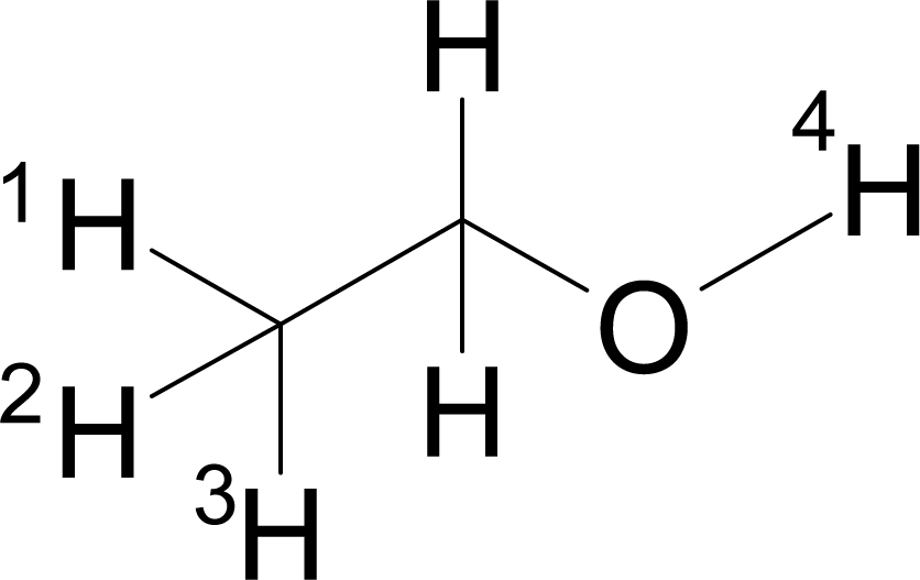
3.1. Descriptors
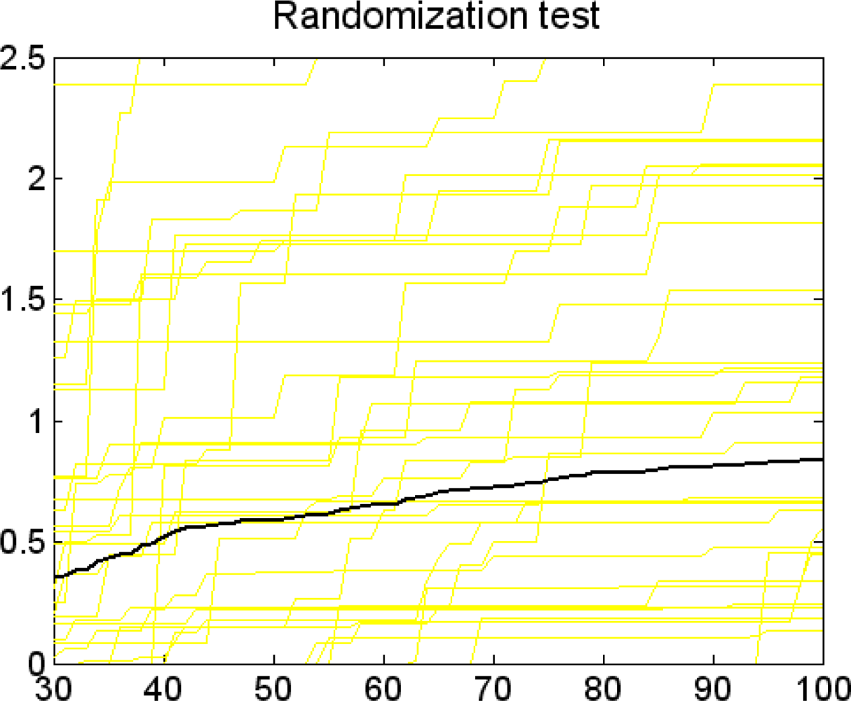
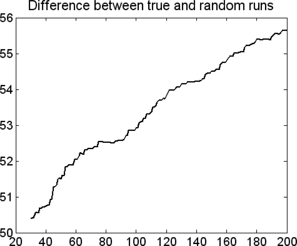
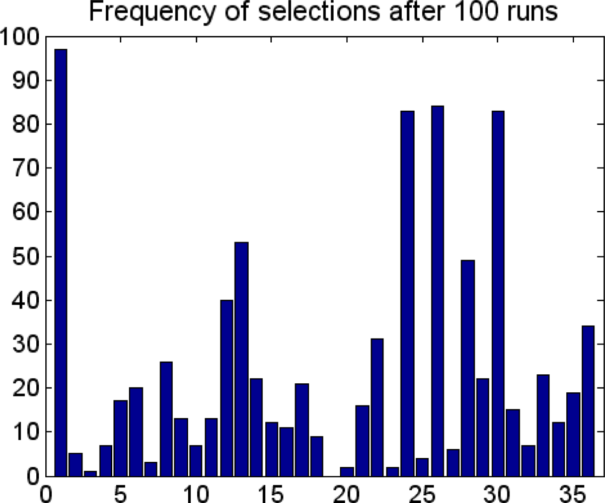
3.2. Feature Selection of the Descriptors with GA Strategy
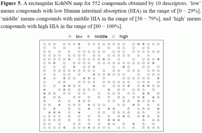
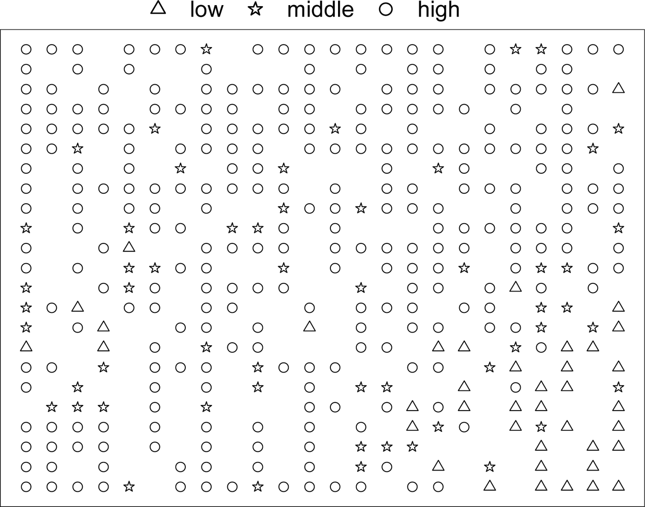
3.3. Training/Test Set Selection with Kohonen's Self-organizing Neural Network
3.4. Support Vector Machine (SVM) Analysis
4. Results and Discussion
4.1. Partial Least Square (PLS) Models
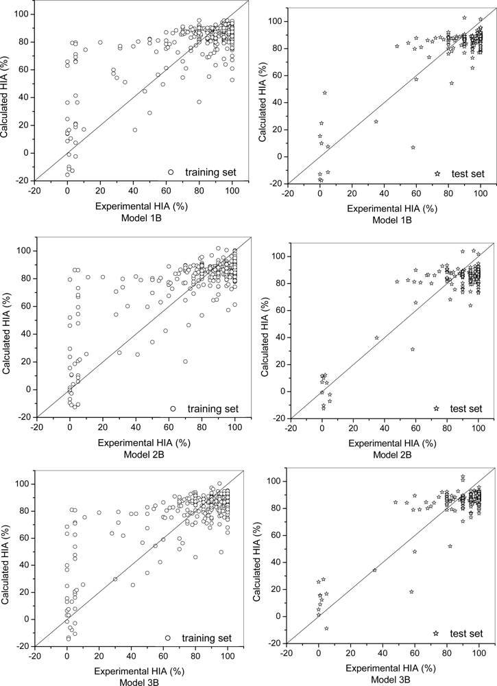
4.2. Support Vector Machine (SVM) Models
5. Conclusions
Acknowledgments
References and Notes
- Davis, AM; Riley, RJ. Predictive ADMET Studies, the Challenges and the Opportunities. Curr. Opin. Chem. Biol. 2004, 8, 378–386. [Google Scholar]
- Wessel, MD; Mente, S. ADME by Computer. Ann. Rep. Med. Chem 2001, 36, 257–266. [Google Scholar]
- Varma, MVS; Sateesh, K; Panchagnula, R. Functional Role of P-Glycoprotein in Limiting Intestinal Absorption of Drugs: Contribution of Passive Permeability to P-Glycoprotein Mediated Efflux Transport. Mol. Phamaceutics 2005, 2, 12–21. [Google Scholar]
- Xue, Y; Li, ZR; Yap, CW; Sun, LZ; Chen, X; Chen, YZ. Effect of Molecular Descriptor Feature Selection in Support Vector Machine Classification of Pharmacokinetic and Toxicological Properties of Chemical Agents. J. Chem. Inf. Comput. Sci 2004, 44, 1630–1638. [Google Scholar]
- Klopman, G; Stefan, LR; Saiakhov, RD. ADME Evaluation 2. A Computer Model for the Prediction of Intestinal Absorption in Humans. Euro. J. Pharm. Sci. 2002, 17, 253–263. [Google Scholar]
- Perez, MA; Sanz, MB; Torres, LR; Avalos, RG; Gonzalez, MP; Diaz, HG. A Topological Sub-structural Approach for Predicting Human Intestinal Absorption of Drugs. Eur. J. Med. Chem. 2004, 39, 905–916. [Google Scholar]
- Sun, HJ. A Universal Molecular Descriptor System for Prediction of LogP, LogS, LogBB, and Absorption. J. Chem. Inf. Comput. Sci. 2004, 44, 748–757. [Google Scholar]
- Wessel, MD; Jurs, PC; Tolan, JW; Muskal, SM. Prediction of Human Intestinal Absorption of Drug Compounds from Molecular Structure. J. Chem. Inf. Comput. Sci. 1998, 38, 726–735. [Google Scholar]
- Zhao, YH; Le, J; Abraham, MH; Hersey, A; Eddershaw, PJ; Luscombe, CN; Boutina, D; Beck, G; Sherborne, B; Cooper, I; Platts, JA. Evaluation of Human Intestinal Absorption Data and Subsequent Derivation of a Quantitative Structure-activity Relationship (QSAR) with the Abraham Descriptors. J. Pharm. Sci 2001, 90, 749–784. [Google Scholar]
- Abraham, MH; Zhao, YH; Le, J; Hersey, A; Luscombe, CN; Reynolds, DP; Beck, G; Sherborne, B; Cooper, I. On the Mechanism of Human Intestinal Absorption. Eur. J. Med. Chem 2002, 37, 595–605. [Google Scholar]
- Cruciani, G.; Pastor, M; Guba, W. A New Tool for the Pharmacokinetic Optimization of Lead Compounds. Euro. J. Pharm. Sci 2000, 2, S29–S39. [Google Scholar]
- Agatonovic-Kustrin, S; Beresford, R; Yusof, APM. Theoretically-derived Molecular Descriptors Important in Human Intestinal Absorption. J. Pharm. Biomed. Anal. 2001, 25, 227–237. [Google Scholar]
- Osterberg, T; Norinder, U. Prediction of Polar Surface Area and Drug Transport Processes Using Simple Parameters and PLS Statistics. Euro. J. Pharm. Sci. 2001, 12, 327–337. [Google Scholar]
- Norinder, U; Osterberg, T; Artursson, P. Theoretical Calculation and Prediction of Intestinal Absorption of Drugs in Humans Using MolSurf Parametrization and PLS Statistics. Euro. J. Pharm. Sci. 1999, 8, 49–56. [Google Scholar]
- Niwa, T. Using General Regression and Probabilistic Neural Networks to Predict Human Intestinal Absorption with Topological Descriptors Derived from Two-Dimensional Chemical Structures. J. Chem. Inf. Comput. Sci. 2003, 43, 113–119. [Google Scholar]
- Wegner, JK; Frohlich, H; Zell, A. Feature Selection for Descriptor Based Classification Models. 2. Human Intestinal Absorption (HIA). J. Chem. Inf. Comput. Sci. 2004, 44, 931–939. [Google Scholar]
- ADRIANA.
- Gasteiger, J. Of Molecules and Humans. J. Med. Chem. 2006, 49, 6429–6434. [Google Scholar]
- Cerius2 version 4.10L.
- .
- Zupan, J; Gasteiger, J. Neural Networks in Chemistry and Drug Design, 2 ed; Ed.; Wiley-VCH; : Weinheim; , 1999. [Google Scholar]
- Chang, CC; Lin, CJ. LIBSVM: A Library for Support Vector Machines, 2001.
- Hou, T; Wang, J; Zhang, W; Xu, X. ADME Evaluation in Drug Discovery. 7. Prediction of Oral Absorption by Correlation and Classification. J. Chem. Inf. Model 2007, 47, 208–218. [Google Scholar]
- .
- .
- .
- Ertl, P; Rohde, B; Selzer, P. Fast Calculation of Molecular Polar Surface Area as a Sum of Fragment-Based Contributions and its Application to the Prediction of Drug Transport Properties. J. Med. Chem. 2000, 43, 3714–3717. [Google Scholar]
- Yan, A; Gasteiger, J. Prediction of Aqueous Solubility of Organic Compounds Based on a 3D Structure Representation. J. Chem. Inf. Comput. Sci. 2003, 43, 429–434. [Google Scholar]
- Yan, A; Gasteiger, J; Krug, M; Anzali, S. Linear and Nonlinear Functions on Modeling the Aqueous Solubility of Organic Compounds by Two Structure Representation Methods. J. Comput.-Aided Mol. Design 2004, 18, 75–87. [Google Scholar]
- Wang, R; Gao, Y; Lai, L. Calculating Partition Coefficient by Atom-Additive Method. Perspect. Drug Discovery Des. 2000, 19, 47–66. [Google Scholar]
- Lipinski, CA; Lombardo, F; Dominy, BW; Feeney, PJ. Experimental and Computational Approaches to Estimate Solubility and Permeability in Drug Discovery and Development Settings. Adv. Drug. Deliv. Rev. 2001, 46, 3–26. [Google Scholar]
- Wagener, M; Sadowski, J; Gasteiger, J. Autocorrelation of Molecular Surface Properties for Modeling Corticosteroid Binding Globulin and Cytosolic Ah Receptor Activity by Neural Networks. J. Am. Chem. Soc. 1995, 117, 7769–7775. [Google Scholar]
- Gasteiger, J; Marsili, M. A New Method for Calculating Atomic Charges in Molecules. Tetrahedron Lett. 1978, 34, 3181–3184. [Google Scholar]
- Gasteiger, J; Marsili, M. Iterative Partial Equalization of Orbital Electronegativity - A Rapid Access to Atomic Charges. Tetrahedron 1980, 36, 3219–3228. [Google Scholar]
- Kleinoeder, T. Prediction of Properties of Organic Compounds; , Ph.D. thesis, University of Erlangen-Nuernberg, 2005.
- Gasteiger, J; Hutchings, MG. Quantitative Models of Gas-Phase Proton Transfer Reaction Involving Alcohols, Ethers and Their Thio Analogs. Correlation Analyses Based On Residual Electronegativity and Effective Polarizability. J. Am. Chem. Soc. 1984, 106, 6489–6495. [Google Scholar]
- .
- Leardi, R; Terrile, M. Genetic Algorithm as a Strategy for Feature Selection. J. Chemom. 1992, 6, 267–281. [Google Scholar]
- Leardi, R. Application of a Genetic Algorithm to Feature Selection under Full Validation Condition and to Outlier Detection. J. Chemom. 1994, 9, 65–79. [Google Scholar]
- Leardi, R. Application of Genetic Algorithm–PLS for Feature Selection in Spectral Data sets. J. Chemom. 2000, 14, 643–655. [Google Scholar]
- .
- Simon, V; Gasteiger, J; Zupan, J. A Combined Application of Two Different Neural Network Types for the Prediction of Chemical Reactivity. J. Am. Chem. Soc. 9148–9159.
- Yan, AX; Gasteiger, J. Prediction of Aqueous Solubility of Organic Compounds by Topological Descriptors, QSAR Comb. Sci. 2003, 22, 821–829. [Google Scholar]
- .
- .
- Toutios, A; Margaritis, K. Mapping between the Speech Signal and Articulatory Trajectories. In Proceedings of the 7th Hellenic European Conference on Computer Mathematics and Its Applications (HERCMA-2005); September 2005; Athens, Greece. [Google Scholar]


| Model 1A
| Model 2A
| Model 3A
| |||
|---|---|---|---|---|---|
| descriptors | coefficient | descriptors | coefficient | descriptors | coefficient |
| Nrule5 | 10.3161 | Nrule5 | −10.0335 | Nrule5 | 8.4014 |
| Hdon | 2.8231 | Nrot | 1.4978 | Nrot | 1.2908 |
| LogS | 2.9385 | LogP | 1.4458 | LogP | 1.4358 |
| MW | −0.0194 | Hdon | 2.7628 | Hdon | 2.5400 |
| TPSA | 0.1446 | Jurs- FNSA3 | 85.0957 | Jurs- FNSA3 | 97.3355 |
| Acorr_Sigchg_3 | 14.5617 | Jurs-RPCG | 38.3653 | Jurs-RPCG | 28.8753 |
| LogS | 1.7446 | ||||
| MW | −0.0236 | ||||
| Acorr_Sigchg_3
| 10.2598
| ||||
| Dc | 96.5824 | Dc | 102.393 | Dc | 105.466 |
| Model | Training set
| Test set
| RMS | |||||
|---|---|---|---|---|---|---|---|---|
| n | r | s | n | r | s | |||
| Model 1A | PLS | 380 | 0.72 | 15.10 | 172 | 0.83 | 13.06 | 18.79 |
| Model 1B | SVM | 380 | 0.79 | 13.25 | 172 | 0.87 | 10.98 | 16.68 |
| Model 2A | PLS | 380 | 0.73 | 14.67 | 172 | 0.83 | 13.12 | 18.67 |
| Model 2B | SVM | 380 | 0.80 | 13.40 | 172 | 0.89 | 9.72 | 16.35 |
| Model 3A | PLS | 380 | 0.74 | 14.97 | 172 | 0.83 | 13.36 | 18.18 |
| Model 3B | SVM | 380 | 0.81 | 12.50 | 172 | 0.88 | 9.14 | 16.00 |
| Hou’s model17 | 455 | 0.84 | 15.50 | 98 | 0.90 | - | - | |
© 2008 by MDPI This article is an open-access article distributed under the terms and conditions of the Creative Commons Attribution license (http://creativecommons.org/licenses/by/3.0/).
Share and Cite
Yan, A.; Wang, Z.; Cai, Z. Prediction of Human Intestinal Absorption by GA Feature Selection and Support Vector Machine Regression. Int. J. Mol. Sci. 2008, 9, 1961-1976. https://doi.org/10.3390/ijms9101961
Yan A, Wang Z, Cai Z. Prediction of Human Intestinal Absorption by GA Feature Selection and Support Vector Machine Regression. International Journal of Molecular Sciences. 2008; 9(10):1961-1976. https://doi.org/10.3390/ijms9101961
Chicago/Turabian StyleYan, Aixia, Zhi Wang, and Zongyuan Cai. 2008. "Prediction of Human Intestinal Absorption by GA Feature Selection and Support Vector Machine Regression" International Journal of Molecular Sciences 9, no. 10: 1961-1976. https://doi.org/10.3390/ijms9101961