Topological indices are a convenient method of translating chemical constitution into numerical values that can be used for correlations with physical, chemical or biological properties. This method has been introduced by Harold Wiener as a descriptor for explaining the boiling points of paraffins [1–3]. If d(u, v) is the distance of the vertices uand νof the undirected connected graph G (i.e., the number of edges in the shortest path that connects u and v) and V (G) is the vertex set of G, then the Wiener index of G is the half sum of distances over all its vertex pairs (u, v): W ( G ) = 1 2 ∑ u ∈ V ( G ) ∑ ν ∈ V ( G ) d ( u , ν ) .

A unified approach to the Wiener topological index and its various recent modifications is presented. Among these modifications particular attention is paid to the Hyper-Wiener, Harary, Szeged, Cluj and Schultz indices as well as their numerous variants and generalizations [4–10]. The Schultz index of the graph was introduced by Schultz [14] in 1989 and is defined as follows: S ( G ) = 1 2 ∑ u ∈ V ( G ) ∑ ν ∈ V ( G ) ( deg ( u ) + deg ( ν ) ) d ( u , ν ) ,where deg(u) is the degree of the vertex u.

The main chemical applications and mathematical properties of this index were established in a series of studies [12–15]. Also a comparative study of molecular descriptors showed that the Schultz index and Wiener index are mutually related [16–18].

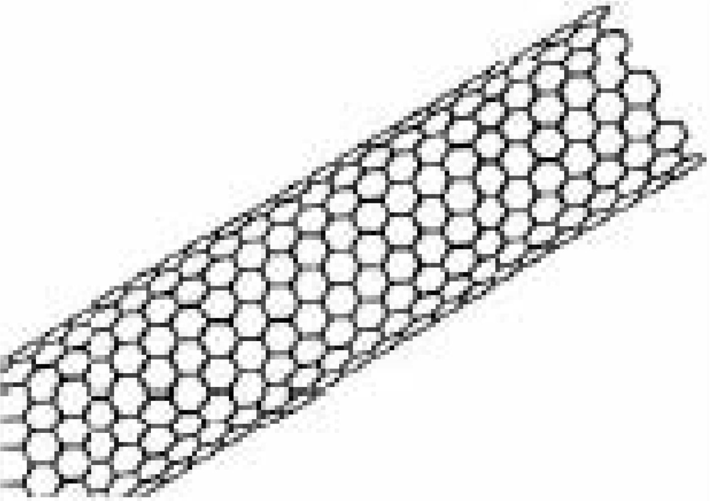
Carbon nanotubes, the one-dimensional carbon allotropes, are intensively studied with respect to their promise to exhibit unique physical properties: mechanical, optical electronic etc. [19–21]. In [19], Diudea et al. obtained the Wiener index of TUV C₆[2p; q], the armchair polyhex nanotube (see Figure 1). Here we find a relation between the Schultz index and Wiener index of this molecule. By using this relation we find an exact expression for the Schultz index of the same. The Appendix includes a Maple program [22] to produce the graph of TUV C₆[2p; q], and to compute the Schultz index of the graph.

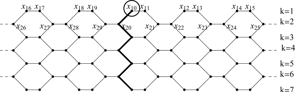
Throughout this paper G := TUV C₆[2p; q]denotes an arbitrary armchair polyhex nanotube in terms of its circumference 2p and their length q, see Figure 2. At first we consider an armchair lattice and choose a coordinate label for it, as illustrated in Figure 2. The distance of a vertex u of G is defined as d ( u ) = ∑ x ∈ V ( G ) d ( u , x ) ,the summation of distances between v and all vertices of G. By considering this notation the following lemma gives us a relation between the Schultz and Wiener index of G.

Lemma 1. For the graph G = TUV C₆[2p; q]we have S ( G ) = 6 W ( G ) - 2 ∑ u ∈ l e v e l   1 d ( u ) .

Proof: For each k such that 1 ≤ k ≤ q put A_k := {u ε V (G)│u; level k}( see Figure 2). Then S ( G )   = 1 2 ∑ u ∈ V ( G ) ∑ ν ∈ V ( G ) ( deg ( u ) + deg ( ν ) ) d ( u , ν )                         = 1 2 ∑ u ∈ V ( G ) ∑ ν ∈ V ( G ) deg ( u ) d ( u , ν ) + 1 2 ∑ u ∈ V ( G ) ∑ ν ∈ V ( G ) deg ( ν ) d ( u , ν )                       = 1 2 ∑ u ∈ V ( G ) ∑ ν ∈ V ( G ) deg ( u ) d ( u , ν ) + 1 2 ∑ ν ∈ V ( G ) ∑ u ∈ V ( G ) deg ( ν ) d ( u , ν )                       = 1 2 ∑ u ∈ V ( G ) deg ( u ) ∑ ν ∈ V ( G ) d ( u , ν ) + 1 2 ∑ ν ∈ V ( G ) deg ( ν ) ∑ u ∈ V ( G ) d ( u , ν )                       = 1 2 ∑ u ∈ V ( G ) deg ( u ) d ( u ) + 1 2 ∑ ν ∈ V ( G ) deg ( ν ) d ( ν )                     = ∑ u ∈ V ( G ) deg ( u ) d ( u )But deg ( u ) = { 2 if u ∈ A 1 ∪ A q 3 if o t h e r w i s e .

Also in the graph G it is clear that ∑ u ∈ A 1 d ( u ) = ∑ u ∈ A q d ( u ). Therefore S ( G ) = ∑ u ∈ V ( G ) deg ( u ) d ( u ) = ∑ u ∈ A 1 ∪ A q deg ( u ) d ( u ) + ∑ u ∈ V ( G ) \ ( A 1 ∪ A q ) d e g ( u ) d ( u )                       = ∑ u ∈ A 1 ∪ A q 2 d ( u ) + ∑ u ∈ V ( G ) \ ( A 1 ∪ A q ) 3 d ( u )                     = 3 ∑ u ∈ V ( G ) d ( u ) - 2 ∑ u ∈ A 1 d ( u )                   = 6 W ( G ) - 2 ∑ u ∈ A 1 d ( u ) .This completes the proof.

To compute the d(u) in the graph G, when u is a vertex in level 1, we first prove the following lemma.

Lemma 2.The sum of distances of one vertex of level 1 to all vertices of level k is given by w k : = ∑ x ∈ l e v e l   k d ( x 10 , x ) = ∑ x ∈   l e v e l   k d ( x 11 , x )                                                                                         ⋮                                                                                         = { 2 p 2 + k 2 - 2 k - 2 p + 1 + H ( p , k ) if 1 ≤ k < p p ( p + 2 k - 2 ) if k ≥ p ,where H ( p , k ) = { 2 p - 1 if k + p   is    even 2 p if k + p   is  odd .

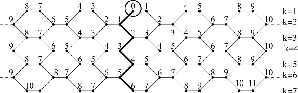
Proof:We calculate the value of w_k. We consider that the tube can be built up from two halves collapsing at the polygon line joining x₁₀ to x_q,0 (see Figure 2). The right part is the graph G₁ which consists of vertical polygon lines 0, 1,. . . . . p and x₁₀ is one of the vertices in the first row of the graph G₁. The left part is the graph G₂ which consists of vertical polygon lines (p + 1); (p + 2),. . . . , 2p –1. We change the indices of the vertices of G₂ in the following way: V ( G 2 ) = { x ^ j i | x ^ j , i = x j , 2 p - i ∈ V ( G ) }

(See Figure 3)

We must consider two cases:Case 1: If k ≥ p. In the graphs G1 and for 0 ≤ i < k we have d ( x 10 , x k , i ) = k + i - 1.

Also in the graphs G₂ and for 1 ≤.i < k we have d ( x 10 , x ^ k , i ) = k + i - 1.So ∑ x ∈   l e v e l   k d ( x 10 , x ) = 2 ∑ i = 1 p - 1 ( k + i - 1 ) + ( 0 + k - 1 ) + ( p + k - 1 ) = p ( p + 2 k - 2 ) .

Case 2: If k < p. First suppose that 1 ≤ i < k. In the graphs G₁ and G₂ we have d ( x 10 , x k , i ) = k + i - 1 = d ( x 10 , x ^ k , i ) = k + i - 1.

Now suppose that k ≤ i ≤ p. Then in the graph G₁ we can see that if k is odd, then d ( x 10 , x k , i ) = { 2 i if i   is even 2 i - 1 if i   is odd and if k is even, then d ( x 10 , x k , i ) = { 2 i - 1 if i   is even 2 i if i   is odd . Also in G₂ we have d ( x 10 , x ^ k , i ) = { 2 i if i   is even 2 i + 1 if i   is odd if k is odd d ( x 10 , x ^ k , i ) = { 2 i + 1 if i   is even 2 i if i   is odd and if k is even.

All of this distances give us ∑ x ∈   l e v e l   k d ( x 10 , x ) = 2 p 2 + k 2 - 2 k - 2 p + 1 + H ( p , k ) .

For other vertices we can convert those to x₁₀ by changing transfer vertices and apply a similar argument by choosing suitable G₁ and G₂ and compute w_k.

By a straightforward computation (if irem means the positive integer remainder) we can see: H ( p , k ) = 2 p - 1 + irem(k   +   p , 2 )                                   = 2 p - 1 + 1 2 + 1 2 ( - 1 ) k - irem ( p , 2 ) + 1 ,where irem ( p , 2 )   = { 0 if p   is even 1 if p   is   odd .

So, by Lemma 1, when 1 ≤ k ≤ p, we have (1) w k = 2 p 2 + k 2 - 2 k + 1 2 + 1 2 ( - 1 ) k - irem ( p , 2 ) + 1 .

Also in the graph G, d ( x 10 ) = ∑ x ∈ l e v e l   0 d ( x 10 , x ) + ∑ x ∈ l e v e l   1 d ( x 10 , x ) + ⋯ + ∑ x ∈ l e v e l   q d ( x 10 , x )                             = w 1 + w 2 + ⋯ + w q .So d ( x 10 ) = d ( x 11 ) = ⋯ = d ( x 2 p - 1 , 1 ) = w 1 + w 2 + ⋯ + w q .

This leads us to the following corollary:

Corollary 1. For each vertex u on level 1 we have d ( u ) = w 1 + w 2 + ⋯ + w q .

Now suppose that p > q. Then by lemma 2 and equation (1) we have d ( u ) = ∑ k = 1 q ( 2 p 2 + k 2 - 2 k + 1 2 + 1 2 ( - 1 ) k - irem ( p , 2 )+ 1 )                       = 2 p 2 q + q 3 3 - q 2 2 - q 3 + 1 4 ( - 1 ) - i r e m ( p , 2 ) + 1 + q + 1 4 ( - 1 ) - i r e m ( p , 2 ) .

Also if p ≤ q, then by Lemma 1 and equation (1) we have d ( u ) = w 1 + w 2 + ⋯ + w p - 1 + w p + w p + 1 + ⋯ + w q                     = ∑ k = 1 p - 1 ( 2 p 2 + k 2 - 2 k + 1 2 + 1 2 ( - 1 ) k - irem ( p , 2 ) + 1 ) +                             ∑ k = p q p ( p + 2 k - 2 )                 = p 3 3 + p 2 2 - p 3 - 1 4 ( - 1 ) - i r e m ( p , 2 ) + 1 + p - 1 2 - 1 4 ( - 1 ) - i r e m ( p , 2 ) + 1 + p 2 q - p q + p q 2

We summarize the above results in the following proposition

Corollary 2. For each vertex u on level 1, d(u) is given by

Case 1: p is even

Case 2: p is odd

Theorem 1. The Wiener index of G := TUV C₆[2p; q] nanotubes is given by

Case 1: p is even W ( G ) = { p 12 [ 3 ( - 1 ) q + 1 + 3 + 24 q 2 p 2 - 8 q 2 + 2 q 4 ] if p > q - p 2 6 [ 8 q - 4 p + p 3 - 4 q p 2 - 4 q 3 - 6 q 2 p ] if p ≤ q

Case 2: p is odd

Proof: See [19].

Now we are in the position to prove the main result of this section.

Theorem 2. The Schultz index of G:= TUV C₆[2p; q] nanotubes is given by

Case 1: p is even

Case 2: p is odd

Proof: According to Lemma 1 we must calculate 6W(G) –∑_{u∈level 1} d(u). But by corollary 1 we have

Since there are 2p vertices on level 1 therefore

Finally by replacing d(u) from corollary 1 in the equation (2) the result obtains.

Tables 1 and 2 show the numerical data for the Schultz index in tubes TUV C₆[2p; q] of various dimensions.

References and Notes

- Wiener, H. Structural Determination of Paraffin Boiling points. J. Am. Chem. Soc. 1947, 69, 17–20. [Google Scholar]
- Wiener, H. Correlation of Heats of Isomerization and differences in heats of vaporization of isomers among the paraffin Hydrocarbons. J. Am. Chem. Soc. 1947, 69, 2636–2638. [Google Scholar]
- Wiener, H. Influence of Interatomic Forces on Paraffin Properties. J. Chem. Phys. 1947, 15, 766–766. [Google Scholar]
- Balaban, AT; Devillers, J (Eds.) Topological Indices and Related Descriptors in QSAR and QSPR 1999.
- Diudea, MV. Indices of Reciprocal Properties or Harary Indices. J. Chem. Inf. Comput. Sci. 1997, 37, 292–299. [Google Scholar]
- Gutman, I; Polansky, OE. Mathematical Concepts in Organic Chemistry 1986.
- Gutman, I. Relation Between Hyper-Wiener and Wiener Index. Chem. Phys. Lett. 2002, 364, 352–356. [Google Scholar]
- Gutman, I; Furtula, B. Hyper-Wiener Index vs. Wiener index. Monatshefte für Chemie 2003, 134, 975–981. [Google Scholar]
- Randić, M; Trinajstić, N. In Search for Graph Invariants of Chemical Interest. J. Mol. Struct. (THEOCHEM) 1993, 300, 551–571. [Google Scholar]
- Todeschini, R; Consonni, V. Handbook of Molecular Descriptors 2000.
- Schultz, HP. Topological organic chemistry 1. Graph Theory and Topological Indices of Alkanes. J. Chem. Inf. Comput. Sci. 1989, 29, 227–228. [Google Scholar]
- Mihalić, Z; Nikolić, S; Trinajstić, N. Comparative Study of Molecular Descriptors Derived from the Distance Matrix. J. Chem. Inf. Comput. Sci. 1992, 32, 28–37. [Google Scholar]
- Müller, WR; Szymanski, K; Knop, JV; Trinajstić, N. Mulecular Topological Index. J. Chem. Inf. Comput. Sci 1990, 30, 160–163. [Google Scholar]
- Schultz, HP; Schultz, TP. Topological Organic Chemistry. 6. Graph Theory and Topological Indices of Cycloalkanes. J. Chem. Inf. Comput. Sci. 1993, 33, 240–243. [Google Scholar]
- Schultz, HP; Schultz, TP. Topological Organic Chemistry. 7. Graph Theory and Topological Indices of Cycloalkanes. J. Chem. Inf. Comput. Sci 1993, 33, 863–867. [Google Scholar]
- Gutman, I; Klavžar, S. Comparison of the Schultz Molecular Topological Index with the Wiener Index. J. Chem. Inf. Comput. Sci 1996, 36, 1001–1003. [Google Scholar]
- Gutman, I; Klavžar, S. Bounds for the Schultz Molecular Topological Index of Benzenoid Systems in Terms of the Wiener Index. J. Chem. Inf. Comput. Sci. 1997, 37, 741–744. [Google Scholar]
- Plavšić, D; Nikolić, S; Trinajstić, N; Klein, DJ. Relation between the Wiener Index and the Schultz Index for Several Classes of Chemical Graphs. Croat. Chem. Acta 1993, 66, 345–353. [Google Scholar]
- Diudea, MV; Stefu, M; Parv, B; John, PE. Wiener Index of Armchair Polyhex Nanotubes. Croat. Chem. Acta 2004, 77, 111–115. [Google Scholar]
- Ping Lu, J. Elastic Properties of Carbon Nanotubes and Nanoropes. Phys. Rev. Lett 1997, 79, 1297–1300. [Google Scholar]
- Wong, EW; Sheehan, PE; Lieber, CM. Nanobeam mechanics: Elasticity, strength, and toughness of nanorods and nanotubes. Science 1997, 277, 1971–1975. [Google Scholar]
- Heck, A. Introduction to Maple 2003.
Figure 1.
A TUV C6[2p; q] Lattice with p = 5 and q = 7.
Figure 2.
An armchair polyhex nanotube [19].
Figure 3.
Distances from x01 to all vertices of TUV C6[2p; q] with p = 5 and q = 7.