Article

Unveiling the History of a Peculiar Weevil-Plant Interaction in South America: A Phylogeographic Approach to Hydnorobius hydnorae (Belidae) Associated with Prosopanche americana (Aristolochiaceae)

by
Andrea S. Sequeira
1,*,†,
Nicolás Rocamundi
2,†,
M. Silvia Ferrer
1,3,4,
Matias C. Baranzelli
2 and
Adriana E. Marvaldi
5
1
Department of Biological Sciences, Wellesley College, Wellesley, MA 02481, USA
2
Laboratorio de Ecología Evolutiva y Biología Floral, Instituto Multidisciplinario de Biología Vegetal, Universidad Nacional de Córdoba, CONICET, FCEFyN, Córdoba X5016GCA, Argentina
3
Instituto Argentino de Investigaciones de Zonas Áridas, Consejo Nacional de Investigaciones Científicas y Técnicas, C.C. 507, Mendoza 5500, Argentina
4
Present address: Laboratorio de Salud Pública, Ministerio de Salud, Desarrollo Social y Deportes de la Provincia de Mendoza, Talcahuano 2194, Godoy Cruz, Mendoza 5501, Argentina
5
División Entomología, Facultad de Ciencias Naturales y Museo, Universidad Nacional de La Plata, CONICET, Paseo del Bosque s/n, B1900FWA La Plata, Buenos Aires, Argentina
*
Author to whom correspondence should be addressed.
Equal contributions.
Diversity 2018, 10(2), 33; https://doi.org/10.3390/d10020033
Submission received: 28 March 2018 / Revised: 1 May 2018 / Accepted: 4 May 2018 / Published: 6 May 2018
(This article belongs to the Special Issue Systematics and Phylogeny of Weevils)

Abstract

:
Interspecific interactions take place over both long and short time-frames. However, it is not completely understood if the interacting-partners persisted, migrated, or expanded in concert with Quaternary climate and landscape changes. We aim to understand whether there is concordance between the specialist weevil Hydnorobius hydnorae and its parasitic host plant, Prosopanche americana in space and time. We aim to determine whether Prosopanche had already established its range, and Hydnorobius later actively colonized this rare resource; or, if both host plant and herbivore expanded their range concomitantly. We performed population genetic, phylogeographic and Bayesian diffusion analysis of Cytochrome B sequences from 18 weevil localities and used paleodistribution models to infer host plant dispersal patterns. We found strong but uneven population structure across the range for H. hydnorae with weak signals of population growth, and haplotype network structure and SAMOVA groupings closely following biogeographic region boundaries. The ancestral areas for both Hydnorobius and Prosopanche are reconstructed in San Luis province within the Chaco Biogeographic province. Our results indicate a long trajectory of host-tracking through space and time, where the weevil has expanded its geographic range following its host plant, without significant demographic growth. We explore the past environmental changes that could underlie the boundaries between locality groups. We suggest that geographic dispersal without population growth in Hydnorobius could be enabled by the scarcity of the host plant itself, allowing for slow expansion rates and stable populations, with no need for significant demographic growth pulses to support range expansion.

1. Introduction

The specialized interactions evolved between phytophagous insects and their host plants are deemed to have profoundly affected their mutual diversification and the overall biodiversity on Earth [1]. Interspecific interactions take place over both relatively long evolutionary and short ecological time-frames (e.g., [2,3]) and current research on biological interactions has been strengthened, thanks to the development of phylogeography, by considering evolutionary processes in a dynamic spatial context [4]. For example, from this perspective, numerous studies are suggesting that climatic oscillations during the last million years (i.e., the Late Quaternary) had a major impact not only on species distribution, but also on their demography and diversification [5]. However, it is less clear how biological interactions may modulate organisms’ responses to these climatic changes (but see [6]). Although the importance of interspecific interactions in the evolution of the species at a geographical scale is recognized [7,8], it is not completely understood whether or not the interacting-partners responded in the same way to Quaternary climate and landscape changes (that is if they survived or expanded together in the landscape [6]).
Among phytophagous insects, the weevils (Coleoptera: Curculionoidea) are, as highlighted by Kuschel [9], not only impressive for their taxonomic diversity but also for their diverse associations with plants. Weevils offer a myriad of examples of persistent interactions with plants, many of which are highly specialized. A most intriguing association with plants is presented by weevils of the genus Hydnorobius Kuschel (Curculionoidea: Belidae: Oxycoryninae). The South American genus Hydnorobius was created by Kuschel [10] to harbor the species H. hydnorae (Pascoe), H. helleri (Bruch) and H. parvulus (Bruch), all of which are associated with parasitic angiosperms within the genus Prosopanche (R. Br.) Baillon [11] in the Aristlochiaceae family [12,13,14,15]. Species of Prosopanche are very peculiar plants in arid and semiarid regions, being holoparasites that lack chlorophyll and attach to their hosts’ roots by special “haustorial” structures on their rhizomes [12,16]. Flowers are visited by nitidulid beetles and belid weevils that become dusted with pollen. The nitidulids are the main pollinators as only they can enter into the stigmatic chamber beneath the anther body [17]. Two species of Prosopanche are known to host belid weevils in South America: P. americana, which parasitizes Prosopis spp. (Fabaceae), is host-plant of H. hydnorae and H. helleri, while P. bonacinai Spegazzini, which parasitizes a broader range of dicots [17], is the host-plant of H. parvulus and can also harbor H. hydnorae [11].
Prosopanche americana is distributed along an “arid diagonal” in the Monte, Chaco and Pampean biogeographic provinces in Argentina and Paraguay [18,19,20]. The weevil genus Hydnorobius is also mostly distributed in Argentina, with some populations having dispersed into Paraguay. The life histories of Hydnorobius weevils seem to be synchronized with that of their parasitic hostplants. According to information provided by Bruch [21] and Marvaldi [22], during the summer time and usually after rainfall has supplied moisture to the arid soil, the flowers of Prosopanche emerge by breaking through the soil and open, attracting adults of H. hydnorae (Figure 1A–C). The weevils become dusted with pollen as feeding, mating and oviposition occur in the flower. The female weevil lays eggs into holes that she prepares with the rostrum in the fleshy tepals and anther body. The larvae develop feeding progressively on parenchymatous tissue inside the flower and subterranean fruit. Plant tissues are often decayed by the time the larva finishes growing (Figure 1D) and pupation occurs (Figure 1E) leading to emerged adult weevils (Figure 1F). Such symbiotic interaction between weevil and plant seems to span from commensalism (which is common, since larval feeding may not damage the seeds) to parasitism (particularly when larval infestation is high).
A phylogeographic study would help in the understanding of the geographic and historical aspects of the relationship between H. hydnorae, the most abundant species of the genus, and its host plant Prosopanche. By using genetic data of individuals of the species, analyzed in conjunction with its geographic distribution [23], we may provide insights into one of the enigmatic evolutionary paths that occurred in the Oxycoryninae. Despite the fact that in the last years phylogeographic studies on South American organisms have increased (revised in [24,25]), some places on the continent, such as arid regions, are still unexplored from a phylogeographic perspective (revised in [26]). In this sense, the phylogeographic study of H. hydnorae represents the first one undertaken for an insect species endemic to the Monte desert/Chacoan regions.
We aim to pinpoint the geographical origin of the association of the weevil H. hydnorae with P. americana, and to provide a better understanding of the evolution of host choices in an ancient weevil group like oxycorynine belids. The high specificity of the interaction between H. hydnorae and P. americana, with the weevil’s life cycle tightly connected to that of its host-plant, is suggestive of a hypothesis of the weevil coevolving, or at least co-dispersing with the plant, and it could then be expected that the niche of the weevil would be coincident with that of its host-plant. Our general approach is to perform a phylogeographic study of H. hydnorae to elucidate the timing and geographic origin of the association with its host plant, and to study the weevil’s ancestral range and possible range expansions. Our interest was, specifically, in the relative timing of the geographic and demographic expansions of the weevil populations in conjunction with its elusive and rare host plant. In a sense, we aim to determine if Prosopanche had already established its range, and Hydnorobius later actively colonized this available although rare resource; alternatively, it is plausible that both host plant and herbivore have expanded their range concomitantly, and that weevils track their own host plant, P. americana, while Prosopanche is itself expanding its range. In the first scenario, we would expect to find that the structuring, demographic and range expansion models in the genetic data of H. hydnorae are independent in time and space from the paleodistribution models (PDMs) of the host plant. In the second scenario a geographic and temporal association between the genetic patterns of H. hydnorae and distribution models of P. americana is expected.

2. Materials and Methods

2.1. Study Area and Sample Collection

With the objective of detecting the ancestral area of Hydnorobius hydnorae and exploring the origin of the association of this weevil with Prosopanche americana, specimens were collected from 18 localities in Argentina and Paraguay along the Western Chacoan district, Northern Monte district and Espinal district of Chaco, Monte and Pampean biogeographic provinces (as defined in [27]) (Table 1, Figure 2A). The localities sampled extend over the distribution range of the species, covering most of its northern, central and southern areas of occurrence. The collecting strategy was to search for the host-plant, P. americana, which can usually be found emerging from the soil, under different species of Prosopis trees (P. flexuosa, P. alpataco, P. caldenia, P. chilensis, P. ruscifolia, and others). Once the plant was located, it was inspected for the presence of adult specimens. Adults were deposited in vials with 96% ethanol, separated by locality. When there were no adults, plants were dug up and preserved in bags separated by locality, until processed in the laboratory. Once in the laboratory, plants were inspected for the presence of larvae, most of which were preserved in 80% ethanol. A few larvae were left alive in the plants (kept in rearing jars) until adults emerged, in order to re-confirm the identification of the species and to have adult voucher specimens. All ethanol-preserved specimens were kept at −20 °C until processed. Specimens of the remaining species of Hydnorobius (H. parvulus and H. helleri) were also collected and used as outgroups. Voucher specimens of the three Hydnorobius species used in this study are deposited in the Entomological collection of the Museo de La Plata (MLP, La Plata, Argentina).

2.2. DNA Isolation, PCR Amplification and Sequencing

Total genomic DNA was extracted from thoracic tissues of adult and larval ethanol-preserved voucher specimens using the DNeasy Blood and Tissue Kit (QIAGEN, MD, USA). Tissue was processed from the legs and thorax in adult individuals and from part of thorax in larval individuals. The extracted DNA was stored at −20 °C. Mitochondrial DNA is well suited for phylogeographic studies given its preponderant cytoplasmatic non-Mendelian inheritance and its general lack of recombination [28,29]. Gene sequences from the mitochondrial genome present a high degree of polymorphism, a desirable property for intraspecific levels of study, specifically to resolve aspects about its history and population structure [23,30]. Amplification and sequencing of regions of the mitochondrial gene Cytochrome B (Cyt-B) were performed using an array of primer combinations; Cb1: 5’-TAT GTA CTA CCA TGA GGA CAA ATA TC-3’ and Cb2: 5’-ATT ACA CCT CCT AAT TTA TTA GGA AT-3’, CytB.B1 5’-TTA ATT ATT CAA ATT GCA ACA GGA TTA TTT-3’ and CytB.A1 5’-AAG TTT AAA ATT CTA YCC AAT TAA TCA A-3’ [31,32] and in some instances in combination with a primer designed for this study CytB 110 5’-GAG GAG GAT TTT CAG TTG AC-3’. PCR conditions for amplification with Cb1-Cb2 were an initial denaturation step of 3 min at 95 °C followed by 5 cycles of 60 s at 95 °C, 30 s at 42 °C, 90 s at 72 °C, then 34 cycles of 60 s at 95 °C, 30 s at 45 °C, 90 s at 72 °C and a final elongation step of 5 min at 72 °C. PCR conditions for amplification with CytB.B1-CytB.A1 were an initial denaturation step of 3 min at 95 °C followed by 2 cycles of 30 s at 95 °C, 30 s at 58 °C, 60 s at 72 °C with seven repeats of the above steps decreasing the annealing temperature by 2 °C every two cycles, followed by 20 cycles of 30 s at 95 °C, 40 s at 42 °C, 40 s at 72 °C and a final elongation step of 10 min at 72 °C. The PCR products were purified and bi-directionally sequenced. Electropherograms were edited using ChromasPro v.1.5 (Technelysium Pty Ltd., (Brisbane, Australia), Sequencher v.5 (GeneCodes Corp., Ann Arbor, USA) and BioEdit v.7.0.9.0 [33]. Sequences were edited for disagreements between fragments and checked for the presence of an open reading frame (ORF). All sequences are available in Genbank under accession numbers: MH119874-MH119936.

2.3. Haplotype Network, Population Genetic Structure and Genetic Diversity

We obtained haplotypes using DnaSP v.5 [34]. The haplotype network was constructed using the median-joining algorithm [35] implemented in PopARTv.1.7 [36].
Genetic structure at a geographical scale was explored using spatial analysis of molecular variance (SAMOVA) in Samova v.1.0 [37]. Analyses were run with K values (# of genetic groups) ranging from 2 to 9, using 10,000 independent annealing processes. To select the optimal number of genetic groups we used the among-group component (FCT) of the overall genetic variance. The selected K value and proposed groupings were used to conduct independent analyses of molecular variance (AMOVA) in ARLEQUIN v.3.5 [38].
Additional hierarchical analyses of molecular variance were performed in order to explore other levels of population structure. (1) Among all localities without groupings; (2) among regional groups as single large populations and considering the cladistic biogeographic regionalization proposed by Flores and Roig-Juñent [39] based on six genera of insects and one genus of plant; and (3) with the same groupings as 2 but also incorporating locality information. AMOVAs were performed with groupings 2 and 3 in order to investigate if the genetic information of this ancient weevil species recovers the vicariant pattern exhibited by its habitat.
In order to further explore the spatial structure of genetic diversity, pairwise FST (an indicator of population differentiation due to population structure) among all localities and among localities within each of the SAMOVA determined groups were also calculated in ARLEQUIN v.3.5. The number of migrants that localities exchange (Nm) were also estimated using the inverse of pairwise FST values.
Finally, to measure the degree of polymorphism at different geographical scales for each locality and for the main genetic groups, diversity indices were calculated using DNAsp v.4.10 and ARLEQUIN v.3.5. The three indexes estimated were: haplotype diversity (h), that provides information on the number and frequencies of different alleles at a locus, regardless of the differences in nucleotide sequences; nucleotide diversity (π) that measures sequence divergence between individuals in a population, regardless of the number of different haplotypes; and mean number of pairwise differences (K).

2.4. Phylogenetic Relationships among Haplotypes

We inferred the phylogenetic relationships among haplotypes and outgroups H. helleri and H. parvulus using two different types of analysis with different criteria: Bayesian inference (BI) and Maximum Likelihood (ML). For the first analyses we used BEAST v.1.7.5 [40]. BI analyses were run for 5 × 10⁷ generations, with the HKY+G model (selected in jModelTest v.2.1.4 [41] following the Akaike Information Criterion; AIC), selecting a Yule tree prior and two Monte Carlo Markov chains (MCMC), starting with a random tree and sampling parameters every 5000 steps to obtain 10,000 trees for each run. For each one, the first 25% of trees prior to stationarity were excluded, and high values of effective sample sizes (ESS > 200) and convergence of estimated parameters were verified using Tracer v.1.6 [42]. The resulting files (i.e., the .log file with estimated parameters and .trees with phylogenetics relationships) were combined using LogCombiner v.1.7.5 [39] and topologies were assessed using TreeAnnotator v.1.7.5 [40]. FigTree v.1.6.1 [43] was used to estimate Bayesian posterior probabilities (PP). The ML analyses used the online platform PhyML 3.0 [44] with the same substitution model used in the BI analyses. The robustness of the phylogenetic relationships was evaluated through 1000 bootstrap replications (BP).

2.5. Demographic History Analysis

Tajima’s D test and Fu’s F test were calculated using ARLEQUIN v.3.5, under the assumption that the markers used are selectively neutral. These neutrality tests also assume that a population has been in mutation-drift balance for a long period of evolutionary time [45]. These test statistics are expected to be significantly negative when genetic structure has been influenced by rapid range expansion [46]. Mismatch analyses were also used as a way of measuring the frequency of the number of differences between pairs of haplotypes. To compare observed frequencies of pairwise differences with those expected under a model of demographic expansion, mismatch distributions were generated using ARLEQUIN v.3.5 for each locality group as determined by SAMOVA and for all the samples together. In the absence of population size changes (i.e., the population is subdivided or in demographic equilibrium), a multimodal distribution is expected; however, if sudden demographic expansions have occurred, unimodal distributions are expected. In addition, 1000 coalescent simulations under the sudden expansion model were used to test the significance of the raggedness statistic (r) for each mismatch distribution. Populations that have undergone expansions will exhibit smooth, unimodal mismatch distributions with low raggedness values, whereas more ragged mismatch distributions tend to result from large, stable populations [47].
To complement the results derived from the previous analysis and to obtain an estimation of the timing of demographic events, we performed a Bayesian Skyline Plot (BSP) analysis for each genetic group recovered with SAMOVA using BEAST v.1.7.5. Unlike previous demographic analyses, BSP does not use a specific, particular model to estimate the population size over time. To run the BSP we set the number of group intervals to 10, with a piece-wise constant model and selecting the maximum time in the root height as Median. Moreover, the HKY+I model was selected for the Northern group, HKY for the Central group and HKY+G for the Southern Group (see Results) following the AIC criteria implemented in JmodelTest. Two MCMC starting with a random tree were run for 5 × 10⁷ generations, with parameters sampled every 5000 steps. To calibrate these BSPs, we employed an uncorrelated lognormal relaxed clock that allows for rate heterogeneity among lineages with a normal prior distribution (mean = 0.0645 substitutions/My; SD = 0.01) on the substitution rate of mDNA, following recent estimates for Belidae [48,49]. The chain convergence check and .log and .trees combinations were used as previously described for the BI haplotype tree reconstruction. The demographic profiles were constructed with Tracer v.1.6.

2.6. Bayesian Spatio-Temporal Diffusion Analyses

We used BEAST v.1.7.5 to analyse the Cyt-B data using a continuous spatial diffusion model (“Relaxed Random Walk”, RRW; [50]) in order to infer the geographical origin and the spatial expansion of H. hydnorae lineages during diversification. These continuous-diffusion Bayesian analyses allow reconstruction of ancestral distributions and the diffusion of lineages continuously through space and time, using the latitude and longitude coordinates of each genealogical terminal, while taking into account genealogical uncertainty [50]. This Bayesian phylogeographic approach has the power of both estimating and distinguishing between demographic expansion and spatial expansion (i.e., between population growth and geographic range expansion) [51]. Continuous-diffusion models are analogous to those for relaxed-molecular clocks, allowing the rate of spatial expansion to vary along the branches of the phylogeny [52]. This is considered convenient particularly for species with large geographical ranges, like H. hydnorae, where it is expected that favorable conditions for spatial expansion were not even over time [50]. This analysis was done using a subsampled data set, including one representative individual of each haplotype per locality (n = 45; e.g., [26,53]). JmodelTest v.2 selected HKY+I for this data matrix and the same parameters described for the previous Bayesian analyses were set for clock rate, clock model, chain convergence check and tree annotation, but for this particular analysis a population coalescent Bayesian Skyride model for the prior tree, and a normal distribution for the diffusion rate were set. We used the jitter option on statistical Trait Likelihood with a parameter of 0.01 to add variation to sequences with the same geographic location. We examined lineage diversification through the landscape using SPREAD v.1.0.7 [54], having as input the MCC tree obtained under the continuous diffusion model.

2.7. Paleodistribution Models of the Host Plant Prosopanche americana

Distribution models are useful to obtain the potential distribution of a species using different algorithms that relate the climatic conditions of the current collection sites with the potential geographic distribution of the species, assuming that this set of environmental variables will reflect the ecological niche of the species [55]. An advantage of these spatial predictions is that they can be projected under different past (and future) environmental scenarios, producing habitat suitability maps for the species over the time and inferring its historical distribution limits [56]. In this study the past distribution of the host plant P. americana was estimated by georeferencing and mapping the presently known localities of this plant, which were then used to model their past distribution and dispersal, between 120,000 years ago (kya) and the present, via predictive methods based on paleodistribution models (PDM). This approach is particularly important to meet the objectives of the paper, since a phylogeographic study of P. americana, comparing its genetic information at the geographical scale with that of the weevil cannot be attempted at this time. Being holoparasitic, nonphotosynthetic plants with extremely reduced plastid genome [12,57], the markers conventionally used in plant phylogeography are missing. We used 51 trustable georeferenced P. americana occurrence points obtained mainly from the field between 2015–2017, but also completed from herbarium records (CORD, MERL) and the literature [16]. From these georeferenced locations, current climatic data with grid cell resolution of 0.25 degrees (~5 km² cell) were downloaded from the WorldClim database v.1.4 [58,59] represented by 19 bioclimatic variables constructed with the variation in precipitation and temperatures throughout the year. All bioclimatic layers were cropped to span from 15.15° S to 44.57° S and from 57.20° W to 77.44° W, a spatial range that contains the current range of P. americana. To estimate the species distribution model to the current condition (average 1950–2000), we used the Maximum Entropy algorithm implemented in MaxEnt v.3.3.3 [60] and visualized it in DIVA-GIS v.7.5 [59]. To run MaxEnt we set the random test percentage in 25, the convergence threshold in 0.00001, a maximum number of iterations in 1000, the regularization multiplier was selected at 0.75 (to avoid over dispersion of the projected models outside the current distribution range known for the species) [61] and selected the autofeatures option. Finally, we reported the averaged across 10 bootstrap runs. We used the lowest value of probability of occurrence among the 51 trustable points as the threshold value for each prediction. Area under the receiver operating characteristic curve (AUC) was used as a performance characterization of the model, namely as the probability that a random positive instance and a random negative instance are correctly ordered by the classifier [60].
To estimate how P. americana distributions may have changed through time, and to evaluate if this may have impacted the demographic history and spatial distribution of genetic diversity of the H. hydnorae weevils feeding on them, this current model was projected for each of the palaeoclimatic scenarios, from the Last Interglacial period (LIG; 130–114 kya; [62]), the Last Glacial Maximum (LGM; 21 kya) and the mid Holocene (6 kya), based on the Community Climate System Model (CCSM4). Additionally, for the last two periods, the distribution was also reconstructed based on the Model for Interdisciplinary Research on Climate (MIROC-ESM).

3. Results

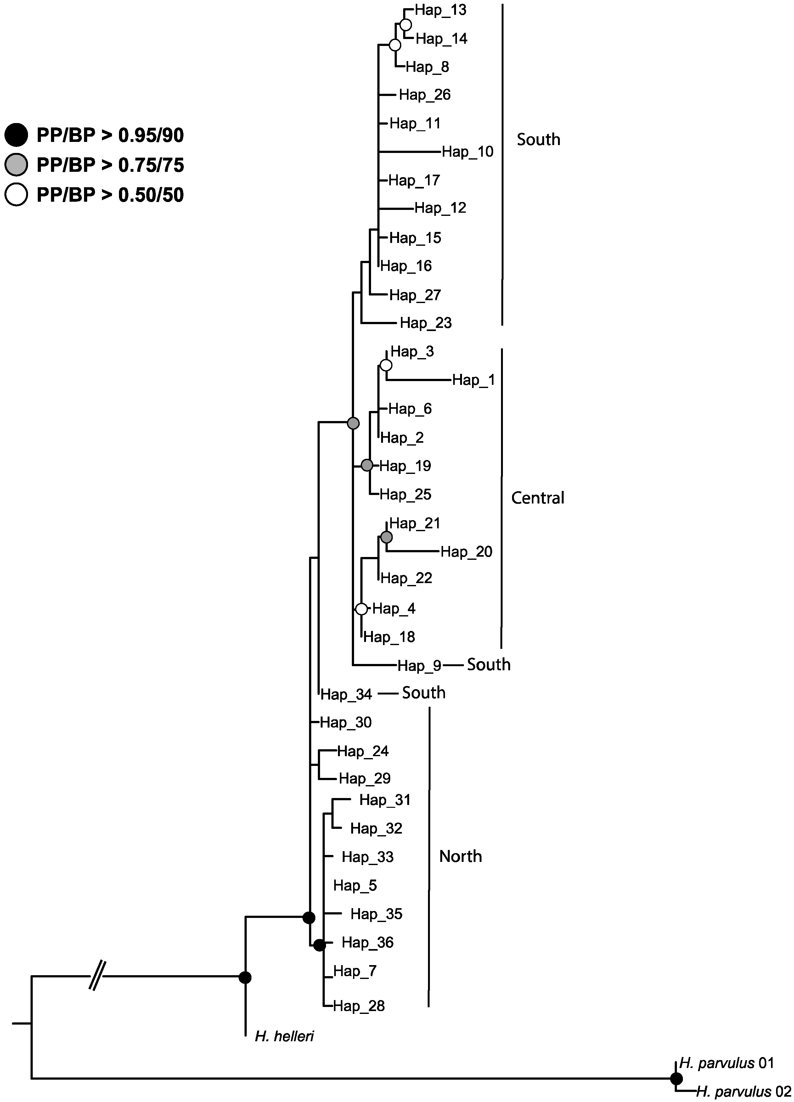
3.1. Strong but Unevenly Distributed Population Structure Across the Range for Hydnorobius hydnorae

Analyzing a 460 base-pair fragment of Cyt-B in 64 H. hydnorae weevil specimens, 36 mitochondrial DNA (mDNA) haplotypes were detected forming a single network with three main groups following a latitudinal pattern: The ‘southern group’ (SG), ‘central group’ (CG) and ‘northern group’ (NG; Figure 2B). The SG is composed of 14 haplotypes distributed exclusively south of 33° S. Within SG, one of the most frequent and widespread haplotypes (H16) appears in an internal position at the core of a star-like network topology. Haplotype 11 is connected by one step to the central haplotype H16 and is shared by two sampling sites. Haplotype 9 is shared by two localities too, but it is connected by many steps to the central haplotype, H16. The rest of the haplotypes of the SG are exclusive to single localities (i.e., H12, H13, H26, H27). The CG consists of nine haplotypes distributed in the central-west area in the septentrional Monte. Each locality presented exclusive haplotypes; even the most frequent haplotype H4 is found in a single locality near to the northwest Monte boundary limit. All of the haplotypes of NG are present in the Chaco province (23–32° S). The most frequent NG haplotype, H5, is present in three southern localities of Chaco, appears at an internal position and forms the core of another star-like network topology. Haplotypes located at the center of star-like structures and with a wide geographic distribution are considered ancestral and good indicators of potential ancestral areas [23]. Haplotypes 31 and 32 are exclusively found in the north of the distribution.
The SAMOVA structure analysis showed an optimal partition of genetic diversity of K = 3 (FCT = 0.45, p < 0.0001), revealing three genetic groups mostly in concordance with the haplotype network (Figure 2A,B). The exception is the position of H25, a unique haplotype from Chancaní (CCH) that is grouped with other ‘northern group’ haplotypes in the SAMOVA analysis; however, it appears to be only a few mutational steps away from ‘central group’ haplotypes in the network.
Results for all AMOVA combinations of analyses are presented in Table 2. The significantly high variation found among localities (ΦST = 0.5345) without hierarchical levels assigned can be interpreted as a signal of population structure. This means that populations are highly differentiated and with infrequent migration (average migration rate, Nm = 0.109). More specifically, the structure appears as significant between the regional groupings as determined by SAMOVA, either considering or not considering the localities as units. It is not unexpected that when analyzing the groupings as large populations, a significant amount of variation is found between the groups (ΦST = 0.4709), however, a substantial amount of variation (52.91%) is also found within each of these groups of localities. The analysis among the locality groupings maintaining the locality delimitations indicates that a significant 44.8% of variation (ΦCT = 0.4488) is found among area groupings. The rest of the variation is divided between an average 15.32% among localities within each area, and 39.8% within populations. In summary, AMOVA results suggest that this weevil species presents population structure, which contains a geographic signal and is most likely represented by the phylogenetic relationships of the haplotypes.
The pairwise FST values among localities detailed in Table 3 and Figure 3, as well as the pairwise FST values among the three areas without the locality distinctions, illustrate the patterns of structure at smaller scales and reveal that the degree of isolation and structuring between localities is not homogeneous across the range. Pairwise FST values between the three areas each as a single unit are all significant, however the Northern area is the most distinct, with higher differentiation with the Central and Southern areas (FST N-C 0.5493; FST N-S 0.4999), while the haplotypes in Southern and Central areas are not as differentiated (FST S-C 0.3023). Values of pairwise FST between localities in different areas (inter-area values in Figure 3) are all larger than those among localities within any of the three areas, and a high proportion of them are significant (61.40%). In addition to being the most distinct, the Northern locality area displays the wider range of pairwise FST values between localities, including some of the larger pairwise differentiation indexes, and the largest proportion of within-area significant values (30%). The Central locality area displays lower differentiation values, with only 10% of them being significant. Finally, the Southern locality area appears the most homogeneous, with low and not significant pairwise FST values.
Results of the pairwise calculations of the number of migrants that localities exchange (Nm, Supplementary Table S1) are the inverse of those found for the pairwise FST values and support the same pattern of isolation between areas, with the Northern area more distinct and less homogeneous than the others. Similarly, even though the Nm values are highly variable among all localities, inter-area values are much lower than within-area values supporting less connectivity and therefore genetic structure among the three areas. Some pairwise Nm values (inf) may indicate that those locality pairs are behaving as a single population.
Phylogenetic relationships among haplotypes inferred by ML and BI are shown in Figure 4. Both reconstructions retrieved all H. hydnorae haplotypes nested in a strongly supported clade (BP = 89, PP = 0.99) and are congruent with the topology resulting from the haplotype network, and largely in agreement with SAMOVA groupings (Figure 2A,B). These analyses provide high support for a split between most of the haplotypes of the NG (except for H24, H25, H29 and H30). The rest of haplotypes appeared in a clade with moderate support that corresponds with the groupings for CG and SG.

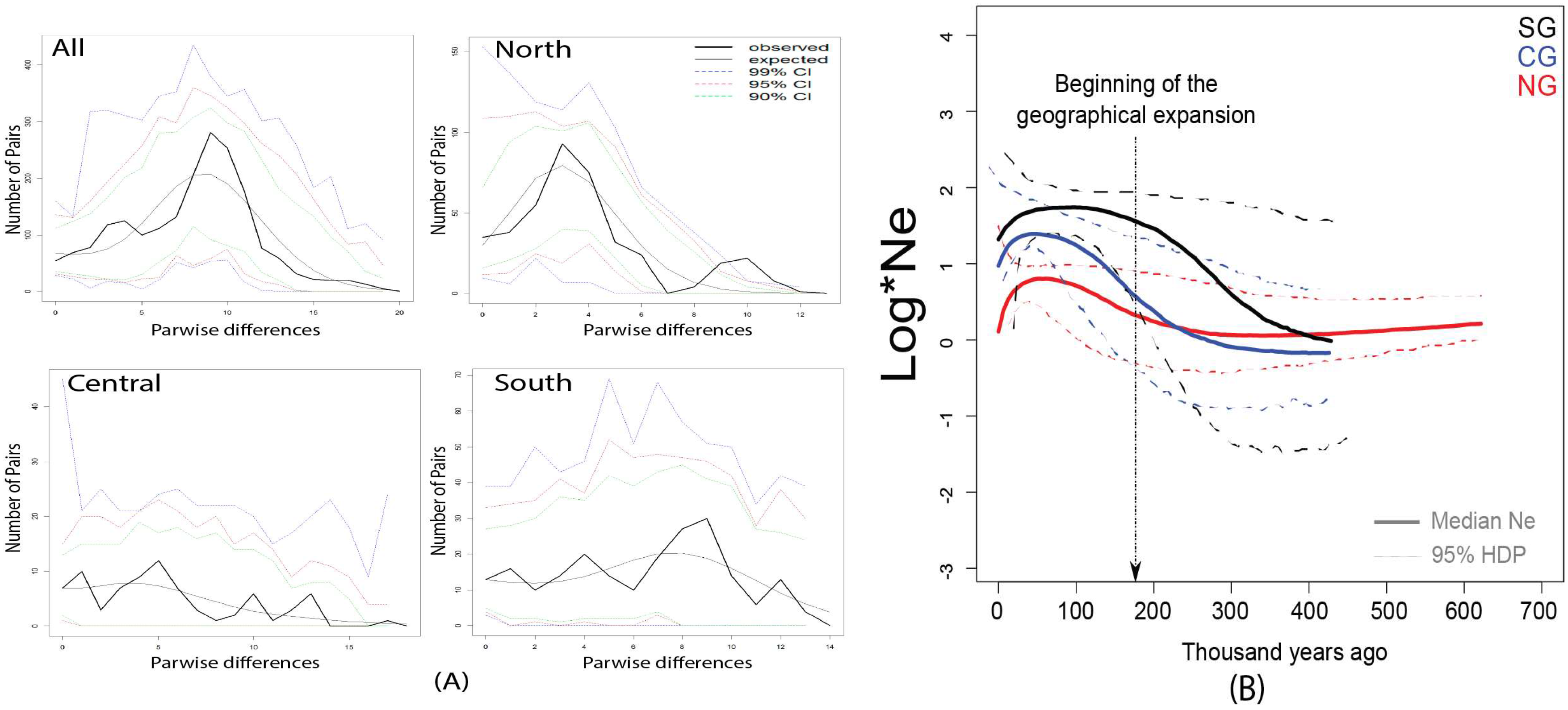
3.2. Weak Signals of Population Expansion for the Hydnorobius Hydnorae Population as a Whole

Considering all localities as a single population, the haplotype diversity (h) was 0.5714 and the nucleotide diversity (π) was 0.0185. This pattern of substantial haplotype diversity with moderate nucleotide diversity could be a signature of population growth from a smaller ancestral population size. The suggestion might be that since the origin of H. hydnorae, enough time has elapsed to produce some haplotype variation via mutation (h) but not enough for the accumulation of large differences in sequence (π). Table 4 shows the haplotype and nucleotide diversity for each locality. All localities present high values of haplotype diversity and low values of nucleotide diversity.
Results of Tajima’s D and Fu’s F tests are shown in Table 4. For the entire sample, both Tajima’s and Fu’s neutrality tests were negative, with only the FS index being significant (DS = −1.5263, p = 0.111; FS = −16.064, p < 0.05). Some of the individual localities presented negative values for these statistics, but none of them were significant. Given that many of the individual locality sample sizes are small, estimates of population size changes will be more accurately derived, in this case, from the analysis of locality groupings. Analyses of localities grouped according to the three SAMOVA groupings also produce negative neutrality indexes, with only one significant Fs value for SG.
The mismatch distribution analysis performed for the locality groupings presents clear evidence of stable demographic history (Figure 5A) with multimodal mismatch patterns and non-significant raggedness values (NG: r = 0.087, p = 0.35; CG: r = 0.091, p = 0.59; SG: r = 0.009, p = 0.91). However, the mismatch distribution analysis for the entire sample of this weevil species does not immediately suggest a stable demographic history, since it showed a tendency to a unimodal distribution (Figure 5A). Even though the raggedness value was low and non-significant (r = 0.0063; p = 0.87), the shape of the distribution could suggest that, as a whole, populations of this weevil species are not in demographic stability, probably reflecting some demographic expansion, as also suggested by the results of Fu’s F tests for the whole group.
For the three genetic groups detected (NG, CG, SG), the BSPs suggest an initial period of stability between 600 and 200 kya, followed by weak growth in population size since ~200 kya until ~30 kya where a decrease in the effective size is detected (Figure 5B). This pattern is common for the three groups but more pronounced in SG and CG.

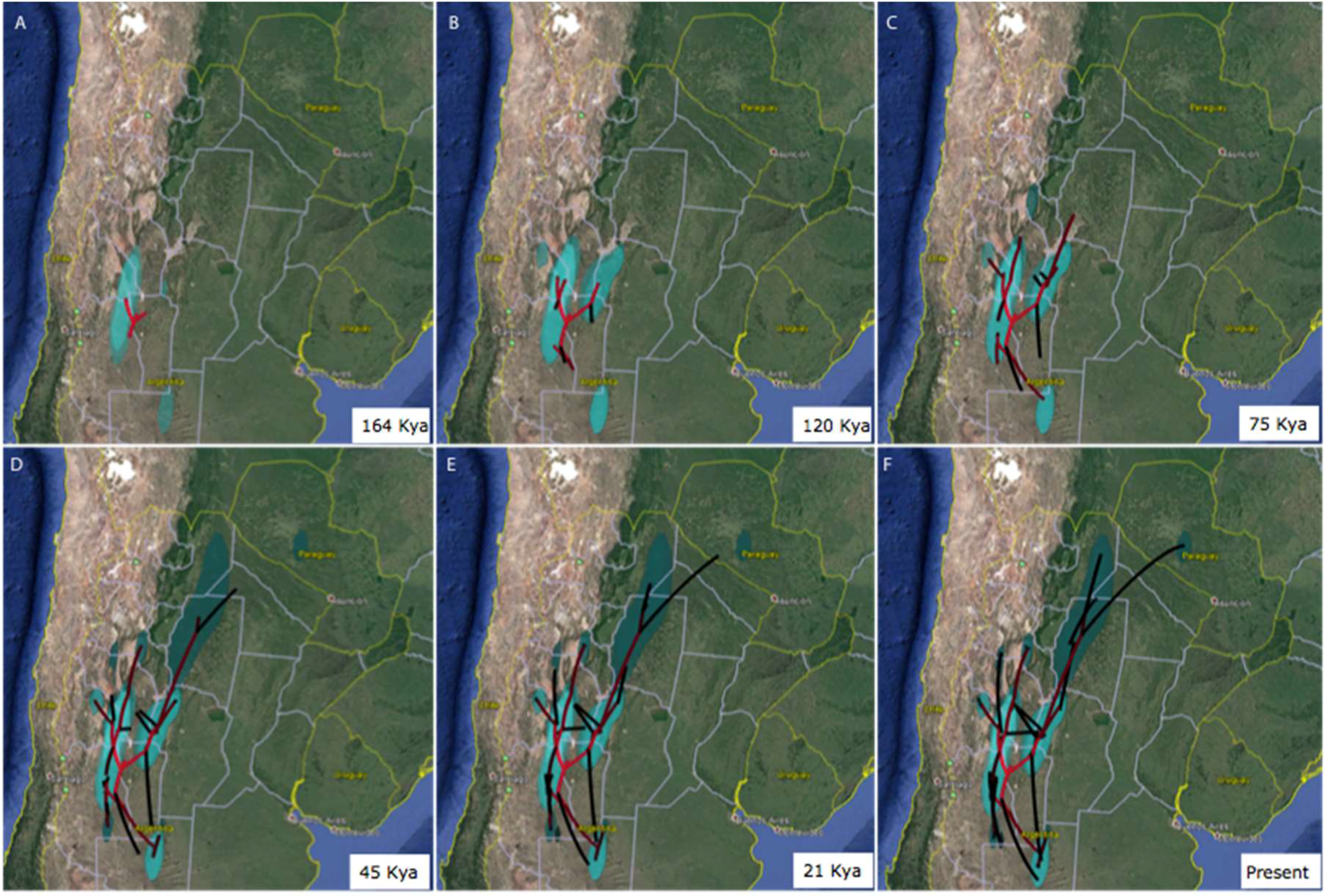
3.3. Area of Origin and North-South Axis of Spatio-Temporal Diffusion for H. hydnorae

The spatial diffusion rate for the Cyt-B matrix for H. hydnorae was estimated as 2175 km/My (95% HPD = 1040 km/My, 3301 km/My). The RRW diffusion model inferred a first step of the expansion consisting of two simultaneous colonization paths towards the North and South from the area of origin in northwestern San Luis Province (32°44′ S 66°55′ W) beginning at around 206–143 kya (Figure 6A). The Northern colonization route split into two independent areas: towards the West reaching the Northern Monte, and towards the East reaching the southern edge of the Chaco biogeographic province. The Southern colonization route established the ancestors in the austral part of Northern Monte (Figure 6B).
After this initial expansion around 128–79 kya, the Northern groups expanded into multiple areas and at a faster rate than those from the South; this is especially true for those from the Northeast (Figure 6C).
Around 79 kya, the ancient Northern group would have covered most of Western Chaco and the Northern Monte regions, while the Southern group would have reached the southern end of the current distribution of H. hydnorae (Figure 6D). Since 63 kya to the present, the colonizations were directed to the Northwest of Argentina and from the center of the Argentinian Chaco to the center of Paraguay. During this last period there are no expansions towards the South, but instead re-colonizations of the austral areas of Northern Monte from the areas near the center of dispersion of the species (Figure 6E,F).

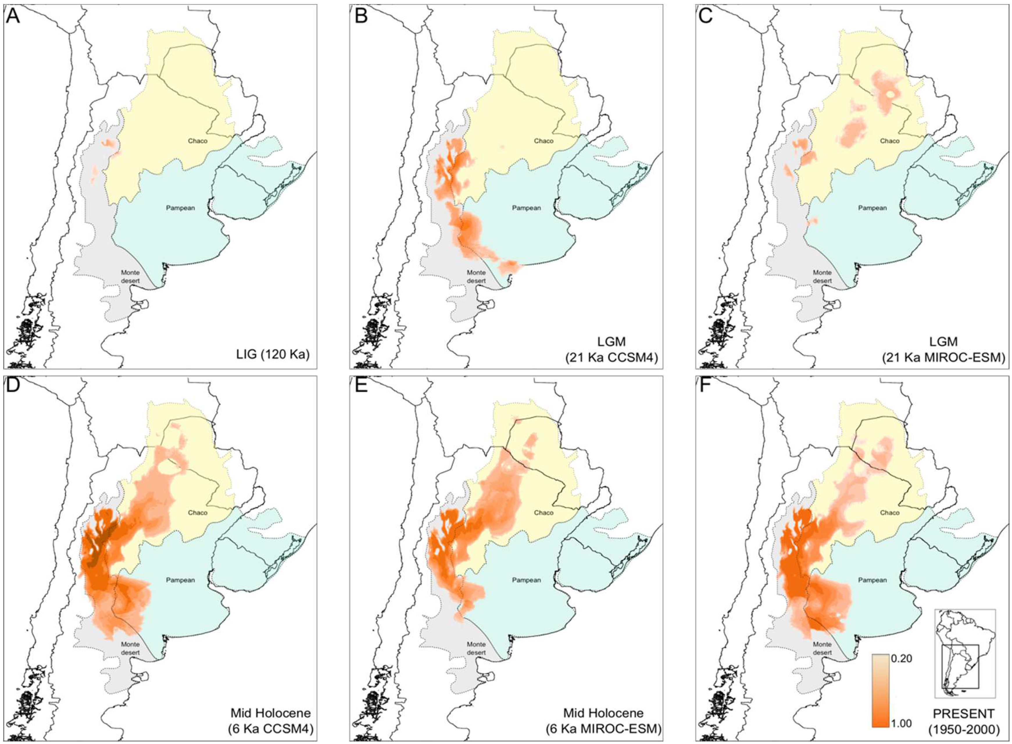
3.4. North-South Range Expansion in Prosopanche Americana, the Host of Hydnorobius hydnorae during 120 Kya

The average AUC obtained for the current climatic model (1959–2000) for P. americana was 0.9192 (± 0.031), indicating an optimal performance of the MaxEnt algorithm. The paleodistribution obtained for P. americana at 120 Kya during the LIG suggests a very restricted distribution in the Northern Monte (Figure 7A). Predictions at the LGM, under the CCSM4 simulation, suggest a southeastern range expansion in the southern portion of Northern Monte and west of Pampean biogeographic province with high-suitability values, while the MIROC-ESM climatic model suggests a northeastern range expansion in a fragmented scenario in the Chaco biogeographic province (Figure 7B,C). During the Mid-Holocene, both models suggest continuous expansions to the Northeast and Southeast (Figure 7D,E) approaching the current distribution of P. americana (Figure 7F). The PDM to current climatic conditions occupies a larger high-favorability area than at the LGM but smaller than in Mid-Holocene, suggesting range fragmentation mainly in the northern portion of the distribution in the Chaco region (Figure 7F).

4. Discussion

4.1. Genetic Structure and Geographic Expansions without Major Demographic Change Across the Range of Hydnorobius hydnorae

The weevil H. hydnorae is a univoltine beetle specifically associated to its host plant P. americana, [11,64] which in turn is parasite on the roots of Prosopis spp. (“Algarrobo” trees, Fabaceae) in arid and semiarid regions of the Monte, Chaco and Pampean biogeographic provinces. Although weevils of this species can fly, they do not present high vagility. Likewise, the dispersal capacity of P. americana may also be rather low, by means of endozoochory, carried by nocturnal mammals that eat the fruits [17]. Emergence of adults of H. hydnorae starting a new generation coincides with the emergence of new plants. The weevil’s low vagility and restrained biological habits may provide an explanation for the high degree of genetic structuring found across the range of H. hydnorae. Interestingly, the Northern haplogroup is the most structured and most distinct from the Central and Southern haplogroups, while it is also the one showing some early signals of rather weak population growth. However, most of the geographic expansion occurred after the growth pulses (220 kya), when there was effectively no growth occurring or even in the face of size reductions (30 kya). We find it intriguing that geographic expansion from ancestral areas to the edges of the distributions (see below) is uncoupled in time from any substantial demographic expansion. Studies on other species in the Monte desert describe the opposite pattern: demographic expansions occurring after sustained periods of range expansion [53].
The vicariant event described by Flores and Roig-Juñent [18] proposes a split of the Northern Monte from the remaining Southern areas, isolating Patagonia from Northern areas in Argentina. They attribute this event to marine transgressions that occurred 9.55 to 9.11 Mya, which are suggested by several sources of evidence [65]. Molecular phylogenetics for the Belidae estimated the age of origin of this weevil at about ~10 Mya [66,67]; thus, marine transgressions that occurred at ~9 Mya could have affected the distribution of H. hydnorae, generating a northern and southern pattern of distribution. This pattern of distribution could have also been later affected by volcanic and glacial periods, as has been proposed for other animals [68].
The sampled range of H. hydnorae spans the defined districts of Northern Monte, Western or Dry Chaco and Espinal of the Monte, Chaco and Pampean biogeographical provinces. Further subdivisions of the Monte area have been proposed based on vegetation [19] and in concordance with entomological evidence [18]. The phylogenetic relationships between H. hydnorae haplotypes, as well as the current structuring of the variation of H. hydnorae haplotypes into the three locality groups of NG, CG and SG, are quite concordant with current biogeographic regionalization. The Northern haplogroup occurs exclusively in the Chaco province, namely in the Dry Chaco, while the Central haplogroup resides mostly in the Northern Monte [19] and the Southern haplogroup occurs southward and eastward in Northern Monte and Espinal of the Pampean biogeographic province. These areas show a climatic transition from subtropical to temperate [69]. Separations such as the one we observe for H. hydnorae between the Central and Southern locality groups within the Monte region, north and south of 35° S, are common to a varied array of Monte inhabitants such as lizards, parrots and plants [26,70,71]. This is, to our knowledge, the first such example from an insect. The co-occurrence of such a genetic break in a disparate set of taxa has prompted suggestions of a shared regional history underlying these microevolutionary patterns, as well as those at a macroevolutionary level [26,72]. The Quarternary climatic history of the region includes severe glaciation patterns and shifts in the boundaries of ecotones [73]. On the other hand, the separation between the Northern and Central locality groups, each housed in the Dry Chaco and Northern Monte, respectively, could be mediated, in part, by the presence of the Famatina–Sañogasta Mountains, as observed for other Monte dwellers [68,74] and therefore be more independent of climatic patterns. However, a study on turtles that also finds the Northern Monte/Dry Chaco split has linked the separation to a vicariant event rooted in Plio-Pleistoce climatic changes [75].
Alternatively, the Northern area could have acted as a northern refuge from glacial periods (Pleistocene: 1.81–0.01 Mya) or Miocene periods of volcanic activity [76,77,78]. The idea of the Northern localities acting as refugia may be supported by the location of the ancestral haplotypes in the area, as well as by the location of the ancestral area selected by the Bayesian diffusion analysis.

4.2. Ancestral Weevil Haplotypes and Ancestral Areas for Hydnorobius hydnorae and Its Host Plant

In populations that present scarce or limited gene flow, the oldest and ancestral haplotypes are expected to be those with the most widespread geographic range [23]. Conversely, the haplotypes restricted to a single area are considered to have a recent origin [79]. Haplotype networks for H. hydnorae indicate that the most probable ancestral haplotypes are either H16 or H5, given that they are widespread across multiple localities and at the center of star-like topologies in the haplotype network in the SG and NG respectively. H16 is the most widespread SG southern haplotype distributed from the localities of El Durazno and La Maruja in La Pampa to Paso del Loro at the southern tip of Mendoza province (Figure 2A). H5 also is at the center of a star like structure (six other haplotypes derive from it) and is the most widely distributed NG haplotype present in Quines in San Luis, Chancaní in Córdoba and San Ramón in La Rioja, all localities within the Chaco Biogeographic province.
Bayesian diffusion analysis provides additional clues regarding the area of first expansion of H. hydnorae. The RRW model suggests that diffusion started at around 206–143 kya from northwestern San Luis province located within the Northern area, in agreement with the location of the more Northern putative ancestral haplotypes (H5). Despite the potential ancestral condition of H16, the RRW analyses that explicitly integrate geographic locations and coalescent history of haplotypes indicate that the ancestral area is further north with a higher posterior probability, compared to that of the area of prevalence of H16.
The predicted past distribution of the host plant P. americana during the LIG 130 kya shows that the most probable area of occurrence for this species in the north of the biogeographic region of Monte desert and close to the western edge of the Chaco region. The past distribution of P. americana and the ancestral range of H. hydnorae show a high degree of overlap suggesting an ancient association within concordant ancient ranges, as was expected under a coevolutionary or co-dispersal scenario between the weevil and its host plant.
In addition, information from paleoclimatic conditions and the fossil record indicates that plants of genus Prosopis (Fabaceae), the host of P. americana, were abundant during the Miocene (5–23 Mya) and Lower Pliocene (1–5 Mya) [80,81] in Northern Argentina. In essence, evidence suggests that the evolution and diversification of Prosopis took place jointly with the expansion of arid areas in the American continent, after the Andean uplift in the late Miocene [82]. This is because the uplift of the Andes caused the blocking of the more humid winds [83,84] and the expansion of xeric habitats. This provides evidence for the long-term persistence of a “three-way” interspecies interaction (Prosopis-Prosopanche-Hydnorobius) in the Monte desert. Some other enduring two-way associations between insects and South American plants have been reported for weevils and beetles feeding on relictual ancient conifers [85,86,87,88,89], and for two oil-collecting bee species and the perennial endemic herbs they pollinate [6]. More generally, an old history of specialized insect-plant interactions has been suggested as a main contributing factor to current biodiversity in the Patagonian region [90].

4.3. Concordant Weevil and Host Plant Diffusion-Expansion Patterns

Despite the caveats of the particular models used to generate either dispersal patterns or niche projections [91], we see the dispersal of weevil and host plant across space and time as interestingly synchronized. Both members of the interaction have concomitantly broadened their range from a common ancestral area following a Northern and a Southern track. If we were to think of Prosopanche flowers as Hydnorobius weevils’ habitat, then a specialist species adapted to this moving habitat must track its habitat spatially if it is to persist [92]. Nevertheless, tracking the host plant in its dispersal does not preclude the original locations from continuing being occupied, so in essence what we are detecting are not range shifts but matching ranges, not an unusual result in specialist interactions [93].
However, long-term co-dispersal seems to be less common. Passive co-dispersal of mutualists has been observed in other insect-plant interactions, such as ants and mealybugs [94]. There seems to be no evidence that Hydnorobius adults or larvae are passively dispersed with Prosopanche. Given the weevil life cycle, so tightly linked to the host-plant as an obligate relationship at least for the weevil (which is entirely dependent on the Prosopanche for feeding, mating and larval development), we are inclined to suggest that active host tracking by Hydnorobius adults has led to the observed matching ranges. Similar generation times and modest dispersal capacity for both interacting species can further contribute to concordant dispersal patterns through space and time [95].
Even though episodes of environmental change have been suggested to create opportunities for host-switching during geographical expansion in host-parasite systems [96], it appears that host switching during the recorded history of geographic expansion and environmental changes in Hydnorobius did not occur, or occurred just to an extremely similar and phylogenetically close species such as P. bonacinai [11]. Rather, what we observe is a long trajectory of host-tracking through space and time, where the weevil has expanded its geographic range following its host plant, but without significant demographic growth. Other monophagous insects show local population size closely following the cover of its food plant, so that host plant density could be a reliable prognosticator of the population size of the specialist insect [97,98]. Additionally, insect expansion rates have been suggested to be likely to increase with habitat availability [99]. One potential explanation for geographic dispersal without any substantial population growth in Hydnorobius could be that the scarcity of the host plant itself allows for maintenance of slow expansion rates and stable populations, with no need for significant demographic growth pulses to support geographic range expansion.

5. Conclusions

Genetic structuring of H. hydnorae populations across Northern Argentina appears to have arisen through a combination of the weevil’s low vagility and specialist larval feeding habits, with cycles of historical climatic changes. Such an obligate association has persisted across glacial cycles, generating a close match in the dispersal histories of H. hydnorae and its host plant P. americana in space and time, illustrating a long standing dependent association. Similarly, aspects of the population biology, ecology and life history of the host plant itself appear to influence the historical demography of the weevil allowing for range expansion without any substantial population growth.

Supplementary Materials

The following are available online at https://www.mdpi.com/1424-2818/10/2/33/s1, Table S1: Pairwise Nm estimates among 18 localities of H. hydnorae. Inter-area contrasts are not shaded while those within areas are shaded by locality area as defined through SAMOVA analysis (North: light gray; Central: dark gray; South: medium gray).

Author Contributions

A.S.S., A.E.M. and M.S.F. conceived and designed the experiments; M.S.F. and N.R. performed the experiments; A.S.S., M.S.F., N.R. and M.C.B. analyzed the data; A.E.M. and A.S.S. contributed reagents and materials; A.S.S., N.R., A.E.M., M.C.B. and M.S.F. wrote the paper.

Acknowledgments

We gratefully acknowledge the laboratory assistance of M. Sijapati, M. Maraorgarti, P. Mandal (Wellesley College) and L. Caeiro (Laboratorio de Biología Molecular, Universidad Nacional de Córdoba). This work was supported with Brachman Hoffman funds through Wellesley College (M.S.F. and A.S.S.) and through a travel award to M.S.F. from the Society of Systematic Biologists. This research received continued support from the National Scientific and Technical Research Council (CONICET, Argentina) through doctoral (to N.R. and M.S.F.) and postdoctoral (M.C.B.) fellowships, and research grants (PIPs 6766 and 00162 to A.E.M. and PIP 00765 to A. Cocucci) and by the National Agency of Promotion of Science (ANPCyT, Argentina) through grant PICTs 2011-2573 and 2016-2798 (to A.E.M.) and PICT-2015-3325 (to A. Cocucci). Additional aid to field and lab work of N.R. and M.C.B. was received from ANPCyT grant PICT 2015-3089 (to A. Sércic). We are very thankful to A. Cocucci for providing Figure 1C and assisting with questions regarding flower morphology and pollination. Our gratitude also goes to many people who assisted in field trips and/or provided specimens for molecular work, especially M. F. Fernández-Campón, D. R. Maddison, M. B. Maldonado, F. C. Ocampo, S. A. Roig-Juñent, G. Salazar. All authors acknowledge research facilities and support from their respective institutions.

Conflicts of Interest

The authors declare no conflict of interest. The founding sponsors had no role in the design of the study; in the collection, analyses, or interpretation of data; in the writing of the manuscript, and in the decision to publish the results.

References

  1. Futuyma, D.J.; Agrawal, A.A. Macroevolution and the biological diversity of plants and herbivores. Proc. Natl. Acad. Sci. USA 2009, 106, 18054–18061. [Google Scholar] [CrossRef] [PubMed]
  2. Toju, H.; Sota, T. Phylogeography and the geographic cline in the armament of a seed-predatory weevil: Effects of historical events vs. natural selection from the host plant. Mol. Ecol. 2006, 15, 4161–4173. [Google Scholar] [CrossRef] [PubMed]
  3. De-la-Mora, M.; Piñero, D.; Oyama, K.; Farrell, B.; Magallón, S.; Núñez-Farfán, J. Evolution of Trichobaris (Curculionidae) in relation to host plants: Geometric morphometrics, phylogeny and phylogeography. Mol. Phylogenet. Evol. 2018, 124, 37–49. [Google Scholar] [CrossRef] [PubMed]
  4. Alvarez, N.; Kjellberg, F.; Mckey, D.; Hossaert-McKey, M. Phylogeography and historical biogeography of obligate specific mutualisms. In The Biogeography of Host-Parasite Interactions; Oxford University Press: Oxford, UK, 2010; pp. 31–39. ISBN 978-0-19-956134-6. [Google Scholar]
  5. Gavin, D.G.; Fitzpatrick, M.C.; Gugger, P.F.; Heath, K.D.; Rodríguez-Sánchez, F.; Dobrowski, S.Z.; Hampe, A.; Hu, F.S.; Ashcroft, M.B.; Bartlein, P.J. Climate refugia: Joint inference from fossil records, species distribution models and phylogeography. New Phytol. 2014, 204, 37–54. [Google Scholar] [CrossRef] [PubMed]
  6. Sosa-Pivatto, M.; Cosacov, A.; Baranzelli, M.C.; Iglesias, M.R.; Espíndola, A.; Sérsic, A.N. Do 120,000 years of plant–pollinator interactions predict floral phenotype divergence in Calceolaria polyrhiza? A reconstruction using species distribution models. Arthropod-Plant Interact. 2017, 11, 351–361. [Google Scholar] [CrossRef]
  7. Thompson, A.R.; Thacker, C.E.; Shaw, E.Y. Phylogeography of marine mutualists: Parallel patterns of genetic structure between obligate goby and shrimp partners. Mol. Ecol. 2005, 14, 3557–3572. [Google Scholar] [CrossRef] [PubMed]
  8. Valiente-Banuet, A.; Rumebe, A.V.; Verdú, M.; Callaway, R.M. Modern Quaternary plant lineages promote diversity through facilitation of ancient Tertiary lineages. Proc. Natl. Acad. Sci. USA 2006, 103, 16812–16817. [Google Scholar] [CrossRef] [PubMed]
  9. Kuschel, G. Oxycorynus missionis spec. nov. from NE Argentina, with key to the South American species of Oxycoryninae (Coleoptera: Belidae). Acta Zool. Lilloana 1995, 43, 45–48. [Google Scholar]
  10. Kuschel, G. Nemonychidae, Belidae y Oxycorynidae de la fauna chilena, con algunas consideraciones biogeográficas. Investig. Zool. Chile 1959, 5, 229–271. [Google Scholar]
  11. Ferrer, M.S.; Marvaldi, A.E. New host plant and distribution records for weevils of the genus Hydnorobius (Coleoptera: Belidae). Rev. Soc. Entomol. Argent. 2010, 69, 271–274. [Google Scholar]
  12. Nickrent, D.L.; Blarer, A.; Qiu, Y.-L.; Soltis, D.E.; Soltis, P.S.; Zanis, M. Molecular data place Hydnoraceae with Aristolochiaceae. Am. J. Bot. 2002, 89, 1809–1817. [Google Scholar] [CrossRef] [PubMed]
  13. Naumann, J.; Salomo, K.; Der, J.P.; Wafula, E.K.; Bolin, J.F.; Maass, E.; Frenzke, L.; Samain, M.-S.; Neinhuis, C.; Wanke, S. Single-copy nuclear genes place haustorial Hydnoraceae within Piperales and reveal a Cretaceous origin of multiple parasitic angiosperm lineages. PLoS ONE 2013, 8, e79204. [Google Scholar] [CrossRef] [PubMed]
  14. Massoni, J.; Forest, F.; Sauquet, H. Increased sampling of both genes and taxa improves resolution of phylogenetic relationships within Magnoliidae, a large and early-diverging clade of angiosperms. Mol. Phylogenet. Evol. 2014, 70, 84–93. [Google Scholar] [CrossRef] [PubMed]
  15. Byng, J.W.; Chase, M.W.; Christenhusz, M.J.; Fay, M.F.; Judd, W.S.; Mabberley, D.J.; Sennikov, A.N.; Soltis, D.E.; Soltis, P.S.; Stevens, P.F. An update of the Angiosperm Phylogeny Group classification for the orders and families of flowering plants: APG IV. Bot. J. Linn. Soc. 2016, 181, 1–20. [Google Scholar]
  16. Cocucci, A.E. Estudios en el género Prosopanche (Hydnoraceae). I. Revisión taxonómica. Kurtziana 1965, 2, 53–74. [Google Scholar]
  17. Cocucci, A.E.; Cocucci, A.A. Prosopanche (Hydnoraceae): Somatic and reproductive structures, biology, systematics, phylogeny and potentialities as a parasitic weed. In Congresos y Jornadas-Junta de Andalucía (España); JA, DGIA: New York, NY, USA, 1996. [Google Scholar]
  18. Roig-Juñent, S.; Flores, G.; Claver, S.; Debandi, G.; Marvaldi, A. Monte Desert (Argentina): Insect biodiversity and natural areas. J. Arid Environ. 2001, 47, 77–94. [Google Scholar] [CrossRef]
  19. Roig, F.A.; Roig-Juñent, S.; Corbalán, V. Biogeography of the Monte desert. J. Arid Environ. 2009, 73, 164–172. [Google Scholar] [CrossRef]
  20. Vogt, C. Composición de la flora vascular del Chaco Boreal, Paraguay III. Dicotyledoneae: Gesneriaceae–Zygophyllaceae. Steviana 2013, 5, 5–40. [Google Scholar]
  21. Bruch, C. Coleópteros fertilizadores de “Prosopanche Burmeisteri” De Bary. Physis 1923, 7, 82–88. [Google Scholar]
  22. Marvaldi, A.E. Larval morphology and biology of oxycorynine weevils and the higher phylogeny of Belidae (Coleoptera, Curculionoidea). Zool. Scr. 2005, 34, 37–48. [Google Scholar] [CrossRef]
  23. Avise, J.C. Phylogeography: The History and Formation of Species; Harvard University Press: Cambridge, MA, USA, 2000; ISBN 0-674-66638-0. [Google Scholar]
  24. Sérsic, A.N.; Cosacov, A.; Cocucci, A.A.; Johnson, L.A.; Pozner, R.; Avila, L.J.; Sites, J.W.; Morando, M. Emerging phylogeographical patterns of plants and terrestrial vertebrates from Patagonia. Biol. J. Linn. Soc. 2011, 103, 475–494. [Google Scholar] [CrossRef]
  25. Turchetto-Zolet, A.C.; Pinheiro, F.; Salgueiro, F.; Palma-Silva, C. Phylogeographical patterns shed light on evolutionary process in South America. Mol. Ecol. 2013, 22, 1193–1213. [Google Scholar] [CrossRef] [PubMed]
  26. Baranzelli, M.C.; Cosacov, A.; Ferreiro, G.; Johnson, L.A.; Sérsic, A.N. Travelling to the south: Phylogeographic spatial diffusion model in Monttea aphylla (Plantaginaceae), an endemic plant of the Monte Desert. PLoS ONE 2017, 12, e0178827. [Google Scholar] [CrossRef] [PubMed]
  27. Morrone, J.J. Biogeographical regionalisation of the Neotropical region. Zootaxa 2014, 3782, 1–110. [Google Scholar] [CrossRef] [PubMed]
  28. Rokas, A.; Ladoukakis, E.; Zouros, E. Animal mitochondrial DNA recombination revisited. Trends Ecol. Evol. 2003, 18, 411–417. [Google Scholar] [CrossRef]
  29. Kraytsberg, Y.; Schwartz, M.; Brown, T.A.; Ebralidse, K.; Kunz, W.S.; Clayton, D.A.; Vissing, J.; Khrapko, K. Recombination of human mitochondrial DNA. Science 2004, 304, 981. [Google Scholar] [CrossRef] [PubMed]
  30. Avise, J.C.; Arnold, J.; Ball, R.M.; Bermingham, E.; Lamb, T.; Neigel, J.E.; Reeb, C.A.; Saunders, N.C. Intraspecific phylogeography: The mitochondrial DNA bridge between population genetics and systematics. Annu. Rev. Ecol. Syst. 1987, 18, 489–522. [Google Scholar] [CrossRef]
  31. Crozier, R.H.; Crozier, Y.C. The cytochrome b and ATPase genes of honeybee mitochondrial DNA. Mol. Biol. Evol. 1992, 9, 474–482. [Google Scholar] [PubMed]
  32. Simon, C.; Frati, F.; Beckenbach, A.; Crespi, B.; Liu, H.; Flook, P. Evolution, weighting, and phylogenetic utility of mitochondrial gene sequences and a compilation of conserved polymerase chain reaction primers. Ann. Entomol. Soc. Am. 1994, 87, 651–701. [Google Scholar] [CrossRef]
  33. Hall, T.A. BioEdit: A user-friendly biological sequence alignment editor and analysis program for Windows 95/98/NT. In Nucleic Acids Symposium Series; Information Retrieval Ltd.: London, UK, 1999; Volume 41, pp. 95–98. [Google Scholar]
  34. Rozas, J.; Sánchez-DelBarrio, J.C.; Messeguer, X.; Rozas, R. DnaSP, DNA polymorphism analyses by the coalescent and other methods. Bioinformatics 2003, 19, 2496–2497. [Google Scholar] [CrossRef] [PubMed]
  35. Bandelt, H.-J.; Forster, P.; Röhl, A. Median-joining networks for inferring intraspecific phylogenies. Mol. Biol. Evol. 1999, 16, 37–48. [Google Scholar] [CrossRef] [PubMed]
  36. Leigh, J.W.; Bryant, D. Popart: Full-feature software for haplotype network construction. Methods Ecol. Evol. 2015, 6, 1110–1116. [Google Scholar] [CrossRef]
  37. Dupanloup, I.; Schneider, S.; Excoffier, L. A simulated annealing approach to define the genetic structure of populations. Mol. Ecol. 2002, 11, 2571–2581. [Google Scholar] [CrossRef] [PubMed]
  38. Excoffier, L.; Lischer, H.E.L. Arlequin suite ver 3.5: A new series of programs to perform population genetics analyses under Linux and Windows. Mol. Ecol. Resour. 2010, 10, 564–567. [Google Scholar] [CrossRef] [PubMed]
  39. Flores, G.E.; Roig-Juñent, S. Cladistic and biogeographic analyses of the Neotropical genus Epipedonota Solier (Coleoptera: Tenebrionidae), with conservation considerations. J. N. Y. Entomol. Soc. 2001, 109, 309–336. [Google Scholar] [CrossRef]
  40. Drummond, A.J.; Rambaut, A. BEAST: Bayesian evolutionary analysis by sampling trees. BMC Evol. Biol. 2007, 7, 214. [Google Scholar] [CrossRef] [PubMed] [Green Version]
  41. Darriba, D.; Taboada, G.L.; Doallo, R.; Posada, D. jModelTest 2: More models, new heuristics and parallel computing. Nat. Methods 2012, 9, 772. [Google Scholar] [CrossRef] [PubMed]
  42. Tracer. Available online: http://tree.bio.ed.ac.uk/software/tracer/ (accessed on 23 March 2018).
  43. FigTree. Available online: http://tree.bio.ed.ac.uk/software/figtree/ (accessed on 23 March 2018).
  44. Guindon, S.; Dufayard, J.-F.; Lefort, V.; Anisimova, M.; Hordijk, W.; Gascuel, O. New Algorithms and Methods to Estimate Maximum-Likelihood Phylogenies: Assessing the Performance of PhyML 3.0. Syst. Biol. 2010, 59, 307–321. [Google Scholar] [CrossRef] [PubMed]
  45. Nei, M.; Kumar, S. Molecular Evolution and Phylogenetics; Oxford University Press: Oxford, UK, 2000; ISBN 0-19-535051-0. [Google Scholar]
  46. Tajima, F. Statistical method for testing the neutral mutation hypothesis by DNA polymorphism. Genetics 1989, 123, 585–595. [Google Scholar] [PubMed]
  47. Harpending, H.C. Signature of ancient population growth in a low-resolution mitochondrial DNA mismatch distribution. Hum. Biol. 1994, 66, 591–600. [Google Scholar] [PubMed]
  48. Mckenna, D.D.; Wild, A.L.; Kanda, K.; Bellamy, C.L.; Beutel, R.G.; Caterino, M.S.; Farnum, C.W.; Hawks, D.C.; Ivie, M.A.; Jameson, M.L.; et al. The beetle tree of life reveals that Coleoptera survived end-Permian mass extinction to diversify during the Cretaceous terrestrial revolution. Syst. Entomol. 2015, 40, 835–880. [Google Scholar] [CrossRef]
  49. Zhang, S.-Q.; Che, L.-H.; Li, Y.; Pang, H.; Ślipiński, A.; Zhang, P. Evolutionary history of Coleoptera revealed by extensive sampling of genes and species. Nat. Commun. 2018, 9, 205. [Google Scholar] [CrossRef] [PubMed]
  50. Lemey, P.; Rambaut, A.; Welch, J.J.; Suchard, M.A. Phylogeography Takes a Relaxed Random Walk in Continuous Space and Time. Mol. Biol. Evol. 2010, 27, 1877–1885. [Google Scholar] [CrossRef] [PubMed]
  51. Pybus, O.G.; Tatem, A.J.; Lemey, P. Virus evolution and transmission in an ever more connected world. Proc. R. Soc. B 2015, 282, 20142878. [Google Scholar] [CrossRef] [PubMed]
  52. Drummond, A.J.; Ho, S.Y.W.; Phillips, M.J.; Rambaut, A. Relaxed Phylogenetics and Dating with Confidence. PLoS Biol. 2006, 4, e88. [Google Scholar] [CrossRef] [PubMed] [Green Version]
  53. Camargo, A.; Werneck, F.P.; Morando, M.; Sites, J.W.; Avila, L.J. Quaternary range and demographic expansion of Liolaemus darwinii (Squamata: Liolaemidae) in the Monte Desert of Central Argentina using Bayesian phylogeography and ecological niche modelling. Mol. Ecol. 2013, 22, 4038–4054. [Google Scholar] [CrossRef] [PubMed]
  54. Bielejec, F.; Rambaut, A.; Suchard, M.A.; Lemey, P. SPREAD: Spatial phylogenetic reconstruction of evolutionary dynamics. Bioinformatics 2011, 27, 2910–2912. [Google Scholar] [CrossRef] [PubMed]
  55. Guisan, A.; Thuiller, W. Predicting species distribution: Offering more than simple habitat models. Ecol. Lett. 2005, 8, 993–1009. [Google Scholar] [CrossRef]
  56. Graham, C.H.; Ron, S.R.; Santos, J.C.; Schneider, C.J.; Moritz, C. Integrating phylogenetics and environmental niche models to explore speciation mechanisms in dendrobatid frogs. Evolution 2004, 58, 1781–1793. [Google Scholar] [CrossRef] [PubMed]
  57. Naumann, J.; Der, J.P.; Wafula, E.K.; Jones, S.S.; Wagner, S.T.; Honaas, L.A.; Ralph, P.E.; Bolin, J.F.; Maass, E.; Neinhuis, C. Detecting and characterizing the highly divergent plastid genome of the nonphotosynthetic parasitic plant Hydnora visseri (Hydnoraceae). Genome Biol. Evol. 2016, 8, 345–363. [Google Scholar] [CrossRef] [PubMed]
  58. WorldClim—Global Climate Data|Free climate data for ecological modeling and GIS. Available online: http://www.worldclim.org/ (accessed on 22 March 2018).
  59. Hijmans, R.J.; Cameron, S.E.; Parra, J.L.; Jones, P.G.; Jarvis, A. Very high resolution interpolated climate surfaces for global land areas. Int. J. Climatol. 2005, 25, 1965–1978. [Google Scholar] [CrossRef]
  60. Phillips, S.J.; Anderson, R.P.; Schapire, R.E. Maximum entropy modeling of species geographic distributions. Ecol. Model. 2006, 190, 231–259. [Google Scholar] [CrossRef]
  61. Anderson, R.P.; Gonzalez, I., Jr. Species-specific tuning increases robustness to sampling bias in models of species distributions: An implementation with Maxent. Ecol. Model. 2011, 222, 2796–2811. [Google Scholar] [CrossRef]
  62. Otto-Bliesner, B.L.; Marshall, S.J.; Overpeck, J.T.; Miller, G.H.; Hu, A. Simulating Arctic climate warmth and Icefield retreat in the last interglaciation. Science 2006, 311, 1751–1753. [Google Scholar] [CrossRef] [PubMed]
  63. Schneider, S.; Excoffier, L. Estimation of past demographic parameters from the distribution of pairwise differences when the mutation rates vary among sites: Application to human mitochondrial DNA. Genetics 1999, 152, 1079–1089. [Google Scholar] [PubMed]
  64. Marvaldi, A.E.; Oberprieler, R.G.; Lyal, C.H.C.; Bradbury, T.; Anderson, R.S. Phylogeny of the Oxycoryninae sensu lato (Coleoptera: Belidae) and evolution of host-plant associations. Invertebr. Syst. 2006, 20, 447–476. [Google Scholar] [CrossRef]
  65. Werneck, F.P. The diversification of eastern South American open vegetation biomes: Historical biogeography and perspectives. Quat. Sci. Rev. 2011, 30, 1630–1648. [Google Scholar] [CrossRef]
  66. Ferrer, M.S. Molecular Systematics and Evolution of Belidae, with Special Reference to Oxycoryninae (Coleoptera: Curculionoidea). Ph.D. Thesis, Universidad Nacional de Cuyo, Mendoza, Argentina, 2011. [Google Scholar]
  67. Ferrer, M.S.; Sequeira, A.S.; Marvaldi, A.E. Host associations in ancient weevils: A phylogenetic perspective on Belidae and Nemonychidae. Diversity, Under preparation.
  68. Yoke, M.M.; Morando, M.; Avila, L.J.; Sites, J.W., Jr. Phylogeography and genetic structure in the Cnemidophorus longicauda complex (Squamata, Teiidae). Herpetologica 2006, 62, 420–434. [Google Scholar] [CrossRef]
  69. Morrone, J.J. Biogeographic Areas and Transition Zones of Latin America and the Caribbean Islands Based on Panbiogeographic and Cladistic Analyses of the Entomofauna. Annu. Rev. Entomol. 2006, 51, 467–494. [Google Scholar] [CrossRef] [PubMed]
  70. Morando, M.; Avila, L.J.; Baker, J.; Sites, J.W., Jr. Phylogeny and phylogeography of the Liolaemus darwinii complex (Squamata: Liolaemidae): Evidence for introgression and incomplete lineage sorting. Evolution 2004, 58, 842–861. [Google Scholar] [CrossRef] [PubMed]
  71. Masello, J.F.; Quillfeldt, P.; Munimanda, G.K.; Klauke, N.; Segelbacher, G.; Schaefer, H.M.; Failla, M.; Cortés, M.; Moodley, Y. The high Andes, gene flow and a stable hybrid zone shape the genetic structure of a wide-ranging South American parrot. Front. Zool. 2011, 8, 16. [Google Scholar] [CrossRef] [PubMed]
  72. Vuilleumier, B.S. Pleistocene changes in the fauna and flora of South America. Science 1971, 173, 771–780. [Google Scholar] [CrossRef] [PubMed]
  73. Markgraf, V. Late and postglacial vegetational and paleoclimatic changes in subantarctic, temperate, and arid environments in Argentina. Palynology 1983, 7, 43–70. [Google Scholar] [CrossRef]
  74. Rivera, P.C.; González-Ittig, R.E.; Robainas Barcia, A.; Trimarchi, L.I.; Levis, S.; Calderón, G.E.; Gardenal, C.N. Molecular phylogenetics and environmental niche modeling reveal a cryptic species in the Oligoryzomys flavescens complex (Rodentia, Cricetidae). J. Mammal. 2018, 99, 363–376. [Google Scholar] [CrossRef]
  75. Sánchez, J. Variabilidad Genética, Distribución y Estado de Conservación de Las Poblaciones de Tortugas Terrestres Chelonoidis chilensis (Testudines: Testudinidae) Que Habitan en la República Argentina. Ph.D. Thesis, Universidad Nacional de La Plata, Buenos Aires, Argentina, 2013. [Google Scholar]
  76. Nullo, F.E.; Stephens, G.C.; Otamendi, J.; Baldauf, P.E. El volcanismo del Terciario superior del sur de Mendoza. Rev. Asoc. Geol. Argent. 2002, 57, 119–132. [Google Scholar]
  77. Sruoga, P.; Guerstein, P.; Bermudez, A. Riesgo volcánico. In XII Congreso Geológico Argentino; Ramos, V., Ed.; Asociación Geológica Argentina: Mendoza, Argentina, 1993; pp. 659–667. [Google Scholar]
  78. Ortiz-Jaureguizar, E.; Cladera, G.A. Paleoenvironmental evolution of southern South America during the Cenozoic. J. Arid Environ. 2006, 66, 498–532. [Google Scholar] [CrossRef]
  79. Neigel, J.E.; Ball, R.M.; Avise, J.C. Estimation of single generation migration distances from geographic variation in animal mitochondrial DNA. Evolution 1991, 45, 423–432. [Google Scholar] [CrossRef] [PubMed]
  80. Anzótegui, L.M.; Garralla, S.S.; Herbst, R. Fabaceae de la Formación El Morterito (Mioceno superior) del valle del Cajón, provincia de Catamarca, Argentina. Ameghiniana 2007, 44, 183–196. [Google Scholar]
  81. Anzótegui, L.M.; Horn, Y.; Herbst, R. Paleoflora (Fabaceae y Anacardiaceae) de la Formación Andalhuala (Plioceno Inferior), provincia de Catamarca, Argentina. Ameghiniana 2007, 44, 525–535. [Google Scholar]
  82. Catalano, S.A.; Vilardi, J.C.; Tosto, D.; Saidman, B.O. Molecular phylogeny and diversification history of Prosopis (Fabaceae: Mimosoideae). Biol. J. Linn. Soc. 2008, 93, 621–640. [Google Scholar] [CrossRef]
  83. Pascual, R.; Ortiz Jaureguizar, E.; Prado, J.L. Land mammals: Paradigm for Cenozoic South American geobiotic evolution. Münch. Geowiss. Abh. 1996, 30, 265–319. [Google Scholar]
  84. Alberdi, M.T.; Bonnadona, F.P.; Ortiz Jaureguizar, E. Chronological correlation, paleoecology, and paleobiogeography of the late Cenozoic South American Rionegran land-mammal fauna: A review. Rev. Esp. Palent. 1997, 12, 249–255. [Google Scholar]
  85. Kuschel, G.; Poinar, G.O. Libanorhinus succinus gen. & sp. n. (Coleoptera: Nemonychidae) from Lebanese amber. Insect Syst. Evol. 1993, 24, 143–146. [Google Scholar]
  86. Kuschel, G.; May, B.M. Discovery of Palophaginae (Coleoptera: Megalopodidae) on Araucaria araucana in Chile and Argentina. N. Z. Entomol. 1996, 19, 1–13. [Google Scholar] [CrossRef]
  87. Farrell, B.D. “Inordinate fondness” explained: Why are there so many beetles? Science 1998, 281, 555–559. [Google Scholar] [CrossRef] [PubMed]
  88. Sequeira, A.S.; Normark, B.B.; Farrell, B.D. Evolutionary assembly of the conifer fauna: Distinguishing ancient from recent associations in bark beetles. Proc. R. Soc. Lond. B Biol. Sci. 2000, 267, 2359–2366. [Google Scholar] [CrossRef] [PubMed]
  89. Sequeira, A.S.; Farrell, B.D. Evolutionary origins of Gondwanan interactions: How old are Araucaria beetle herbivores? Biol. J. Linn. Soc. 2001, 74, 459–474. [Google Scholar] [CrossRef]
  90. Wilf, P.; Labandeira, C.C.; Johnson, K.R.; Cúneo, N.R. Richness of plant–insect associations in Eocene Patagonia: A legacy for South American biodiversity. Proc. Natl. Acad. Sci. USA 2005, 102, 8944–8948. [Google Scholar] [CrossRef] [PubMed]
  91. Peterson, A.T.; Soberón, J.; Pearson, R.G.; Anderson, R.P.; Martínez-Meyer, E.; Nakamura, M.; Araújo, M.B. Ecological Niches and Geographic Distributions (MPB-49); Princeton University Press: Princeton, NJ, USA, 2011; ISBN 1-4008-4067-8. [Google Scholar]
  92. Pease, C.M.; Lande, R.; Bull, J.J. A model of population growth, dispersal and evolution in a changing environment. Ecology 1989, 70, 1657–1664. [Google Scholar] [CrossRef]
  93. Keane, R.M.; Crawley, M.J. Exotic plant invasions and the enemy release hypothesis. Trends Ecol. Evol. 2002, 17, 164–170. [Google Scholar] [CrossRef]
  94. Gaume, L.; Matile-Ferrero, D.; Mckey, D. Colony foundation and acquisition of coccoid trophobionts by Aphomomyrmex afer (Formicinae): Co-dispersal of queens and phoretic mealybugs in an ant-plant-homopteran mutualism? Insectes Soc. 2000, 47, 84–91. [Google Scholar] [CrossRef]
  95. Waltari, E.; Perkins, S.L. In the hosts footsteps? Ecological niche modeling and its utility in predicting parasite distributions. In The Biolgeography of Host-Parasite Interactions; Oxford University Press: Oxford, UK, 2010; pp. 145–155. ISBN 978-0-19-956134-6. [Google Scholar]
  96. Hoberg, E.P.; Brooks, D.R. A macroevolutionary mosaic: Episodic host-switching, geographical colonization and diversification in complex host–parasite systems. J. Biogeogr. 2008, 35, 1533–1550. [Google Scholar] [CrossRef]
  97. Krauss, J.; Steffan-Dewenter, I.; Tscharntke, T. Landscape occupancy and local population size depends on host plant distribution in the butterfly Cupido minimus. Biol. Conserv. 2004, 120, 355–361. [Google Scholar] [CrossRef]
  98. León-Cortés Jorge, L.; Lennon Jack, J.; Thomas Chris, D. Ecological dynamics of extinct species in empty habitat networks. 2. The role of host plant dynamics. Oikos 2003, 102, 465–477. [Google Scholar] [CrossRef]
  99. Thomas, C.D.; Bodsworth, E.J.; Wilson, R.J.; Simmons, A.D.; Davies, Z.G.; Musche, M.; Conradt, L. Ecological and evolutionary processes at expanding range margins. Nature 2001, 411, 577–581. [Google Scholar] [CrossRef] [PubMed]
Figure 1. The plant Prosopanche americana (AC) and its associated weevil Hydnorobius hydnorae (DE). (A) Flower showing the open perianth and perigonial tube on top of the inferior ovary attached to a rhizome bearing haustorial roots; (B) Open flower showing the dome-like androecium releasing pollen and bearing a pair of mating H. hydnorae; (C) Development of the Prosopanche flower from bud (left) to open flower in stigmatic (middle) and staminal (right) phases (a, anther body; f, fenestrae connecting a and c; c, stigmatic chamber; s, receptive stigma; p, pollen); (D) H. hydnorae full-grown larva in decaying plant tissue; (E) H. hydnorae pupa in pupal cell and (F) Dorsal view of adult H. hydnorae.
Diversity 10 00033 g001
Figure 2. (A) Northwestern region of Argentina with all Hydnorobius hydnorae collecting localities. Details associated with locality codes can be found in Table 1. The larger shaded areas correspond to biogeographic provinces as in Morrone [27]. Pie charts indicate proportional presence of distinct Cytochrome B (Cyt-B) haplotypes in each locality. (B) Minimum spanning network showing all Cyt-B haplotypes for the 18 localities. Haplotype IDs are indicated by the circles and the size of the circles is proportional to the frequency of each haplotype. Dashes on the haplotype connections indicate the number of mutational steps between them. Sections of the network are colored according to the locality groups suggested by the SAMOVA analysis (K = 3). Those same colors are then depicted on the map grouping localities in three areas: North (red), Central (orange) and South (blue).
Diversity 10 00033 g002
Figure 3. Genetic differentiation between localities and locality areas. (A) Graphical depiction of pairwise Fst values between individual localities; (B) Box plots contrasting the distribution of pairwise Fst values between localities within each locality area, and those between areas (interarea), horizontal bars represent mean values for each group; (C) Graphical depiction of pairwise Fst values between locality areas.
Diversity 10 00033 g003
Figure 4. Bayesian inference (BI) and maximum likelihood (ML) topology illustrating relationships between individual haplotypes for H. hydnorae. Labeling of haplotypes by geographic group follows the regions depicted in Figure 2 and Table 1. Hydnorobius helleri and H. parvulus are used as outgroups. PP: posterior probabilities, PB: bootstrap resampling.
Diversity 10 00033 g004
Figure 5. Estimates of demographic expansion in Hydnorobius hydnorae. (A) Mismatch distributions for all samples as a single population (ALL) and for each locality group analyzed as a single unit (North, Central, South). To construct the curves of expected values, 10,000 datasets were simulated under a coalescent algorithm using estimated parameters based on a sudden demographic expansion [63]; (B) Bayesian skyline plots for all locality groups including confidence intervals. Arrow indicates the time estimate for geographic expansions derived from the Bayesian spatial diffusion analysis.
Diversity 10 00033 g005
Figure 6. Reconstructed spatio-temporal diffusion of H. hydnorae in South America, shown at six time slices: (A) 164 kya. (B) 120 kya. (C) 75 kya. (D) 45 kya. (E) 21 kya. (F) Present time. Lines represent branches of the maximum clade credibility tree (MCC), estimated with a Bayesian phylogeographic analysis in BEAST using a “Relaxed Random Walk” (RRW) model of continuous diffusion through time and space. Map data ©2018 Google Imagery ©2018 NASA, TerraMetrics.
Diversity 10 00033 g006
Figure 7. Spatial projections of Prosopanche americana climatic niche across several Quaternary climatic scenarios. (A) Last Interglacial maximum (LIG; 120 kya; CCMS); (B) Last Glacial Maximum (LGM; 21 kya; CCMS4); (C) Last Glacial Maximum (LGM; 21 kya; MIROC-ESM); (D) Mid-Holocene (6 kya, CCMS4); (E) Mid-Holocene (6 kya, MIROC-ESM); (F) Current conditions (average 1950–2000). Dotted lines indicate biogeographical regionalization and orange hues signals the climatic suitability for P. americana.
Diversity 10 00033 g007
Table 1. Locality information for all sampled specimens of Hydnorobius hydnorae organized by geographic area and by locality groupings from the SAMOVA K = 3 analysis. Population codes reflect province and locality name as in Figure 2. N indicates sample size per locality.
Province and Locality NamePopulation CodeCoordinatesN
NorthLa Rioja: San RamónLSRS 30° 22.002′; W 66° 52.002′4
San Luis: QuinesSLQUIS 32° 17.472′; W 65° 50.982′5
Córdoba: ChancaníCCHS 31° 22.584′; W 65° 28.812′4
Córdoba: Árbol blancoCABS 30° 9.06′; W 64° 4.404′5
Paraguay: HayesPHAYS 23° 4.818′; W 59° 13.272′3
Santiago del Estero: Aurora-HuayapampaSAUHUS 27° 25.416′; W 64° 16.686′5
Salta: La UniónSLUS 23° 45.918′; W 63° 4.914′1
Chaco: Taco PozoCHTPS 25° 40.74′; W 63° 7.8′2
CentralCatamarca: Pio BrizuelaCBRS 27° 49.878′; W 66° 12,16′3
Catamarca: TinogastaCTIS 28° 4.99′; W 67° 34.002′4
San Juan: BermejoSBES 31° 31.998′; W 67° 24′3
San Juan: HuacoSHUS 30° 9′; W 68° 34.998′3
SouthMendoza: DivisaderoMDIS 33° 11.4′; W 67° 51′5
Mendoza: Reserva de la Biósfera ÑacuñánMNAS 34° 3′; W 67° 57′4
Mendoza: Paso del LoroMPDS 35° 39.672′; W 67° 33,492′5
La Pampa: ChacharramendiLPCHAS 37° 24.372′; W 65° 18.39′ 1
La Pampa: El DuraznoLPDZOS 36° 40.448′; W 65° 17.346′ 3
La Pampa: La MarujaLPMARS 35° 37.62′; W 64° 50.418′3
Table 2. Hierarchical analysis of molecular variance (AMOVA) for H. hydnorae across 18 localities. Tests were performed for regional groups as determined by the SAMOVA analysis (northern; central and southern), and for all localities without hierarchical levels. Asterisks (*) denote significance level (p ≤ 0.05).
Source of Variation% of VariationFixation Indices (Φ-Statistics)
Among all localities without hierarchical levels53.45ΦST = 0.5345 *
Within Localities46.55
Among regional groups as single large populations47.09ΦST = 0.4709 *
Within regional groups52.91
Among SAMOVA proposed groupings44.88ΦCT = 0.4488 *
Among localities within groups15.32ΦSC = 0.2780 *
Within localities39.80ΦST = 0.6020 *
Table 3. Pairwise FST estimates among 18 Localities of H. hydnorae sampled. Inter-area contrasts are not shaded while those within areas are shaded by locality area as defined through SAMOVA analysis (Northern: light gray; Central: dark gray; Southern: medium gray). Asterisks (*) denote significance level values (p ≤ 0.05).
CAB0.398 *0
PHAY0.436 *0.793 *0
SAUHU−0.0130.553 *0.681 *0
SLU−0.2200.715100
CHTP0.1780.779 *10.28600
SLQUI0.060.5810.680.20.3350.5080
LSR−0.2390.330.353 *0−0.20.1520.060
CBR0.130.0330.0320.0450.0980.050.040.1520
CTI0.070.01300.02000.0180.0760.0470
SHU0.10.0310.0280.0430.090.0470.0390.1190.1450.0650
SBE0.20.0330.0230.0530.0660.0360.0440.2230.2120.1180.1940
MDI0.270.10.1290.1320.5110.1770.1050.3040.2230.1840.1990.5560
MPD0.170.060.0680.0780.150.0870.0650.1860.1440.1240.140.386−0.1540
MNA0.120.050.0550.0560.1130.0650.050.1460.1060.0560.1010.1320.1360.2150
LPDZO0.40.090.080.1150.3690.1140.0910.5330.1610.0910.1510.407−0.0510.0050.0650
LPMAR0.090.0280.0170.0340.0330.020.030.1210.080.0220.0720.1090.0360.0540.116−0.0590
LPCHA0.180.02200.034000.0310.2130.19700.1070.083−0.0140.30.4460.1410.686
Table 4. Genetic diversity and Neutrality tests (Tajima’s Ds and Fu’s Fs) per H. hydnorae locality and per SAMOVA defined locality group. (n: number of individuals per locality; h: haplotype diversity; π: nucleotide diversity; K: average number of pairwise differences).
Tajima’s DsFu’s Fs
Area/PopulationnhKπDsp ValueFsp Value
LSR40.83332.66670.0351−0.31450.5330.81140.568
SLQUI50.80002.00000.0048−1.12400.071−1.01160.114
CCH41.00005.1667 0.0123−0.52810.453−0.48050.205
CAB50.40001.60000.0038−1.09380.0802.20240.830
PHAY30.33330.00000.00000.00001N/AN/A
SAUHU50.40001.80000.00431.57270.9652.42850.859
SLU1N/AN/AN/AN/AN/AN/AN/A
CHTP20.50000001N/AN/A
North290.44823.82760.0091−1.00180.161−3.73140.086
CBR31.00004.00000.05260.00000.5512.30310.543
CTI40.50002.50000.0329−0.79680.1662.59800.859
SBE30.66670.66670.00880.000010.0000N. A.
SHU30.833312.08330.1590−1.41040.0783.06880.092
Central130.69235.43590.0129−0.84450.208−1.51520.201
MDI50.90003.20000.0421−0.81730.149−1.01240.106
MNA40.70001.40000.01840.00000.9481.06090.561
MPD50.80001.60000.02100.69900.7850.27640.523
LPCHA1N/AN/AN/AN/AN/AN/AN/A
LPDZO316.00000.01420.000010.58780.400
LPMAR30.66672.00000.00470.000011.60940.701
South 220.66676.29050.0149−0.96510.172−3.42860.007
ALL630.57147.82180.0185−1.52630.111−16.064<0.05

