Linking Diversity and Differentiation

Abstract

Generally speaking, the term differentiation refers to differences between collections for the distribution of specified traits of their members, while diversity deals with (effective) numbers of trait states (types). Counting numbers of types implies discrete traits such as alleles and genotypes in population genetics or species and taxa in ecology. Comparisons between the concepts of differentiation and diversity therefore primarily refer to discrete traits. Diversity is related to differentiation through the idea that the total diversity of a subdivided collection should be composed of the diversity within the subcollections and a complement called “diversity between subcollections”. The idea goes back to the perception that the mixing of differentiated collections increases diversity. Several existing concepts of “diversity between subcollections” are based on this idea. Among them, β-diversity and fixation (inadvertently called differentiation) are the most prominent in ecology and in population genetics, respectively. The pertaining measures are shown to quantify the effect of differentiation in terms of diversity components, though from a dual perspective: the classical perspective of differentiation between collections for their type compositions, and the reverse perspective of differentiation between types for their collection affiliations. A series of measures of diversity-oriented differentiation is presented that consider this dual perspective at two levels of diversity partitioning: the overall type or subcollection diversity and the joint type-subcollection diversity. It turns out that, in contrast with common notions, the measures of fixation (such as $F_{ST}$ or $G_{ST}$) refer to the perspective of type rather than subcollection differentiation. This unexpected observation strongly suggests that the popular interpretations of fixation measures must be reconsidered.

1. Introduction

Structural aspects of biological variation (genetic, phenotypic, species, taxa, etc.) are traditionally assessed by comparing three levels that result from division of collections of organisms into subcollections: variation in the total collection, variation within subcollections, and variation between subcollections. In population genetics, variation is measured in terms of genetic traits, and the collections of interest are populations or metapopulations with subpopulations as subcollections. At higher levels of organization, ecological research is typically concerned with species as the source of biological variation that may be characteristically distributed over the communities of a defined region. In this case communities form the subcollections of a collection that is determined by a region. Whenever any of the following considerations applies equally to population genetic, ecological or to even more encompassing fields of research, the terms trait, collection, and subcollection will be used without further specification. This is chiefly motivated by the fact that the terms “diversity” and “differentiation” have a conceptual basis of sufficient breadth to imply methods of measurement that apply to a large variety of problems (up to information theoretic concepts). Once recognized this may help in solving long-lasting debates and revealing so far overlooked principles shared by the disciplines.

Variation within and between subcollections are commonly considered as two components that complement each other with respect to the variation in the total collection. In the field of population genetics, this perception became manifest in Wright’s F-statistics (as summarized in his 1978 book [1], also see Weir [2]) and Nei’s analysis of gene diversity [3]. While F-statistics rest on the additive decomposition of the variance of allele frequencies into its within and between populations components, the analysis of gene diversity reproduces this additive decomposition on the basis of probabilities of gene identity. In ecology, both multiplicative and additive complementation is used (however see [4]), where the three levels or components are referred to as α- (within subcollections), β- (between subcollections) and γ-diversity (total collection, following Whittaker’s [5] lead; for a discussion of the relation between multiplicative and additive complementation see Ricotta [6]).

Conceptual criticism of the various measures of variation in use concentrates largely on the between-subcollections component of the total variation. This component is usually specified in relative terms. In population genetics it is mostly measured by the proportion of the total variation due to differences between populations (variation between subcollections divided by the total variation, as in Wright’s $F_{ST}$ or Nei’s $G_{ST}$). Other approaches quantify the amount of variation between subcollections directly through the genetic differences (distances) between populations [7]. In ecology, β-diversity is mostly specified as the diversity of the total collection (γ) divided by the diversity within collections (α). It therefore measures the multiplicity of the total variation in relation to the variation within subcollections (for a brief review of different measures and interpretations of β-diversity see e.g., [4] or [8].

In essence, the criticism centers around the observation that the established measures of variation between subcollections do not appropriately reflect the differentiation in type distribution between subcollections. For $F_{ST}$, its creator Wright himself emphasized that “The fixation index ($F_{ST}$) is thus not a measure of differentiation in the sense implied in the extreme case by absence of any common allele” ([1], p. 82). Indeed, $F_{ST}$ assumes its maximum value only if all populations (subcollections) are monomorphic (and thus “fixed” for a single allele) with the possibility that almost all populations share the same allele. The same applies to $G_{ST}$. Differentiation between populations may thus be low for large values of these measures. The wide spread ignorance of this fact gave rise to several publications pointing out further undesirable consequences of misusing $F_{ST}$ and its relatives for the measurement of differentiation ([7, 9, 10, 11, 12, 13, 14], just to mention a few in addition to Wright’s initial admonition).

According to [4], a basic criterion for β-diversity is its independence from α-diversity. This criterion is not sufficiently realized by many indices as was demonstrated by Jost [15]. In fact, Jost’s demonstrations show that for some of the most frequently used indices, high species diversity in a region may imply low β-diversity among the communities (or samples) of the region despite the fact that the species spectra are strongly differentiated between the communities. Most of these problems, however, vanish if explicit measures of diversity are used [15]. Explicit measures of diversity are required to reflect numbers of types (effective numbers, numbers equivalents) in that they are greater than or equal to one, are smaller than or equal to the number of types of objects present in a collection, and equal that number only if all types are equally frequent. The use of explicit measures of diversity also helps in drawing formal connections between the amount of differentiation between communities and their β-diversity as is implicit in the analysis of Jost ([12], where his ${\Delta }_{ST}$ can be addressed as a measure of β-diversity). It is interesting to note that, even though β diversity and $F_{ST}$-related measures both refer to variation between subcollections, usage of the former seems to be restricted to ecological problems while applications of the latter seem to be limited to population genetic problems.

In all of these considerations, analyses of diversity are focused on the distribution of types within and between subcollections, where numbers and sizes of subcollections seem to play no special role. Analyses are thus focused on the diversity of types without explicit reference to the number and thus to the diversity of subcollections. Yet, both kinds of diversity may depend on each other. This becomes obvious when recalling that complete differentiation in type distribution between subcollections cannot be realized if there are less types than subcollections and that likewise complete fixation (monomorphism) among subcollections cannot be realized if there are more types than subcollections. It is therefore not surprising that supposed measures of monomorphism like $F_{ST}$ and its relatives produce notoriously low values for highly variable genetic traits recorded in comparatively small numbers of populations. Similarly, for comparable numbers of populations, genetic traits of low overall variability produce small measures of differentiation (like the distance-oriented measure δ of [7]).

In other words, type diversity and subcollection diversity may put constraints on the distribution of variation. To take this into account, two kinds of diversity have to be considered in addition to type diversity: subcollection diversity and joint type and subcollection diversity. These kinds of diversity do not explicitly enter current methods of diversity analysis. It will be shown that inclusion of all three kinds of diversity (type, subcollection, joint) allows for the design of strictly diversity-oriented measures of differentiation (like the D of Jost [12]) and measures of monomorphism (like the $F_{ST}$ relatives). By doing so, the present paper will draw on results obtained from a recently proposed association-oriented approach to an analysis of distributional characteristics of total variation over subcollections [16]. It turned out in this analysis that differentiation for type distribution between subcollections and apportionment of type variation to subcollections are dual perspectives. Since the apportionment perspective is aimed at the degree to which the overall variation is divided among (sub-)collections with the extreme that all variation exists among collections (no “variation within”), it directly relates to measures of monomorphism. Therefore, the duality of differentiation and monomorphism will be further developed in the present paper with reference to the measurement of diversity. By this, relationships between existing concepts and measures will be revealed and new methods of measuring and interpreting diversity will be made available.

2. General Characteristics of Diversity Measures

Measures of diversity are distinguished from measures of spread or dispersion (such as the statistical variance or other average differences) in that the former basically refer to counting numbers of types which are specified by the states of discrete traits. This does not exclude the possibility that certain measures of spread can be interpreted as measures of diversity [17, 18]. To consider variable frequencies of types in this concept of diversity, any pertaining index is required to fulfill the evenness condition. The condition consists of two requirements:

(a)

diversity never decreases as the difference in frequency between two types decreases while the sum of their frequencies remains the same;

(b)

for given number of types, diversity attains its maximum only if all types are equally frequent.

In requirement (a), constancy of the sum of the two frequencies is crucial in that it characterizes the change in frequencies as a replacement process. Only in this sense it is meaningful to state that diversity increases as types become more even in representation. Jost [19] pointed out that the evenness condition is known in economics under the “principle of transfers”, and he listed it as one of the four central conditions to be realized by what he called “measures of compositional complexity” (realization of the other three conditions — see [19], p. 927 — is always tacitly assumed in the present paper). Note that requirement (a) implies requirement (b) if diversity increases strictly as the frequency difference decreases. This more restrictive assumption is not made, since it would rule out the number of types as one of the routinely applied measures of diversity.

To firmly establish the connection to numbers of types, an index of diversity is required to allow for a one-to-one transformation into what is frequently called an “effective number” or “numbers equivalent”. In fact, the existence of such a transformation is implicit in the evenness condition as follows from consistent application of the general concept of “effective number” (which will be returned to later in a separate section; also see [20]). The index constitutes a measure of explicit diversity in the above sense if by itself it represents a numbers equivalent and therefore equals the number of types in case these types are evenly distributed (which is implicit in condition 6 of [19]). By definition, indices of diversity are bounded from below and assume their minimum $v_{min}$, say, only for monomorphism. For explicit measures of diversity $v_{min}=1$. The decision to use non-explicitly specified measures of diversity without transformation into their explicit versions strongly depends on the interpretability of their values. The work of Jost cited in the present paper provides many examples in which the use of explicit measures is compelling.

3. Diversity in Subdivided Collections

Diversity-oriented measures of differentiation can in fact be designed such that they rely chiefly on fulfillment of the evenness condition and allow for what will be called a “reference diversity”. To achieve the latter objective, consider a collection of individuals that is divided into subcollections. In the field of population biology or population genetics, an assemblage of populations (like a metapopulation) may be considered as a collection, the subcollections of which are specified by the individual populations. Subcollections can as well be addressed as subpopulations of an encompassing population that in turn specifies the collection. In ecology, subcollections usually appear as samples of species taken from a specified region, the latter defining the overall collection. The samples may be determined by species communities.

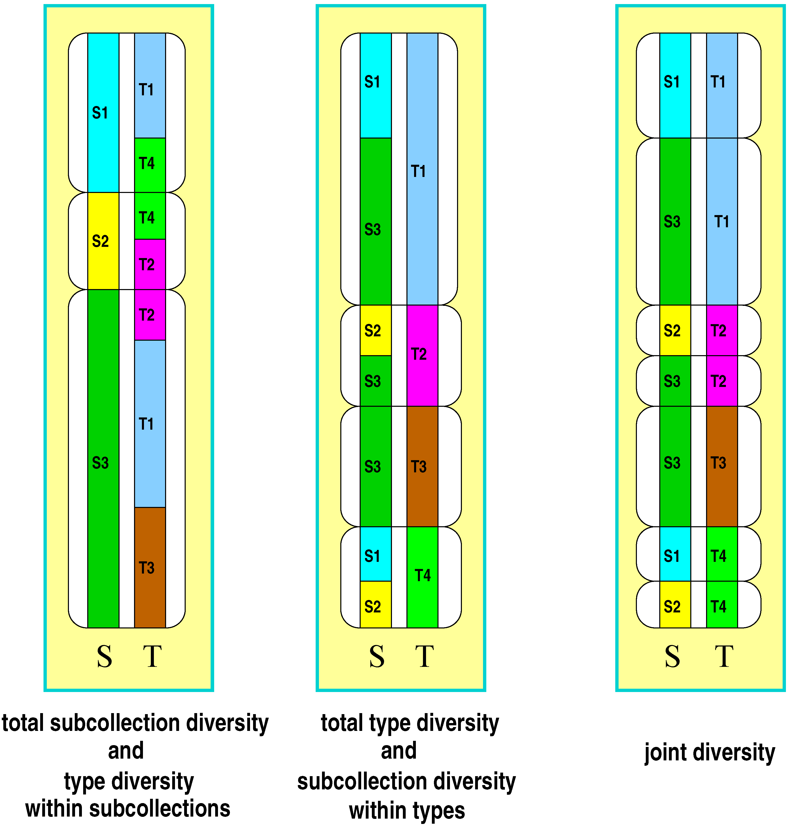
Following the approach of Gregorius [16], subdivision is taken into consideration in that each member of a collection is characterized by its affiliation to one of the subcollections (denoted by S) and by a trait, the states of which will be referred to as types (denoted by T). Individuals are therefore characterized by two attributes, type (T) and subcollection affiliation (S). According to these attributes a collection’s diversity can be organized into five basic components (for an illustration see Figure 1): (1) type diversity in the total collection, (2) type diversity within each subcollection, (3) diversity of subcollection affiliation in the total collection, (4) diversity of subcollection affiliation within each type, and (5) diversity of both attributes jointly. Measures of the components will be referred to as $v_T$, $v_T\left(j\right)$, $v_S$, $v_S\left(i\right)$ and $v_{TS}$ in the above order from (1) to (5), where j refers to the j-th subcollection $S_j$, and i refers to the i-th type $T_i$. $v_{TS}$ will be termed the joint diversity, in relation to which $v_T$ and $v_S$ appear as marginal diversities, and $v_T\left(j\right)$ and $v_S\left(i\right)$ appear as components of the respective marginal diversities. The evenness condition is required to hold for all of these components.

While type diversity within collections or subcollections is a familiar population genetic and ecological concept, diversity of subcollection affiliation of a type may sound strange at first sight. However, it also reflects common ecological ideas in various ways. One more prominent example is provided by the distinction between specialists and generalists, which essentially addresses situations where genotypes or species regularly occur either in only a narrow or in a wide spectrum of conditions. Identifying these conditions with habitats or subcollections, it becomes apparent that the continuum between specialists and generalists in fact addresses the number of habitats or subcollections in which types are found. Types may thus show various degrees of diversity with respect to their occurrence in habitats or subcollections. Joint diversities however seem to have played no role at all in ecological and population genetic research. Nevertheless they establish a basic link between the concepts of diversity and differentiation as will be demonstrated in the following.

Figure 1. Illustration of the five components of diversity in a subdivided collection (three subcollections $S1$ to $S3$, four types $T1$ to $T5$): subcollection diversity (left panel, left column), type diversity within subcollections (left panel, right column), type diversity within the total collection (middle panel, right column), subcollection diversity within types (middle panel, left column), joint type-subcollection diversity (right panel). The table provides the type, subcollection, and joint frequencies underlying the illustration.

Figure 1. Illustration of the five components of diversity in a subdivided collection (three subcollections $S1$ to $S3$, four types $T1$ to $T5$): subcollection diversity (left panel, left column), type diversity within subcollections (left panel, right column), type diversity within the total collection (middle panel, right column), subcollection diversity within types (middle panel, left column), joint type-subcollection diversity (right panel). The table provides the type, subcollection, and joint frequencies underlying the illustration.

	$S_1$	$S_2$	$S_3$	$\sum$
$T_1$	0.18	0.00	0.28	0.46
$T_2$	0.00	0.08	0.09	0.17
$T_3$	0.00	0.00	0.20	0.20
$T_4$	0.09	0.08	0.00	0.17
$\sum$	0.27	0.16	0.57	1.00

The evenness condition per se implies a number of generally desirable relationships between joint and marginal diversities. One of the direct consequences of the condition is that the introduction of a new type via partial replacement of an existing type increases (does not reduce) diversity. Subdivision of the states of a given trait into further states has the same effect. Hence, since subcollection affiliation can be considered as a subdivision of types, the joint diversity cannot be smaller than the type diversity, i.e., $v_{TS}\ge v_T$. For complete differentiation between subcollections, each type occurs in only one subcollection. Subcollection affiliation does therefore not subdivide types, so that in this case (and only in this case) $v_{TS}=v_T$. For reasons of symmetry in the attributes T and S, the same argument implies $v_{TS}\ge v_S$ with equality only if each subcollection consists of a single type (is fixed or monomorphic for a particular type). Thus, $v_{TS}\ge max\{v_T,v_S\}$. Recall that complete differentiation can be described by $v_S\left(i\right)=v_{min}$ for all types i while monomorphism of all subcollections is indicated by $v_T\left(j\right)=v_{min}$ for all subcollections j (with $v_{min}=1$ for explicit measures of diversity).

Because the two attributes can be looked at in a symmetrical way, the case of monomorphism (or fixation) can as well be conceived of as complete differentiation, provided types are distinguished for their subcollection affiliations (though this is an uncommon perspective). From this reverse perspective, types are completely differentiated for their subcollection affiliations if different types never occur in the same subcollection. This further emphasizes the duality of the differentiation perspective and the fixation (monomorphism) perspective [16].

Another simple consequence of complete differentiation between subcollections is $v_T\ge v_S$ with equality only if all subcollections are monomorphic. This follows from $v_{TS}\ge max\{v_T,v_S\}$ and from $v_{TS}=v_T$ by assumption. Under this premise, $v_T=v_S$ only if $v_{TS}=v_S$, which in turn implies complete differentiation between types for subcollection affiliations and thus monomorphism of all subcollections. The intuitively evident dual statement reads $v_S\ge v_T$ if and only if all subcollections are monomorphic. Note that these results are consequences solely of the evenness condition.

4. Reference Diversities: The Basis for Measuring the Effects of Differentiation

So far, diversity has been considered to measure variation within a given group of objects. Wordings like “diversity between groups” lack proper meaning in this context. The rational underlying this wording can probably be approached most consistently with reference to the general perception that any mixing of collections that are differentiated for their types must imply an increase in diversity as compared to the constituent collections. In particular, adding to a collection a more diverse one should result in a higher diversity in the mixture than in the less diverse collection. Obviously, this includes the possibility that the diversity of the mixture exceeds that of all of its constituent collections (as is obvious from the mixture of monomorphic collections). Yet, the diversity of a mixture may also be smaller than that of some of its components. In a mixture of three collections, the smallest consisting of two equally frequent types and the other two being both much larger and monomorphic for one of the two types, the smallest collection is clearly more diverse than the mixture of the three.

Hence, the perception that mixing of differentiated collections increases diversity basically depends on a special reference to be determined from among the diversities and sizes of the constituent collections. By definition, this reference diversity is not smaller than the smallest diversity in the collections, and it is not allowed to be affected by differences between the collections. Such differences should be detectable only from comparison of the diversity of the mixture with the reference diversity.

The latter distinguishes the diversity-oriented concept of differentiation fundamentally from the distance-oriented concept. In the distance-orientation, differences in frequency distribution of types between collections enter directly the measurement of differentiation. Multiple collections are considered through the distances between individual collections and the union of their respective remainders (see [7]). Distances are not measured between a mixture of collections and the frequency distribution of types in some reference collection. For two collections, in particular, their distance does not depend on their sizes. This is different in the diversity-orientation, where the diversity of the mixture of two collections strongly depends on the proportion by which the two collections are represented in the mixture (provided the collections are differentiated).

Strictly speaking, diversity-oriented measures of differentiation aim at assessing the gain in diversity due to mixing collections that differ in their frequency distributions of types. The magnitude of this gain is evaluated in relation to the diversities within the constituent collections. In contrast, distance-oriented measures serve the primary assessment of differentiation. They are largely independent of diversities but they affect the diversity of mixtures. Therefore, diversity-oriented measures of differentiation need not comply with the all of the conditions that are indispensable for distance-oriented measures. For example, partial replacement of extant types by new types necessarily increases diversity and can never lower distance-oriented differentiation. Yet, the effect on diversity-oriented measures of differentiation is not clear, since both the diversity of the mixture and the within collection diversities increase as a consequence of the replacement.

Usage of the term “differentiation” in connection with measures based on diversities may therefore be considered inappropriate. Because of common notions, however, the term will be retained together with the adjective “diversity-oriented”. Moreover, it is conceivable that special diversity indices meet several conditions that are considered desirable for distance-oriented measures of differentiation ([15], p. 2436, right column, provided arguments for why this may apply to Shannon-Wiener entropy or to other indices when equal weights are given to subcollections). It is essential to keep this in mind in all of the subsequent deliberations.

The reference diversity is usually conceived of as “diversity within subpopulations” (in population genetics) or referred to as “α-diversity” (in ecology). The gain in total diversity due to differentiation between subcollections is captured by the notion of β-diversity in ecology. As was conclusively argued by Jost [15], α and β components of diversity should be independent, and this is reflected by the above requirement on a suitable reference diversity. On the other hand, the reference must relate to the extremes of distributions of variation over subcollections, provided the extremes are reflected independently in the subcollections. One of these extremes is realized in the absence of differentiation, where all subcollections equal the total collection. The other extreme is reached if all subcollections are monomorphic.

By these explanations, a reference diversity that is suitable for an assessment of the effects of differentiation between the components of a subdivided collection should at a minimum fulfill the following requirements: (R1) it should never exceed the diversity of the total collection with equality only if all subcollections show identical type distributions, (R2) it should equal the minimum diversity $v_{min}$ only if all subcollections are monomorphic, and (R3) it should depend only on the diversities within the subcollections and on the relative subcollection sizes, it should equal the diversities within the subcollections if they are all equal, and it should not be smaller than the smallest diversity within the subcollections.

Reference diversities can be determined in a dual manner for both attributes, type and subcollection affiliation. In the following, reference diversities for types in subcollections will be denoted by $v_{T|S}$, and $v_{S|T}$ will stand for reference diversities of subcollection affiliation in types. The above requirements can then be stated as:

(R1)

$v_T\ge v_{T|S}$, $v_S\ge v_{S|T}$ with equality only in the absence of differentiation (stochastic independence of T and S),

(R2)

$v_{T|S}=v_{min}$ if and only if $v_T\left(j\right)=v_{min}$ for all j, and $v_{S|T}=v_{min}$ if and only if $v_S\left(i\right)=v_{min}$ for all i,

(R3)

$\left(i\right)$$v_{T|S}$ depends solely on the $v_T\left(j\right)$’s and the relative subcollection sizes, $v_{S|T}$ depends solely on the $v_S\left(i\right)$’s and the relative type frequencies, $\left(ii\right)$ $v_T\left(j\right)=c_T$ for all j implies $v_{T|S}=c_T$, and $v_S\left(i\right)=c_S$ for all i implies $v_{S|T}=c_S$, $\left(iii\right)$ $v_{T|S}\ge {min}_j{v}_T\left(j\right)$ and $v_{S|T}\ge {min}_i{v}_S\left(i\right)$.

A diversity measure (whether explicit or not) that is operational in analyses of differentiation should thus allow for reference diversities characterized by the requirements (R1) to (R3). Recall that $v_T$ and $v_{T|S}$ correspond to γ- and α-diversity in ecology. Accordingly, the quotient $v_T/v_{T|S}$ is commonly addressed as a measure of β-diversity (though this should be restricted to explicit measures of diversity, as argued by Jost [15]. Requirement (R3), in particular, allows for references that are designed as generalized means of the diversities within the subcollections. This reflects the requirement that references do not depend on the amount of differentiation between subcollections.

The requirements imply constraints that not all diversity measures may comply with. Thus, (R1) in combination with (R3)$\left(iii\right)$ implies that $v_T\ge {min}_j{v}_T\left(j\right)$ and $v_S\ge {min}_i{v}_S\left(i\right)$ (which is intuitively compelling). Moreover, if $v_T\left(j\right)=v_T$ for all j, then $v_{T|S}=v_T$ by (R3)$\left(ii\right)$, so that by (R1) the subcollections are not differentiated. Hence, the condition $v_T\left(j\right)=v_T$ for all j is equivalent to the absence of differentiation between subcollections (which in turn implies $v_S\left(i\right)=v_S$ for all i).

5. Diversity-oriented Measures of Differentiation

Relationships between differentiation and diversity that follow the perception that the mixing of collections should increase diversity can be looked at in different ways. One way focuses on the enumeration of types that specifically add to differences between subcollections. Ideally such types are “private” (or unique) to a single subcollection in the sense that they are absent in all other subcollections. This wording reflects one of the most common views of β-diversity. Since the underlying idea is to enumerate types, explicit measures of diversity are given preference. Hence, privateness of type i shows as $v_S\left(i\right)=1$, and it indicates that the i-th type occurs in exactly one subcollection (is absent in the remainder of the collection). Since $v_S\left(i\right)$ increases with the number of subcollections in which the i-th type is present, this diversity component can as well be considered as being inversely related to the degree of “privateness” of that type. High privateness for many types clearly implies high differentiation between subcollections for their types and vice versa, as was mentioned before. Obviously, high privateness boosts the diversity of the total collection when perceived as a mixture of its subcollections.

An analogous reasoning applies to subcollections, the privateness of which shows in being fixed to a single type. In that case $v_T\left(j\right)=1$ indicates privateness of the j-th subcollection. With increasing $v_T\left(j\right)$ the j-th subcollection looses privateness in that it harbors ever more types. High privateness of many subcollections implies high degrees of fixation. High subcollection privateness does, however, not rule out the possibility that many subcollections owe their privateness to the same type, so that in total the subcollections may be poorly differentiated for their types.

As argued above for the privateness of types, increasing differentiation for type distribution between subcollections enhances the privateness of types. Privateness of types and thus differentiation between subcollections is absent if $v_S=v_{S|T}$, and it is complete if $v_S\left(i\right)\equiv 1$, i.e., if $v_{S|T}=1$. This suggests

$$D_p:=\frac{v_S-v_{S|T}}{v_S-1}$$

as a diversity-oriented measure of differentiation between subcollections for their type distributions. The measure is focused on the privateness of types, with all types private to subcollections in the case of complete differentiation and lack of any privateness if all types occur in all subcollections according to their overall collection frequencies (absence of differentiation).

By symmetry of the attributes “type” and “subcollection affiliation” one obtains the corresponding measure of “fixation” by swapping T and S and maintaining explicit measures of diversity:

$$F_p=\frac{v_T-v_{T|S}}{v_T-1}$$

Here the privateness of subcollections is addressed by the number of types a subcollection harbors. The fewer types a subcollection consists of, the more private it is. Subcollection privateness is absent if each type is equally distributed over subcollections. Types are thus not differentiated for their subpopulation affiliations. Conditions for the absence of privateness of subcollections are thus the same as for the absence of privateness of types. This reveals, that the term fixation is in fact poorly chosen, since “complete absence of fixation” has no apparent meaning. It would therefore be more appropriate to speak of degrees of subcollection privateness than to speak of degrees of subcollection fixation. However, because of its familiarity the term fixation will be retained for now.

Switching from the privateness aspect to the primary mixture aspect of differentiation opens another opportunity for designing diversity-oriented measures of differentiation and fixation. For the pure mixture aspect, the range is relevant, within which $v_T$ varies with increasing differentiation. This range is specified by the chain $v_{T|S}\le v_T\le v_{TS}$ of inequalities. The inequalities hold for explicit as well as for non-explicit measures. In this chain, $v_{T|S}=v_T$ only in the absence of differentiation between subcollections and $v_T=v_{TS}$ only for complete differentiation between subcollections. Hence, one expects that the more differentiated the subcollections are, the more the total type diversity is shifted away from the within subcollections reference diversity towards the joint diversity. This suggests

$$D_m:=\frac{v_T-v_{T|S}}{v_{TS}-v_{T|S}}$$

as a linear diversity-oriented measure of differentiation that explicitly takes into account the gain in type diversity resulting from the mixing of (sub)collections. It also reflects the expectation that the fewer types appear in different subcollections, the more types there must be in the total collection. This shows likewise as a higher share of total type diversity in the joint diversity $v_{TS}$. Therefore, the crucial comparison in $D_m$ is that between $v_T$ and $v_{TS}$.

The dual measure of fixation then reads

$$F_m:=\frac{v_S-v_{S|T}}{v_{TS}-v_{S|T}}$$

An interpretation of $F_m$ in terms of mixtures of collections now has to resort to the type diversity within subcollections. Obviously, the fewer collections harbor different types, the smaller the overall type diversity in a mixture of such collections. Equivalently, low type diversity within subcollections implies that most of the joint diversity is due to subcollection diversity (i.e., a high share of subcollection diversity in the joint diversity). Here, the crucial comparison is between $v_S$ and $v_{TS}$.

The measures indexed p are distinguished from those indexed m chiefly by the fact that they do not involve the joint diversity $v_{TS}$. They therefore might be seen to reflect more directly the classical perception that variation between subcollections (β-diversity) solely results from an excess of total variation in the collection (γ-diversity) over variation within subcollections (α-diversity). Yet, while this perception should be mirrored in $D_p$, the relevant quantities $v_T$ and $v_{T|S}$ appear in $F_p$. This is a first indication that the classical perception is problematic, and it will be returned to later on in connection with $F_{ST}$. Clearly, this problem does not appear with the measures indexed m, since the quantities $v_T$ and $v_{T|S}$ appear in $D_m$, as expected, but they are supplemented by the joint diversity $v_{TS}$.

The measures D and F are elementary in that they are based on linear deviations from their respective reference diversities. They can however be further transformed without affecting their range of validity and interpretation of the extreme values 0 and 1. There are two particular transformations that will be shown later on to yield a measure $D_m^{\prime }$, a special version of which was proposed by Jost (2006, 2008) for the measurement of differentiation, and a measure $F_p^{\prime }$, a special version of which is identical to $F_{ST}$ ($G_{ST}$). The transformations are given by

$$\begin{array}{c}{D}_p^{\prime }:=\frac{D_p}{v_{S|T}}=\frac{(v_S/v_{S|T})-1}{v_S-1}\text{and}{F}_p^{\prime }:=\frac{F_p}{v_{T|S}}=\frac{(v_T/v_{T|S})-1}{v_T-1}\\ \text{and}\text{likewise}\\ D_m^{\prime }:=\frac{v_{TS}}{v_T}·D_m=\frac{1-v_{T|S}/v_T}{1-v_{T|S}/v_{TS}}\text{and}{F}_m^{\prime }:=\frac{v_{TS}}{v_S}·F_m=\frac{1-v_{S|T}/v_S}{1-v_{S|T}/v_{TS}}\end{array}$$

Note that the measures indexed p (referring to the privateness aspect) require explicit measures of diversity while the measures indexed m (referring to the mixture aspect) apply to any measure of diversity. Taking this into account it is seen that $D_p^{\prime }$ and $F_p^{\prime }$ values are smaller than their corresponding $D_p$ and $F_p$ values, while $D_m^{\prime }$ and $F_m^{\prime }$ are larger than $D_m$ and $F_m$, respectively.

The D and F measures are distinguished from their associates $D^{\prime }$ and $F^{\prime }$ essentially in that the difference between diversities is specified by their (additive) difference in the former and by their quotient in the latter. Thus, D and F measures are based on the additive excess in diversities while $D^{\prime }$ and $F^{\prime }$ are based on the multiplicative excess of diversities. Moreover, the previously mentioned incompatibility of the classical perception with $D_p$ and $F_p$ applies identically to $D_p^{\prime }$ and $F_p^{\prime }$. The problem becomes even more obvious through the fact that the measure $F_p^{\prime }$ of fixation depends on $v_T/v_{T|S}$, which is a widely accepted measure of β-diversity. This should, however, not distract from the fact that all of the measures indexed p have a meaningful (though different) interpretation.

6. Properties of Rényi-Diversity

Particularly in ecology a large number of diversity measures is known from which only a few are regularly applied (for an overview and comparative discussion see [21]. As was shown by Jost [15, 22], many of these can however be transformed into members of a family of explicit diversity measures called to attention by Hill [23]. This family will be referred to as Rényi-diversity in the following (see Table 1). Straightforward calculations show that Rényi-diversity indeed meets the evenness and the explicitness condition for all orders (for the evenness condition set $q_i+q_j=c$ and show by differentiation that $R_a$ assumes its maximum at $q_i=q_j=c/2$).

It was pointed out by Gregorius [24] that Rényi-diversity derives from the mean ${\left({\sum }_i{w}_i·x_i^b\right)}^{1/b}$ of order b (also called Hölder mean or power mean), where the $x_i$’s are positive numbers and the $w_i$’s are positive weights summing to one. As b approaches a value of zero, the Hölder mean converges to the product ${\prod }_i{x}_i^{w_i}$. If b tends towards $-\infty$ then the Hölder mean converges to ${min}_i{x}_i$. The measure $R_a$ of Rényi-diversity given in Table 1 results from the Hölder mean by setting $w_i=q_i$, $x_i=1/q_i$ and $b=1-a$. This relation between the Hölder mean and Rényi-diversity will be exploited in the following to derive appropriate reference diversities.

Table 1. Notation.

$p_{i,j}:=$	relative frequency of the i-th type in the j-th subcollection (${\sum }_i{p}_{i,j}=1$).
$w_j:=$	proportion of individuals belonging to the j-th subcollection (${\sum }_j{w}_j=1$).
$p_i:=$	${\sum }_j{p}_{i,j}·w_j$ or the relative frequency of the i-th type in the total collection.
$R_a:=$	$({\sum }_{i=1}^n{q}_i^a{)}^{1/(1-a)}$ or Rényi-diversity, where $q_i>0$, ${\sum }_i{q}_i=1$, and $a\ge 0$. Taking the logarithm of the Rényi-diversity yields the Rényi-entropy. For a approaching 1, $R_a$ converges to $R_1={\prod }_i{q}_i^{-q_i}$. $a<0$ is meaningless, since it allows for $R_a$ values exceeding the number of types in the collection. In the case of infinitely large a one obtains $R_{\infty }=1/{max}_i{q}_i$.
For natural numbers $a<2$, ${\sum }_{i=1}^n{q}_i^a$ can be understood as the probability of sampling a times the same type. In finite collections sampling is required to take place without replacement in order to be effective in discovering different types. ${\sum }_{i=1}^n{q}_i^a$ has to be replaced in this case by the appropriate probability. $R_a$ is the “effective number” corresponding to this probability [22, 25].

Table 1. Notation.

$p_{i,j}:=$	relative frequency of the i-th type in the j-th subcollection (${\sum }_i{p}_{i,j}=1$).
$w_j:=$	proportion of individuals belonging to the j-th subcollection (${\sum }_j{w}_j=1$).
$p_i:=$	${\sum }_j{p}_{i,j}·w_j$ or the relative frequency of the i-th type in the total collection.
$R_a:=$	$({\sum }_{i=1}^n{q}_i^a{)}^{1/(1-a)}$ or Rényi-diversity, where $q_i>0$, ${\sum }_i{q}_i=1$, and $a\ge 0$. Taking the logarithm of the Rényi-diversity yields the Rényi-entropy. For a approaching 1, $R_a$ converges to $R_1={\prod }_i{q}_i^{-q_i}$. $a<0$ is meaningless, since it allows for $R_a$ values exceeding the number of types in the collection. In the case of infinitely large a one obtains $R_{\infty }=1/{max}_i{q}_i$.
For natural numbers $a<2$, ${\sum }_{i=1}^n{q}_i^a$ can be understood as the probability of sampling a times the same type. In finite collections sampling is required to take place without replacement in order to be effective in discovering different types. ${\sum }_{i=1}^n{q}_i^a$ has to be replaced in this case by the appropriate probability. $R_a$ is the “effective number” corresponding to this probability [22, 25].

With the notation listed in Table 1, the Rényi diversities of types in the j-th subcollection and in the total collection read $v_T\left(j\right)={({\sum }_i{p}_{i,j}^a)}^{1/(1-a)}$ and $v_T={\left({\sum }_i{p}_i^a\right)}^{1/(1-a)}$, respectively. The corresponding subcollection diversities are $v_S\left(i\right)={\left({\sum }_j{(w_j·p_{i,j}/p_i)}^a\right)}^{1/(1-a)}$ and $v_S={\left({\sum }_j{w}_j^a\right)}^{1/(1-a)}$, and the joint diversity is $v_{TS}={\left({\sum }_{i,j}{(p_{i,j}·w_j)}^a\right)}^{1/(1-a)}$.

To arrive at an appropriate reference diversity recall that for $x>0$ the function $f\left(x\right)=x^a$ is concave if $0<a<1$, and $f\left(x\right)$ is convex if $a>1$. Hence, for $0<a<1$: $p_i^a={\left({\sum }_j{p}_{i,j}·w_j\right)}^a\ge {\sum }_j{w}_j·p_{i,j}^a$, with equality only if $p_{i,j}=p_i$ for all j. Taking the sum over i, this yields $v_T^{1-a}\ge {\sum }_j{w}_j·v_T{\left(j\right)}^{1-a}$. Analogously for $a>1$: $v_T^{1-a}\le {\sum }_j{w}_j·v_T{\left(j\right)}^{1-a}$. Raising both sides of the inequalities to the power of $(1-a)$ this altogether implies $v_T\ge {\left({\sum }_j{w}_j·v_T{\left(j\right)}^{1-a}\right)}^{1/(1-a)}$ for $0\le a$ with equality if and only if $p_{i,j}=p_i$ for all i and j (recall that all quantities are well defined for $a=1$ as mentioned in connection with the Rényi-diversity and the Hölder mean). The latter indicates the absence of differentiation between subcollections for their type distributions. The right side of the inequality is the Hölder mean of order $(1-a)$ of the type diversities within subcollections. Thus the requirements (R1) to (R3) on a reference diversity are verified by this mean, which justifies the choice

$$v_{T|S}={\left(\sum _j{w}_j·v_T{\left(j\right)}^{1-a}\right)}^{1/(1-a)}$$

(1)

The symmetry in the attributes “type” and “subcollection affiliation” then implies the dual choice

$$v_{S|T}={\left(\sum _i{p}_i·v_S{\left(i\right)}^{1-a}\right)}^{1/(1-a)}$$

(2)

Both reference diversities will be referred to as Hölder references in the following. $v_{T|S}$ is identical to the “admissible average of the within-habitat diversities” of Routledge [26], where “habitat” is to be replaced by “subcollection”. The same author was probably also the first to relate $v_{T|S}$ to the ecological concept of α-diversity ([26], p. 507).

Furthermore, let $w_j^{\prime }:=w_j^a/{\sum }_k{w}_k^a$. One then obtains,

$$v_{TS}^{1-a}=\sum _{i,j}{(p_{i,j}·w_j)}^a=\left(\sum _k{w}_k^a\right)·\sum _{i,j}{p}_{i,j}^a·w_j^{\prime }=v_S^{1-a}·\sum _j{v}_T{\left(j\right)}^{1-a}·w_j^{\prime }$$

and by taking the $\left(1-a\right)$-th root one arrives at the identity obtained by Routledge ([26], p. 506) and by Jost ([15], equation 11a) in connection with his derivation of α-diversity

$$v_{TS}=v_S·{\left(\sum _j{v}_T{\left(j\right)}^{1-a}·w_j^{\prime }\right)}^{1/(1-a)}$$

(3)

Choosing species as types and genera as subcollections, Routledge unfortunately calls $v_{TS}$ “species diversity” ([26], p. 505), even though his mathematical derivations identify $v_{TS}$ as the joint diversity of two attributes, species and genus. Of course, since genera are completely differentiated for their species one has $v_{TS}=v_T$. This confusing diction might explain why Routledge’s ecological considerations of diversity did not find the recognition that they deserve.

Note that ${\left({\sum }_j{v}_T{\left(j\right)}^{1-a}·w_j^{\prime }\right)}^{1/(1-a)}$ is the weighted Hölder mean of order $(1-a)$ of the type diversities $v_T\left(j\right)$ within subcollections with weights $w_j^{\prime }$. Since $v_T\left(j\right)\ge 1$, the mean is greater than or equal to one, and it follows that $v_{TS}\ge v_S$ with equality if and only if $v_T\left(j\right)=1$ for all j and thus if all subcollections are monomorphic (fixation of all subcollections). This simply confirms the result shown earlier to hold in general as an implication of the evenness condition.

More specifically, equation (3) reveals that for equal diversities in all subcollections, i.e., for $v_T\left(j\right)\equiv c_T$, one has $c_T=v_{T|S}$ by requirement (R3) (and by equation (1)) and thus $v_{TS}=v_S·v_{T|S}$. This is especially true in the absence of differentiation, where $v_T\left(j\right)\equiv v_T$ and $v_T=v_{T|S}$, so that $v_{TS}=v_S·v_T$. The equation $v_{TS}=v_S·v_{T|S}$ also holds for variable $v_T\left(j\right)$’s in the case of $N_S$ equally sized subcollections, since then $w_j=w_j^{\prime }=1/N_S$ (and $v_S=N_S$), and the second factor on the right side of equation (3) equals $v_{T|S}$.

Since all of the above derivations are symmetric in the attributes “type” and “affiliation”, $v_{TS}$ can also be written as the product of $v_T$ and a Hölder mean of the subcollection diversities $v_p\left(i\right)$ within types. In particular, for $p_i^{\prime }:=p_i^a/{\sum }_l{p}_l^a$:

$$v_{TS}=v_T·{(\sum _i{v}_S{\left(i\right)}^{1-a}·p_i^{\prime })}^{1/(1-a)}$$

(4)

Hence, $v_{TS}\ge v_T$ with equality if and only if $v_S\left(i\right)=1$ for all i and thus if all subcollections are completely differentiated for their type distributions (which is also a direct consequence of the evenness condition). The above statements on equal components of the marginal diversity hold analogously.

This demonstrates that Rényi-diversity fulfills all of the basic demands on an explicit measure of diversity, and that it allows for reference diversities with the desired characteristics (R1) to (R3) for subdivided collections. Rényi-diversity is thus a measure of diversity that adequately takes account of effects of differentiation for each order $a\ge 0$. It can therefore be applied for each order in all of the above diversity-oriented measures of differentiation and fixation provided the appropriate Hölder references are used.

Finally recall that for non-uniform distributions, $R_a$ decreases strictly with increasing a and tends to $R_{\infty }=1/{max}_i{q}_i$. This shows that with increasing order, $R_a$ tends to count only the more frequent types. This property can be taken advantage of in situations, where the functioning of communities depends primarily on its dominant species or where the adaptational capacity of populations is determined chiefly by its prevalent genetic types. In cases of doubt it may even be helpful for a given distribution to consider $R_a$ as a function of a and draw “diversity profiles” (in the sense of [27]) in order to reveal relationships between diversity and aspects of stability. In particular, if collections are to be ordered according to their diversities, profiles may help to make statements that consider all grades of dominance collectively (see e.g., [28, 29]).

Whether the reference diversities also converge to a proper limit with increasing order is still to be proven. If the limit would exist, another proof would be required to show that it fulfills the requirements (R1) to (R3) for a reference diversity. A tentative proof accompanied by numerical simulations suggests that the limit for $v_{T|S}$ is ${min}_j{v}_T\left(j\right)$ with $v_T\left(j\right)=1/{max}_i{p}_{i,j}$. This would however not fulfill requirement (R2) for a reference diversity, since monomorphism of only one subcollection would imply $v_{T|S}=1=v_{min}$. Because precise mathematical proof is pending, the case $a=\infty$ is excluded from further consideration in this paper.

7. Relations to Established Measures

Gadagkar [30] based his critical analysis of $R_2$ on the widespread idea that “It is desirable that when communities are pooled the value of the diversity index for the resultant community is greater than or equal to, but not less than, the mean of the diversity indices for the original communities”. He then showed that $R_2$, the Rényi-diversity of order $a=2$, is not convex and that it therefore does not have the desirable property. By invoking convexity, Gadagkar implicitly assumed $v_{T|S}$ to equal the arithmetic mean ${\sum }_j{w}_j{v}_T\left(j\right)$, which is the Hölder mean of order $b=1$. As is demonstrated above, the appropriate mean for $R_2$ however is the Hölder mean of order $b=1-a$. Since $a=2$, this implies $b=-1$, so that the appropriate Hölder mean equals the harmonic mean, which, in turn, is smaller than the arithmetic mean used in the definition of convexity.

Thus, convexity, when based on arithmetic means, is not always a desirable property of diversity indices. Instead the Hölder mean of order $1-a$ can be used as reference diversity together with the Rényi-diversity of order a. This also solves the problem of finding suitable measures of α-diversity for arbitrary orders of Rényi-diversity mentioned by Jost ([22], p. 366): when working with Rényi-diversity at a specified order a, α-diversity can be consistently chosen to equal the Hölder mean of order $1-a$ of the individual community (subcollection) diversities.

In the case of equally sized subcollections where $w_j=w_j^{\prime }\equiv 1/v_S$ for explicit measures of diversity, the second factor on the right side of equation (3) equals $v_{T|S}$ as given in equation (1). Hence, $v_{TS}=v_S·v_{T|S}$ under this condition. Given this representation of $v_{TS}$, $D_m^{\prime }$ is seen to equal the measures $1-S$ and D of Jost ([22], equation 8; [12], equation 10) at least when applied to Rényi-diversity. Therefore, $D_m^{\prime }$ can be considered as a generalization of Jost’s D to subcollections of arbitrary size. A similar statement holds true for $D_m$, which, when applied to equally sized subcollections and Rényi-diversities, can be interpreted in terms of the “turnover rate per sample” (with sample replacing subcollection) according to Jost ([15], equation 25).

In population genetics, $F_{ST}$ (or its multiallelic version $G_{ST}$) is the most popular index used in analyses of the distribution of genetic variation over populations. With the notation of Table 1 it can be written in its most general form as

$$F_{ST}=\frac{{\sum }_j{w}_j·{\sum }_i{p}_{i,j}^2-{\sum }_i{p}_i^2}{1-{\sum }_i{p}_i^2}$$

This can be translated into the present terminology when considering Rényi-diversities of order $a=2$ and noting that in this case ${\sum }_i{p}_{i,j}^2=1/v_T\left(j\right)$ and ${\sum }_i{p}_i^2=1/v_T$. Hence,

$$F_{ST}=\frac{{\sum }_j{w}_j·v_T{\left(j\right)}^{-1}-v_T^{-1}}{1-v_T^{-1}}=\frac{(v_T/v_{T|S})-1}{v_T-1}=F_p^{\prime }$$

since the appropriate Hölder mean is the harmonic mean, which implies $1/({\sum }_j{w}_j·v_T{\left(j\right)}^{-1})=v_{T|S}$ as the reference diversity (diversity within populations).

This representation of $F_{ST}$ in terms of explicit measures of diversity (or effective numbers) was applied earlier in an analysis of its characteristic properties ([10], Appendix). The present demonstrations again confirm that $F_{ST}$ is not a measure of subpopulation differentiation. When insisting on its use as a measure relating to differentiation it should be rather applied in its dual interpretation as differentiation between (genetic) types for their subpopulation affiliation. Yet, the interpretation that is most compatible with common perspectives probably refers to $F_{ST}$ as an index of privateness of subcollections in the above sense. An appropriate diversity-oriented measure of differentiation between subpopulations that is based on the $F_{ST}$ principle is given by its dual measure $D_p^{\prime }$ as applied to Rényi-diversity of order 2.

8. Diversity and the Concept of Effective Number

Summarizing common methods and ideas, Gregorius [31] concluded that the concept of effective numbers implies specification of ideal situations with which real situations are to be compared for a given characteristic variable in order to determine the effective value of a target variable (for more details see the cited paper). For the assessment of diversity in particular, the evenness condition defines ideal situations by collections of equally frequent types, the characteristic variable is determined by the diversity index of interest (which may be any measure satisfying the evenness condition), and the target variable is number of types. The “diversity effective number” then results from equating any observed index value with the index value of an ideal collection and solve this equation for the number of types (which mirrors the suggestion of MacArthur [20]). Since by definition the effective number is a one-to-one function of the characteristic variable (see [31], also reflected in the monotonicity requirement of Jost [15], the validity of the evenness condition is transferred to the effective number, which confirms it as an explicit measure of diversity. Consequently, any explicit measure of diversity is identical to its diversity effective number.

In many if not most situations, conclusions about the import of diversity can be reasoned consistently only for numbers of entities, so that the focus is set on explicit measures of diversity (which is a theme in almost all of the papers cited so far). The above explanations imply that this does not necessarily rule out the use of non-explicitly specified indices of diversity, since anyway each index goes along with its diversity effective number. Yet, usage of a non-explicitly specified index may be unwarranted if its desired properties can be specified only in terms of the associated effective number. A non-explicit index of diversity may thus be inappropriate a priori if its effective number does not show the required features. This has to be taken into account in the following considerations.

9. Effective Number of Differentiated Subcollections

If there is no differentiation between subcollections, they are all alike and could be considered to represent a single collection. Subcollection structure arises with differences in type distribution between subcollections, and the number of distinguishable subcollections rises with their distinctiveness. Yet, an unambiguous assessment of numbers of distinct subcollections can be achieved only if they differ completely for their types but for nothing else. Hence, one proceeds from an ideally structured collection in which all subcollections are completely differentiated, are of equal size and contain equal numbers of equally frequent types (see also [15], right column on p. 2430). The number of such subcollections is apparently determined by the number of types in the total collection and in the individual subcollections.

Under this premise one would thus like to know, how many subcollections an ideally structured collection must consist of to obtain a given diversity value of the total collection together with a given diversity per subcollection. With reference to the concept of effective number, the target variable is specified here by the number $N_S$ of subcollections, the characteristic variable is a function of two components, $v_T$ and $v_{T|S}$, and the ideal structure is defined as above. In such an ideally structured collection, all combinations of the two attributes “type” T and “subcollection affiliation” S realized in the collection are equally frequent. There are $N_S$ subcollections, each of which consists of $v_{T|S}$ unique types, which amounts to $N_S·v_{T|S}$ realizable combinations of the attributes T and S. Hence, by the evenness condition, $v_{TS}=N_S·v_{T|S}$. Moreover, by the assumption of complete differentiation, $v_{TS}=v_T$, so that $v_T=N_S·v_{T|S}$. In other words, in an ideally structured collection, $N_S=v_T/v_{T|S}$, given an explicit measure of diversity. According to the concept, there has to be a one-to-one relationship between target variable and characteristic variable among ideal structures. Consequently, $v_T/v_{T|S}$ qualifies as characteristic variable. The effective number $N_{eS}$, say, then results from equating the characteristic variable of the observed structure with that of the ideal structure and solve the equation for the target variable. Obviously, this leads to $N_{eS}=v_T/v_{T|S}$.

In fact, for explicit measures of diversity, the expression $N_{eS}·v_{T|S}=v_T$ exactly repeats Jost’s [15] multiplicative decomposition of the total or γ-diversity ($v_T$) into its α-component ($v_{T|S}$) and β-component ($N_{eS}$). For the special case of Rényi-diversities the decomposition was suggested earlier by Routledge ([26], p.507). The effective number $N_{eS}$ finds its precursor in Jost’s [12] description as the “effective number of distinct subpopulations”. Adopting this terminology, $N_{eS}$ will be referred to as the effective number of distinct subcollections.

The intuitive strength of the equation $N_{eS}·v_{T|S}=v_T$ induced Jost [19] to include a special version of it as a basic property of explicit diversities. Borrowing from economics, he referred to this property as the replication principle. In essence, the principle states that for complete differentiation between all subcollections and for equal diversity within each subcollection, the type diversity equals the product of the subcollection diversity with the within subcollection diversity. In formal terms the principle requires that, given an explicit measure of diversity, the condition of complete differentiation and $v_T\left(j\right)\equiv c_T$ implies $v_T=v_S·c_T$ (recall that by requirement (R3), $c_T=v_{T|S}$). Rényi-diversity indeed follows the replication principle for all orders as can be seen from equations (1) and (3) in connection with the fact that for complete differentiation $v_{TS}=v_T$.

$N_{eS}$ should however not be confused with the (diversity) effective number of subcollections $v_S$. In contrast with $N_{eS}$, $v_S$ is solely based on numbers of subcollections and their sizes and does therefore not consider differences between subcollections that result from unequal distributions of types over subcollections. The latter is covered by $N_{eS}$ and is largely independent of $v_S$ (for the moment ignoring constraints set by the joint diversity). For Rényi-diversity, only complete differentiation implies $N_{eS}=v_S$, which is in accordance with the replication principle.

Again, all of these considerations apply analogously to the dual perspective by swapping T and S. The ideal structure is now specified by equal representation of all types in the total collection, complete differentiation of types for their subcollection affiliations (monomorphism of all subcollections), and by equal distribution of each type over the same number of subcollections. The characteristic variable now is $C=v_S/v_{S|T}$, and the target variable is the number $N_T$ of types in the collection. Continuing Jost’s terminology one obtains from this the effective number of distinct types as $N_{eT}=v_S/v_{S|T}$. This should in turn not be confused with the diversity effective number of types $v_T$, since $N_{eT}$ distinguishes types on the basis of differences in their subcollection memberships. The relation $v_S=N_{eT}·v_{S|T}$ then represents the dual analogue to the multiplicative decomposition of type diversity into its two marginal diversities: subcollection diversity results from the product of its diversity within types with the effective number of distinct types.

According to common sense one expects $N_{eS}\le N_S$, since effective numbers are mostly designed to measure the reduction of quantities due to deviations from the ideal case. In general, however, effective numbers may be smaller as well as larger than their corresponding target variables depending on their interpretation and on the definition of the ideal structure. In fact, examples can be found for which $N_{eS}>N_S$ and thus $v_T>v_{T|S}·N_S$. Especially when diversity measures are used that count only the most frequent types (as applies to $R_a$ for large a), $v_{T|S}$ may be close to 1 even though each subpopulation contains several types. If in addition the subcollections are strongly differentiated, then $v_T$ may readily exceed the number of subcollections with the result that $v_T>v_{T|S}·N_S$. Hence, more than $N_S$ subcollections may be required to achieve complete differentiation under the constraints set by $v_T$ and $v_{T|S}$ in an ideal structure. Analogous statements hold from the dual perspective.

10. Effective Numbers Relating to the Joint Diversity

The joint diversity is bounded from below by both the type and subcollection diversity. It equals the type diversity, for example, if subcollections are completely differentiated. As was mentioned earlier, in this case subcollection membership is completely associated with type so that the subcollection affiliation has no effect on the joint diversity. In essence there is no difference to the situation of a single non-subdivided collection, where trivially $v_{TS}=v_T$. In information theoretical terms one would state that the subdivision adds no information to the types. Subdivision raises the resulting joint diversity above $v_T$ only if objects of the same type are members of different subcollections. Given an explicit measure of diversity this amounts to $v_S\left(i\right)>1$ for at least one type i. Types with large $v_S\left(i\right)$ values are distributed over an effectively large number of subcollections. Relative to type diversity, joint diversity therefore grows as types are distributed over more subcollections. This suggests consideration of $v_{TS}/v_T$ as a quantity that is related to the number of subcollections over which types are effectively distributed.

To fit this idea into the concept of effective number, consider an ideal situation where within each type all of the $N_S$ subcollection affiliations are represented at equal proportions. As a consequence there is no differentiation between subcollections. In this case the number of subcollections over which a type is distributed (to which a type is assigned) is unambiguously determined by $N_S$ for each type. The target variable thus is the number $N_S$ of subcollections, and the characteristic variable combines the two components $v_{TS}$ and $v_T$. In order to establish a one-to-one relation between $N_S$ and a function of these components it is necessary to further specify the ideal structure by the assumption of equal frequency of all types. In this case, all of the $N_S·N_T$ combinations of subcollection affiliation and type are equally frequent, so that for an explicit measure of diversity $v_{TS}=N_S·N_T$ by the evenness condition. Hence, $N_S=v_{TS}/v_T$ where $v_T=N_T$, and $v_{TS}/v_T$ qualifies as characteristic variable. By the same method applied to obtain $N_{eS}$, one arrives at $N_{S|T}:=v_{TS}/v_T$ as effective number. This quantity will be addressed as effective number of subcollections to which types are assigned.

The dual analogue takes the opposite perspective of the same ideal structure, i.e., equal distribution of each subcollection over all types (all types occur at equal frequencies in all subcollections), and equally sized subcollections. Following the same line of reasoning, the characteristic variable is now specified by $v_{TS}/v_S$, and number of types is the target variable. The pertaining effective number results as $N_{T|S}:=v_{TS}/v_S$ and will analogously be addressed as the effective number of types assigned to subcollections. For Rényi-diversity, $N_{T|S}$ is specified by equation (3), and it equals the α-diversity derived by Jost ([15], equation 11a). Recall that the derivation of both effective numbers relies on explicit measures of diversity.

In addition to $v_T=N_{eS}·v_{T|S}$ and $v_S=N_{eT}·v_{S|T}$, these effective numbers establish a second kind of multiplicative decomposition of diversity through $v_{TS}=N_{T|S}·v_S=N_{S|T}·v_T$. While the former refers to partition of the overall type (or subcollection) diversity, the latter addresses partition of the joint diversity. Type diversity is composed of the diversity within subcollections and its complementation due to differentiation between subcollections. Joint diversity is composed analogously of the marginal diversity and its complementation due to differentiation between subcollections or types, respectively. Hence, the effective numbers $N_{e·}$ and $N_{·|·}$ address different levels of partition of diversity.

In general, one expects fewer distinct subcollections as the number of subcollections increases over which types are distributed. One therefore expects a trade-off (negative correlation) between $N_{eS}$ and $N_{S|T}$. The trade-off is suggested by the identity $N_{S|T}·N_{eS}=v_{TS}/v_{T|S}$, since increasing the number of types per subcollection for given subcollection sizes simultaneously increases $v_{T|S}$ and $v_{TS}$, so that their quotient may remain largely the same. This becomes particularly obvious in those of the above cases where $v_{TS}=v_S·v_{T|S}$, since then $N_{S|T}·N_{eS}=v_S$. Analogous statements hold for the dual perspective, where $N_{eT}$ and $N_{T|S}$ are related by $N_{T|S}·N_{eT}=v_{TS}/v_{S|T}$. The two effective numbers may thus not be considered to be independent under both perspectives. When these identities are accounted for in addition to $N_{T|S}/N_{S|T}=v_T/v_S$, the present diversity-oriented measures of differentiation and fixation can be restated in the form

$$\begin{array}{c}{D}_p=\frac{N_{eT}-1}{N_{eT}}·\frac{v_S}{v_S-1},F_p=\frac{N_{eS}-1}{N_{eS}}·\frac{v_T}{v_T-1}\\ D_p^{\prime }=\frac{N_{eT}-1}{v_S-1},F_p^{\prime }=\frac{N_{eS}-1}{v_T-1}\\ D_m=\frac{N_{eS}-1}{N_{eS}·N_{S|T}-1},F_m=\frac{N_{eT}-1}{N_{eT}·N_{T|S}-1}\\ D_m^{\prime }=\frac{N_{eS}·N_{S|T}-N_{S|T}}{N_{eS}·N_{S|T}-1},F_m^{\prime }=\frac{N_{eT}·N_{T|S}-N_{T|S}}{N_{eT}·N_{T|S}-1}\end{array}$$

The representation in terms of effective numbers reveals more clearly that the above measures reflect two different levels of diversity partitioning. All of the measures depend on the effective number $N_{e·}$ of distinct subcollections or distinct types, respectively. In particular, the measures indexed p (referring to the privateness aspect), which apply to explicit measures of diversity, depend only on $N_{e·}$ and the marginal diversities. They can therefore be considered to relate solely to partitions of the overall type (or subcollection) diversity into its components. This is different with the measures indexed m (referring to the mixture aspect), which additionally reflect the partition of the joint diversity into its components, as is seen from the involvement of the effective numbers $N_{·|·}$. Hence, the measures indexed p indicate effects that are familiar from the classical level of partitioning overall type diversity, while the measures indexed m additionally include the level of partitioning joint diversity.

Table 2 provides an idea of how the above measures of diversity-based differentiation and the involved effective numbers look like for the situation shown in Figure 1 when Rényi-diversities are applied. Obviously, the privateness and mixture aspect may lead to distinctly different assessments of differentiation and fixation. Yet, this does not apply to all orders of diversity: for order $a=1$, $D_p=D_m^{\prime }$, $D_m=D_p^{\prime }$, $F_p=F_m^{\prime }$ and $F_m=F_p^{\prime }$. In fact, these relationships hold in general for order $a=1$, since in this case $N_{T|S}=v_{T|S}$ and $N_{S|T}=v_{S|T}$ (for a proof use equations (1) to (4)). This reveals Rényi-diversity of order $a=1$ (the logarithm of which equals the Shannon-Wiener entropy) to play a special role in the assessment of differentiation. A particularly strong effect of the order of diversity can be observed for the privateness aspect, where high orders raise the differentiation between subcollections above 0.9. This goes along with a type that is private to a subcollection ($T_3$ private to $S_3$ in Figure 1).

Table 2. Measures of diversity, differentiation and fixation as well as effective numbers that result from application of Rényi-diversities $R_a$ to the frequencies that underly the illustration provided in Figure 1.

Table 2. Measures of diversity, differentiation and fixation as well as effective numbers that result from application of Rényi-diversities $R_a$ to the frequencies that underly the illustration provided in Figure 1.

Moreover, an example for the misinterpretation of $F_{ST}$ as a measure of differentiation in population genetics is provided by the comparison between $F_p^{\prime }$ and $D_p^{\prime }$ for $a=2$ (recall that for this order $F_{ST}=F_p^{\prime }$). The distinctly lower value for $F_p^{\prime }$ corresponds to the frequent criticism of $F_{ST}$ to underestimate “differentiation” (see e.g., Hedrick 2005). In fact, under the privateness aspect differentiation is measured by $D_p^{\prime }$. However, as was indicated earlier (second to the last paragraph in the Introduction), the excess of $D_p^{\prime }$ over $F_p^{\prime }$ is more likely to be due to the fact that the number of types exceeds the number of subcollections in this example (four types distributed over three subcollections). Indeed, all measures of differentiation exceed their corresponding measures of fixation for all orders of diversity with one exception: for large order $D_m^{\prime }<F_m^{\prime }$. Apparently, for large orders, where only the most frequent types and largest subcollections affect the measurement of diversity, the plain numbers of types and subcollections lose effect.

11. Information Theoretical Analogues

The interpretation of $v_{TS}/v_T$ and $v_{TS}/v_S$ as effective numbers $N_{S|T}$ and $N_{T|S}$ is strongly reminiscent of the reference diversities $v_{S|T}$ and $v_{T|S}$, respectively. In fact, for explicit measures of diversity, both effective numbers fulfill requirement (R2) for a reference diversity. Yet, without imposing further conditions beyond the evenness condition on measures of diversity, the two effective numbers are unlikely to fulfill requirements (R1) and (R3). For explicit measures of diversity (and only for these), a possibly reasonable further condition could be that $v_{TS}\le v_S·v_T$ with equality only in the absence of differentiation (stochastic independence of T and S). With this condition $N_{S|T}$ and $N_{T|S}$ fulfill requirement (R1) which would make them reference diversities if requirement (R3) would be realized.

Rényi-diversity indeed fulfills the condition $v_{TS}\le v_S·v_T$ for order $a=1$, since in this case $v_{TS}/v_T$ and $v_{TS}/v_S$ are identical to their respective Hölder references (see equation (3) where $w_j^{\prime }=w_j$), and these are in turn equal to or smaller than the respective marginal diversities. As was shown above, there also are special cases for orders $a\ne 1$, in which $v_{TS}/v_T$ or $v_{TS}/v_S$ equal their respective Hölder references (for example, if all diversities within subcollections are equal, or if all subcollections have equal size). Thus, in all of these cases either $v_{TS}=v_S·v_{T|S}$ or $v_{TS}=v_T·v_{S|T}$ (i.e., $N_{T|S}=v_{T|S}$ or $N_{S|T}=v_{S|T}$). Both equations are realized simultaneously for order $a=1$. When applying the logarithm to the equations and setting $H\left(TS\right)=log{v}_{TS}$, $H\left(T\right)=log{v}_T$, $H\left(S\right)=log{v}_S$, $H\left(T\right|S)=log{v}_{T|S}$ and $H\left(S\right|T)=log{v}_{S|T}$, this is seen to reflect the familiar additive decomposition characteristic of Shannon-Wiener entropy, i.e., $H\left(TS\right)=H\left(S\right)+H\left(T\right|S)=H(T)+H(S\left|T\right)$, with $H\left(T\right|S)$ and $H\left(S\right|T)$ known as “conditional entropies”.

However, it is yet unclear as to whether $v_{TS}/v_T$ and $v_{TS}/v_S$ meet requirement (R1) for reference diversities in general. It would suffice to show that $v_{TS}\le v_S·v_T$ holds for orders $a\ne 1$. If this were possible, it could imply that for Rényi-diversities one has at least one admissible reference diversity in addition to the Hölder reference. Since $v_{TS}$ depends on differences between subcollections, it is however unlikely that $v_{TS}/v_T$ meets requirement (R3). In fact, numerical examples can be found in which the inequality holds in the reverse direction. Hence, to maintain the additive decomposition characteristic of entropy measures and the associated information theoretical concept, the above considerations suggest replacement of the reference diversities by their corresponding effective numbers $N_{S|T}$ and $N_{T|S}$, so that $H\left(T\right|S)=log{N}_{T|S}$ and $H\left(S\right|T)=log{N}_{S|T}$. Since $v_{TS}=v_S·N_{T|S}=v_T·N_{S|T}$, one obtains the additive decomposition $H\left(TS\right)=H\left(S\right)+H\left(T\right|S)=H(T)+H(S\left|T\right)$. This confirms the effective numbers $N_{S|T}$ and $N_{T|S}$ to consistently extend the common notion of conditional entropies to general measures of explicit diversity.

12. Concluding Remarks

The above deliberations are embedded in the more encompassing problem of developing concepts of the distribution of (type) variation over collections of objects and of designing appropriate measures of the various aspects of such concepts. In a recent paper [16], it was shown that approaching the problem through associations of collection affiliations with trait states entails consideration of differences in trait distribution between collections, thus reflecting the classical distance-oriented view of differentiation. From the dual perspective, associations of trait states with collection affiliations show up as differences in the distribution of collection affiliations between trait states. Diversity is not a primary issue in this concept. The present paper shifts focus to this issue and demonstrates that the diversity-orientation indeed addresses different aspects of differentiation. These aspects are determined by the vague notion of “diversity between collections” which becomes more manageable when perceiving it as “the gain in diversity due to mixing differentiated collections”.

One of the probably most surprising and disquieting consequences of the shift in focus could be seen in the observation that the most popular and influential method of partitioning the total genetic variation into components within and among populations, i.e., through $F_{ST}$ ($G_{ST}$), has a conceptually argued interpretation that in a sense is the opposite of the common interpretations. Instead of describing degrees of differentiation of populations for their genetic structures, it actually addresses the dual perspective by measuring the degree of differentiation of genetic types for their distribution over populations. The implied interpretation as genetic privateness of populations once more confirms that $G_{ST}$ assesses the absence of variation within populations. Large $G_{ST}$-values thus indicate the tendency of each genetic type to replace or displace others within populations, as is known to be the result of genetic drift under isolation, directional selection or competitional exclusion. This demonstrates that the dual perspective is still awaiting recognition as a means of understanding the distribution of variation.

The measurement of diversity-oriented differentiation is just one way of assessing the distribution of variation between collections, and it is routinely done in the field of population genetics. Computation of the effective number of distinct collections constitutes another way that is routinely (though largely indirectly) followed in ecology under the notion of β-diversity. The reason for this separation between the fields is likely to be of a historical nature. It is probably difficult to argue why the effective number of genetically distinct populations should be irrelevant in population genetics, as it may be difficult to argue why studies of differentiation between the species compositions of communities should not serve the testing of interesting hypotheses in ecology. The series of diversity-oriented measures of differentiation and fixation presented in this paper combines both ways with the help of the appropriate effective numbers, and by this it helps to choose the measure that reflects the pursued aim most closely. This may turn out to be particularly relevant in community genetics, where methods that span the disciplines play a central role (see e.g., the Special Feature of Ecology 84(3), 2003) and that take the dual perspectives of differentiation and fixation into consideration.

The effective numbers $N_{S|T}$ and $N_{T|S}$ even seem to have completely escaped notice in both fields, population genetics and ecology. This is probably due to the fact that joint diversity and the associated level of partitioning diversity have not been an issue in the theories developed in the two fields. These numbers draw the connection to information theory with its measures of entropy, among which the Shannon-Wiener entropy is used in both fields as a measure of diversity. Usage of this measure is motivated by its special property of allowing for an additive decomposition of variation that is distributed over subcollections. The effective numbers $N_{S|T}$ and $N_{T|S}$ demonstrate that this property applies to all explicit measures of diversity under logarithmic transformation, and it does so on the level of partitioning joint diversity.

Yet, it should be recalled that this decomposition refers to the joint diversity, so that it does not reflect the classical habit of partitioning type diversity into diversity within and between subcollections. This level is instead realized by the effective number $N_{eS}$ of distinct subcollections in connection with the multiplicative relation $v_T=v_{T|S}·N_{eS}$. Although taking the logarithm would again yield an additive decomposition, at least the information theoretic interpretation of $log{N}_{eS}$ requires a more specific approach, since it should relate to the contribution of differences between subcollections to the information about the total type distribution.

In view of the emphasis put on explicit measures of diversity in this paper, a remark on the significance of non-explicit measures might be in order. Among such measures, those that assess diversity on a relative basis have particular relevance. Especially in small collections, determination of the diversity effective number of types may come up with comparatively small numbers, even though almost all members differ from each other in type. In effect, the diversity can be ranked high in such cases, since despite the increased chances of losing types just by chance in a small collection, it is almost saturated with diversity. Therefore, an assessment of diversity could in such cases be more informative if it took the collection size into consideration.

Simpson’s index of diversity is among the most widely applied measures that regards this situation, particularly when the index is expressed as the probability of sampling without replacement two individuals that differ in type. The index varies between zero and one, and it attains its two extremes for monomorphism and for uniqueness of all members (where the associated explicit diversity equals the collection size). Different orders of diversity as known from Rényi-diversity can be introduced by computation of the probability of sampling without replacement m individuals among which at least two differ in type (with m smaller than the collection size). The associated explicit diversity can be found in [25], and it is also shown there that for infinitely large collections this diversity becomes equal to the Rényi-diversity $R_m$. Especially the differences in the functional significance of dominant or prevalent as compared to recedent types in populations or communities ask for studies that consider higher as well as lower orders of diversity. Analogously to the aforementioned diversity profiles, this could be most efficiently done by drawing diversity-oriented “differentiation profiles” for subdivided collections.

Statistical issues connected with the estimation of the various components of diversity will be treated elsewhere. The assessment of joint diversity, for example, requires sampling strategies that differ from those usually applied in the estimation of $F_{ST}$ and its relatives or β-diversity. Essentially the difference lies in the units sampled: estimates of joint diversity requires sampling the whole collection, while the usual approach consists in sampling within subcollections. Moreover, the fact that the interpretation of $F_{ST}$ and relatives may be more appropriate in terms of differentiation between types for their subpopulation affiliations makes subpopulation affiliation a random variable, and this may be at variance with the prevailing methods of estimation.

References

- Wright, S. Evolution and the Genetics of Populations. Volume 4: Variability within and among Natural Populations; The University of Chicago Press: Chicago, IL, USA, 1978. [Google Scholar]
- Weir, B. Genetic Data Analysis II; Sinauer Associates: Sunderland, MA, USA, 1996. [Google Scholar]
- Nei, M. Analysis of gene diversity in subdivided populations. P. Natl. Acad. Sci. USA 1973, 70, 3321–3323. [Google Scholar] [CrossRef]
- Wilson, M.V.; Shmida, A. Measuring beta diversity with presence-absence data. J. Ecol. 1984, 72, 1055–1064. [Google Scholar] [CrossRef]
- Whittaker, R. Evolution and measurement of species diversity. Taxon 1972, 21, 213–251. [Google Scholar] [CrossRef]
- Ricotta, C. On hierarchical diversity decomposition. J. Veg. Sci. 2005, 16, 223–226. [Google Scholar] [CrossRef]
- Gregorius, H.-R.; Roberds, J.H. Measurement of genetic differentiation among subpopulations. Theor. Appl. Genet. 1986, 71, 826–834. [Google Scholar] [CrossRef] [PubMed]
- Vellend, M. Do commonly used indices of beta-diversity measure species turnover? J. Veg. Sci. 2001, 12, 545–552. [Google Scholar] [CrossRef]
- Charlesworth, B. Measures of divergence between populations and the effect of forces that reduce variability. Mol. Biol. Evol. 1998, 15, 538–543. [Google Scholar] [CrossRef] [PubMed]
- Gregorius, H.-R.; Degen, B.; König, A. Problems in the analysis of genetic differentiation among populations – a case study in Quercus robur. Silvae Genet. 2007, 56, 190–199. [Google Scholar]
- Hedrick, P.W. A standardized genetic differentiation measure. Evolution 2005, 59, 1633–1638. [Google Scholar] [CrossRef] [PubMed]
- Jost, L. GST and its relatives do not measure differentiation. Mol. Ecol. 2008, 17, 4015–4026. [Google Scholar] [CrossRef] [PubMed]
- Neigel, J.E. Is FST obsolete? Conserv. Genet. 2002, 3, 167–173. [Google Scholar] [CrossRef]
- Whitlock, M.C.; McCauley, D.E. Indirect measures of gene flow and migration FST ≠ 1/(4Nm + 1). Heredity 1999, 82, 117–125. [Google Scholar] [CrossRef] [PubMed]
- Jost, L. Partitioning diversity into independent alpha and beta components. Ecology 2007, 88, 2427–2439. [Google Scholar] [CrossRef] [PubMed]
- Gregorius, H.-R. Distribution of variation over populations. Theor. Biosci. 2009b, 128, 179–189. [Google Scholar] [CrossRef] [PubMed]
- Gregorius, H.-R.; Gillet, E.M. Generalized Simpson-diversity. Ecol. Model. 2008, 211, 90–96. [Google Scholar] [CrossRef]
- Rao, C.R. Diversity and dissimilarity coefficients: a unified approach. Theor. Popul. Biol. 1982, 21, 24–43. [Google Scholar] [CrossRef]
- Jost, L. Mismeasuring biological diversity: response to hoffmann and hoffmann (2008). Ecol. Econ. 2009, 68, 925–928. [Google Scholar] [CrossRef]
- MacArthur, R.H. Patterns of species diversity. Biol. Rev. 1965, 40, 510–533. [Google Scholar] [CrossRef]
- Hubálek, Z. Measures of species diversity in ecology an evaluation. Folia Zool. 2000, 49, 241–260. [Google Scholar]
- Jost, L. Entropy and diversity. OIKOS 2006, 113, 363–375. [Google Scholar] [CrossRef]
- Hill, M.O. Diversity and evenness a unifying notation and its consequences. Ecology 1973, 54, 427–432. [Google Scholar]
- Gregorius, H.-R. The concept of genetic diversity and its formal relationship to heterozygosity and genetic distance. Math. Biosci. 1978, 41, 253–271. [Google Scholar] [CrossRef]
- Gregorius, H.-R. Relational diversity. J. Theor. Biol. 2009a, 257, 150–158. [Google Scholar] [CrossRef] [PubMed]
- Routledge, R.D. Diversity indices which ones are admissible? J. Theor. Biol. 1979, 76, 503–515. [Google Scholar] [CrossRef]
- Patil, G.P.; Taillie, C. Diversity as a concept and its measurement. J. Am. Stat. Assoc. 1982, 77, 548–567. [Google Scholar] [CrossRef]
- Gattone, S.A.; Di Battista, T. A functional approach to diversity profiles. J. Roy. Stat. Soc. C-App. 2009, 58, 267–284. [Google Scholar] [CrossRef]
- Liu, C.; Whittaker, R.J.; Ma, K.; Malcolm, J.R. Unifying and distinguishing diversity ordering methods for comparing communities. Popul. Ecol. 2007, 49, 89–100. [Google Scholar] [CrossRef]
- Gadagkar, R. An undesirable property of Hill’s diversity index N2. Oecologia 1989, 80, 140–141. [Google Scholar] [CrossRef] [PubMed]
- Gregorius, H.-R. On the concept of effective number. Theor. Popul. Biol. 1991, 40, 269–283. [Google Scholar] [CrossRef]
© 2010 by the author; licensee Molecular Diversity Preservation International, Basel, Switzerland. This article is an open-access article distributed under the terms and conditions of the Creative Commons Attribution license http://creativecommons.org/licenses/by/3.0/.
Share and Cite
MDPI and ACS Style
Gregorius, H.-R. Linking Diversity and Differentiation. Diversity 2010, 2, 370-394. https://doi.org/10.3390/d2030370
AMA Style
Gregorius H-R. Linking Diversity and Differentiation. Diversity. 2010; 2(3):370-394. https://doi.org/10.3390/d2030370
Chicago/Turabian StyleGregorius, Hans-Rolf. 2010. "Linking Diversity and Differentiation" Diversity 2, no. 3: 370-394. https://doi.org/10.3390/d2030370