1. Introduction
Leafy seadragons,
Phycodurus eques, are one of the most celebrated and ornate members of the Syngnathidae family. This family includes seahorses, pipefish, and weedy seadragons (
Phyllopteryx taeniolatus) [
1]. The leafy seadragon is most closely related to the other seadragon species, the weedy seadragon [
1]. The next closest relatives are members of the genus
Solegnathus [
1]. Leafy seadragons are large and reach up to 43 cm length, a size that is considerable for the family, although slightly smaller than their cousin, the weedy seadragons [
2]. They have permanent and elaborate leaf like appendages that are thought to help with camouflage in addition to long spines along the sides of their body apparently for use as defense again predatory fishes [
2]. Males brood up to 250 eggs on their tails for an incubation period of four weeks [
2]. At hatching, the juveniles are 2 cm long but grow fast, reaching 20 cm when only a year old, and reaching their mature length by two [
2]. They are only found in southern Australian waters and are the state marine emblem of South Australia [
3]. Their range covers the southern coast of Australia from Wilsons Promontory in Victoria in the southeast of Australia through South Australia to the Abrolhos Islands, north of Perth in Western Australia [
4,
5,
6]. Inhabiting the rocky coastal areas at depths up to 20–25 m to the surface and in temperate waters ranging between 9–21 °C, seadragons are found associated with kelp or seagrass beds, such as clumps of
Sargassum, to which they bear a remarkable resemblance [
2,
7].
Their elaborate leafy appendages and striking appearance have made them popular for public aquarium display; however, breeding in captivity has proven very difficult. Threats to leafy seadragons include overharvest to satisfy demand for the aquarium trade as well as habitat destruction from nearshore disruption and pollution [
8]. The seadragons available for display in aquaria are provided by a single aquaculture facility from Southern Australia, which was permitted, through the end of 2011, to capture one wild male brooding eggs per year and allow the eggs to hatch and mature in captivity [
9]. In 2006, the leafy seadragon was classified by the International Union for the Conservation of Nature (IUCN) as Near Threatened [
8].
To date, no study has described the nuclear genetic characteristics of leafy seadragons. Here we report the isolation and characterization of the first polymorphic microsatellite markers for the study of population structure and genetic diversity within the leafy seadragons.
2. Experimental Design
The Seattle Aquarium does not have an Institutional Animal Care and Use Committee (IACUC) but does have a research and animal welfare advisory committee called the Seattle Aquarium Research Center for Conservation and Husbandry (SEARCCH). The SEARCCH committee approved this research for genetic analysis as tissue was taken only from dead animals. Leafy seadragon samples included 11 individuals from captive animals (CA) held at the Seattle Aquarium between the years 2000–2004. These individuals were obtained both from the Dallas World Aquarium, in 2000, as well as directly from Pang Quong Aquatics, in 2001. The former were from an unknown number of males and the latter were presumed to be part of one cohort group descended from one male captured in Southern Australia by Pang Quong in 2001. Wild samples were of leafy appendage tissue samples from six beachcast animals from Western Australia (WA), and from 11 beachcast animals from Southern Australia (SA), including at least two from Streaky Bay, South Australia, donated to the Seattle Aquarium by an anonymous source in 2000 [
10]. Resulting sample size that was genotyped was 28. Tissue samples were either dried tissue samples from beachcast animals or tissue samples from aquarium animals preserved in 100% ethanol or frozen at −20 °C to −55 °C until analysis. DNA was extracted from tissue using the QIAamp DNeasy Blood and Tissue Kit (QIAGEN, Valencia, California). Genomic DNA was diluted to 1 µg/µL for library reactions. Microsatellites were found using small insert genomic libraries. Genomic DNA was cut using BxtYI and inserted into pBluescript libraries. Cells transcribed with seadragon genomic inserts were then robotically picked into 384-well dishes. The dishes were copied onto high-density colony filters that were then hybridized with di- or tri-nucleotide microsatellite repeat sequences to determine clones that were candidates for microsatellite repeats. A selection of positive colonies were then sequenced using a BigDye terminator kit, following the manufacturer’s protocols, and using an Applied Biosystems Incorporated (ABI) 3100 automated sequencer to determine sequences. Polymerase chain reaction (PCR) primers were designed using Primer3Plus software [
11] from sequences flanking microsatellite repeats (
Table 1). Forward primers of these sets were labeled using fluorescent dyes compatible with the ABI GeneScan system and the filter wheel installed in the ABI 3100.
PCR conditions were optimized for a total of 12 microsatellite loci. The microsatellites were amplified using a GeneAmp PCR 9600 thermocycler (Perkin Elmer, Wellesley, MA, USA) in a final PCR cocktail of 10 µ, containing 1 µ of 100–250 ng/mL purified DNA template, 0.5 μ each of 0.5 mM/mL forward and reverse primer, 5 µ 2×(double strength) PCR Mastermix (Promega, Madison, WI, USA) Taq polymerase with manufacturer supplied buffer, dNTPs and MgCl
2, and 3 µ DNA/RNA free dH
2O to make up final volume. The amplification profile was as follows: DNA was denatured at 94 °C for 4 min, followed by thirty-five cycles of 94 °C (30 s), X °C (1 min), 72 °C (30 s), followed by a final polymerization step of 5 min at 72 °C, in which X was empirically determined for each primer (
Table 1). PCR products were stored at 4 °C or −20 °C until analysis on an ABI 3100 genetic analyzer 16-capillary system in GeneScan mode. Allele scoring for each locus was performed using Genotyper 2.0 software [
12].
Tests to determine Hardy-Weinberg equilibrium, linkage disequilibrium, and genotyping failures such as null alleles and other errors were performed using GENEPOP 4.0.10 [
13]. Population comparisons using F-statistics [
14], allelic variation, observed, expected heterozygosity (Ho and He, respectively), and population assignments were generated using GenAlEx 6.5 [
15].
Relative stability of genetic diversity measured over time was evaluated using BOTTLENECK software [
16]. This program computes for each population, and for each locus, the distribution of the heterozygosity expected from the observed number of alleles under the assumption of equilibrium under random mutation-drift. The program enables the computation of a
p value for the observed heterozygosity and allele frequency distribution to see whether it is as expected under mutation drift equilibrium or if there has been a shift provoked by recent bottlenecks [
16].
Table 1.
Microsatellite loci optimized for leafy seadragons. Columns from left to right are: the locus and name of each primer; Bankit number from the Genbank for each locus; the repeat motif found in each locus; the primer sequence for the forward and reverse primers; the optimized temperatures for PCR amplification (see text); and the estimated size of each amplified fragment.
| Locus | Bankit no. | Repeat motif | Primer sequence | °C | Size |
|---|
| SH1F | 1282088 | GT | CAACCCATCCAAAGTCAACTG | 57 | 111 |
| SH1R | CCGTCGTGAGACTAGAACACG |
| SH2F | 1282093 | GAA | GTACAACTGACGTTTGCCG | 53 | 127 |
| SH2R | CTGTGGCCTCAATCAACTGC |
| SH3F | 1282095 | ACC, CAA | GCCCTCATCCAGAGAGATTGG | 53 | 188 |
| SH3R | CCAGCTTTGTGGTATCAATGG |
| SH4F | 1282097 | CA | GCCAGATGTTACACTAATCTG | 55 | 215 |
| SH4R | GCAATGTCCTCGTATTCGATCG |
| SH6F | 1282098 | GAA | CCTTCGCAGATGACGGCGAG | 58 | 171 |
| SH6R | CAGATGGGAATAGACGGCGG |
| SH7F | 1282099 | CA | CATATGATCTTTGGCCAAGGG | 58 | 193 |
| SH7R | GTCAGCACTGGACTGTAACATG |
| SH11F | 1282102 | GGC | GGAAGTCGTCGAGTTGCTCGG | 53 | 128 |
| SH11R | GTGTCTGACCTCTGACACTGC |
| SH13F | 1282103 | TTA, TAA | GCTTGGTACCGAGCTCGGATCTG | 58 | 235 |
| SH13R | CCTACGGGCAATTTAGAGTCTCC |
| SH15F | 1282104 | CG, CA | GGTGCCGAGTGTGATGAAGAC | 55 | 127 |
| SH15R | GATGTTGCACATGCAGCTGCG |
| SH16F | 1282107 | CAA | CTTCCTGTCAAAGATGGCAG | 55 | 191 |
| SH16R | CGCAGCCTTGACTAACAGTC |
| SH17F | 1282108 | CCT | GAGATGAACTCGCCCGCAAACTG | 55 | 178 |
| SH17R | GATCTGCAGAGATACCAAGCGC |
| SH20F | 1282110 | GAA | CAATCTCTACACAGCAGACCGC | 57 | 228 |
| SH20R | CCTCAGACGGCGAGAAGTAC |
The probable number of distinct populations was measured using STRUCTURE 2.3.3 [
9]. This program calculates the likely number of populations (K) and also assigns individuals to populations. We used the model with a 10,000 burn in length and 100,000 simulations to test K range from 1 to 10. It is often applied to multiple genetic markers, such as microsatellites, and the posterior probability or Ln P(D) value of K that is the closest to zero is the K assumed to be most likely correct.
Relatedness among individuals within population was determined using MLRELATE [
17]. This program calculates maximum likelihood estimates of relatedness and relationship. It is designed for microsatellite data and can accommodate null alleles.
Bonferroni adjustment was made for multiple comparisons (six loci) and the corrected significance level was 0.008.
3. Results and Discussion
All 12 loci reported resulted in amplified PCR products within leafy seadragons. All loci amplified equally well within leafy seadragons, however the fresh tissue samples from the captive animals amplified more consistently than the dried fin clips from beach cast animals. The loci are specific to leafy seadragons as in more than ten repeated trials they did not reproducibly amplify a product in weedy seadragons (Phyllopteryx taeniolatus), two seahorse (Hippocampus reidi and H. erectus), and assorted pipefish (Doryrhamphus dactyliophorus, D. pessuliferus, Corythoichthys intestinalis, and Syngnathus leptorhynchus).
Of the 12 loci examined within leafy seadragons, five of the loci appeared to be invariant: SH3, SH6, SH13, SH16, and SH17, resulting in a total of seven usable loci. Within the seven variable loci one, SH11, did not meet Hardy-Weinberg equilibrium (
Table 2 p value = 0.001) due to an excess number of homozygotes than would be expected within a randomly mating population, and was, thus, removed from further analyses. The number of alleles ranged from two in SH1 and SH15 to six in SH4 (
Table 2). Observed heterozygosity ranged from 0.225 in SH20 to 0.926 in SH4 and expected heterozygosity ranged from 0.278 in SH15 to 0.650 in SH4. BOTTLENECK software analysis of the leafy seadragons sampled here detected no significant (
p < 0.008) historical bottlenecks within any of groups.
Table 2.
Number of alleles, observed and expected heterozygosity and Hardy Weinberg p value for 12 leafy seadragon microsatellites.
Table 2.
Number of alleles, observed and expected heterozygosity and Hardy Weinberg p value for 12 leafy seadragon microsatellites.
| Locus | Alleles | HO | HE | p |
|---|
| SH1 | 2 | 0.667 | 0.444 | 0.459 |
| SH2 | 5 | 0.593 | 0.504 | 0.047 |
| SH3 | 1 | 0 | 0 | NA |
| SH4 | 6 | 0.926 | 0.650 | 0.769 |
| SH6 | 1 | 0 | 0 | NA |
| SH7 | 4 | 0.563 | 0.553 | 1 |
| SH11 | 4 | 0.148 | 0.128 | 0.001 |
| SH13 | 1 | 0 | 0 | NA |
| SH15 | 2 | 0.333 | 0.278 | 1 |
| SH16 | 1 | 0 | 0 | NA |
| SH17 | 1 | 0 | 0 | NA |
| SH20 | 5 | 0.225 | 0.559 | 0.135 |
| Ave. | 2.75 | 0.494 | 0.445 | |
We observed relatively low diversity within leafy seadragons. Genetic diversity of microsatellites reported within other seahorse and pipefish species are generally higher: Observed diversity found within the Western Australian seahorse,
Hippocampus angustus, ranged between 0.73–0.95 [
18]; diversity within the Gulf pipefish,
Syngnathus scovelli, ranged between 0.88–0.95, and within the dusky pipefish,
Syngnathus floridae, between 0.78–0.95 [
19]; diversity within the broadnosed pipefish,
Syngnathus typhle between 0.55–0.95 [
19]; and diversity within the pot bellied seahorse,
Hippocampus abdominalis, between 0.87 and 0.98 [
20]. Only the observed diversities within the long snouted seahorse,
Hippocampus guttulatus, between 0.31 and 0.85, was found to be similar to those reported here [
21], and diversity within the spotted seahorse,
Hippocampus kuda, 0.00–0.30 was found to be lower [
22]. Thus, the range of diversity within leafy seadragons reported here is low but falls within the range reported for some other seahorse species.
Analysis of genetic differences between populations (F
ST, Nei’s D, STRUCTURE, and GenAlEx population assignment) suggested either one or three distinct populations (
Table 2 and
Figure 1). Pairwise F
ST values between the populations were moderate and suggest three distinct populations. F
ST values between WA and SA was 0.225, between SA and CA was 0.188, and between WA and CA was 0.212 (
Table 3). Nei’s D genetic distance ranged from a low of 0.170 between SA and WA to a high of 0.377 between WA and CA, also suggesting three distinct populations (
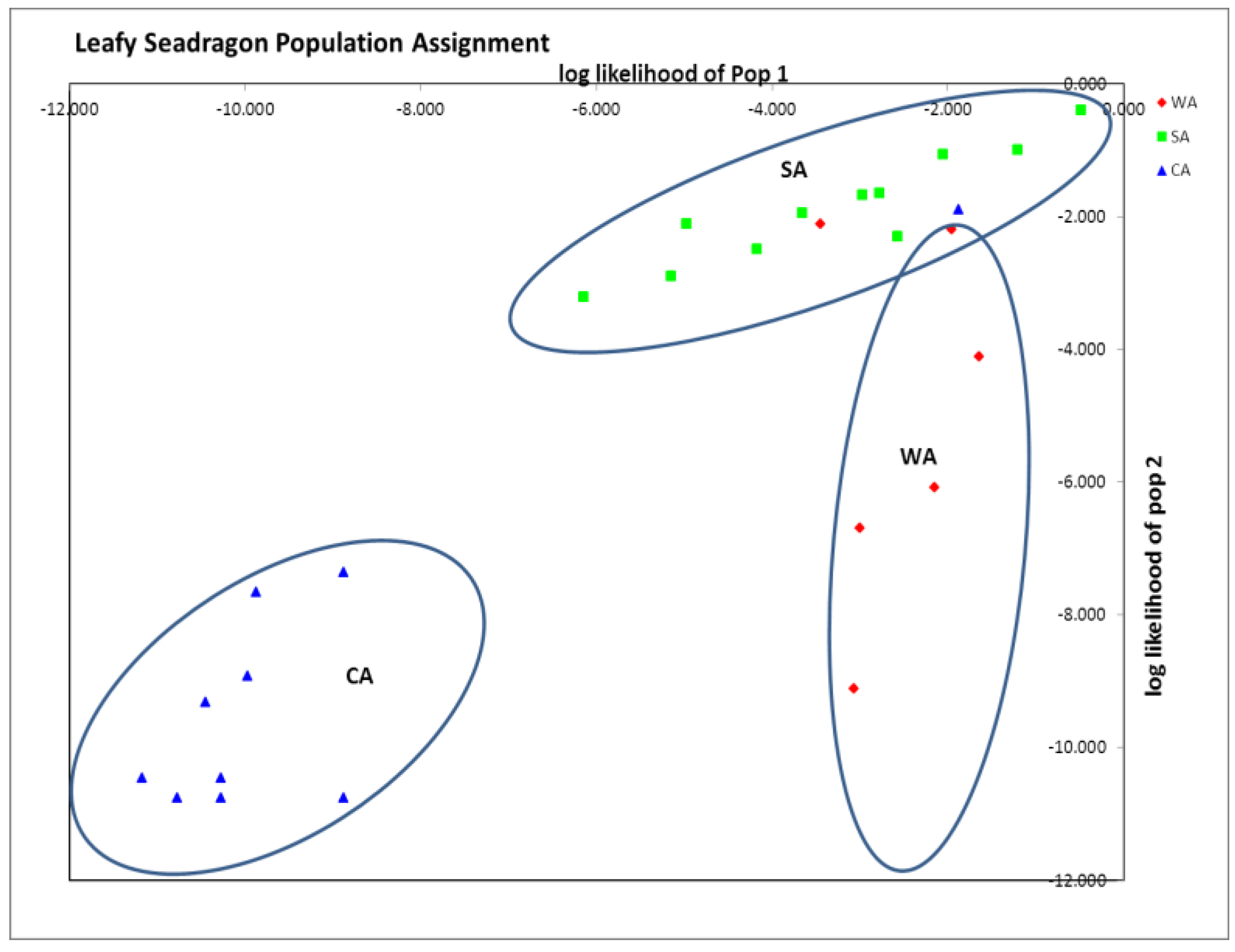
Table 3). STRUCTURE analysis run by testing K = 1 to 10 populations, resulted in the most probable number of distinct populations being one (K with the smallest posterior likelihood or Ln (Pd). Finally GenAlEx population assignment suggested three distinct clusters (96% assignment to population of origin), with only three animals mis-assigning (6%), one from CA and two from WA to SA (
Figure 1). In addition, private alleles were found within all three groups: WA (SH2, SH4, and SH7), SA (SH2, SH4 and SH20) and CA (SH1, SH2 and SH20) (
Table 4). Based on the genetic distances and population assignment tests, three distinct groups seem most probable, even though STRUCTURE suggested one.
Figure 1.
GenAlEx assignment plot showing distinct clustering of all three sampled groups. 96% assigned to the population of origin. Note assignment of 1 captive animals (CA) animals and 2 Western Australia (WA) animals assigned within Southern Australia (SA). Axes are log likelihoods of population assignment.
Table 3.
Nei’s Distance pairwise comparisons above the diagonal and Fst pairwise comparisons below the diagonal for all populations, Western Australia (WA), Southern Australia (SA), and captive animals (CA).
Table 3.
Nei’s Distance pairwise comparisons above the diagonal and Fst pairwise comparisons below the diagonal for all populations, Western Australia (WA), Southern Australia (SA), and captive animals (CA).
| WA | SA | CA |
|---|
| WA | - | 0.170 | 0.377 |
| SA | 0.225 | - | 0.349 |
| CA | 0.212 | 0.188 | - |
Table 4.
Allele size (BP = base pair) of the seven variable microsatellite loci and frequency within Western Australia (WA), Southern Australia (SA) and captive animals (CA). Bold numbers indicate private alleles.
Table 4.
Allele size (BP = base pair) of the seven variable microsatellite loci and frequency within Western Australia (WA), Southern Australia (SA) and captive animals (CA). Bold numbers indicate private alleles.
| Locus | BP size | WA | SA | CA |
|---|
| SH1 | 101 | 0.000 | 0.000 | 0.667 |
| 103 | 0.000 | 0.000 | 0.333 |
| SH2 | 108 | 0.000 | 0.045 | 0.000 |
| 114 | 0.000 | 0.000 | 0.050 |
| 117 | 0.083 | 0.000 | 0.000 |
| 120 | 0.667 | 0.636 | 0.550 |
| 123 | 0.250 | 0.318 | 0.400 |
| SH4 | 196 | 0.000 | 0.056 | 0.000 |
| 198 | 0.100 | 0.389 | 0.167 |
| 200 | 0.100 | 0.389 | 0.000 |
| 206 | 0.400 | 0.000 | 0.000 |
| 208 | 0.400 | 0.056 | 0.333 |
| 210 | 0.000 | 0.111 | 0.500 |
| SH7 | 190 | 0.100 | 0.500 | 0.500 |
| 192 | 0.500 | 0.500 | 0.500 |
| 194 | 0.200 | 0.000 | 0.000 |
| 196 | 0.200 | 0.000 | 0.000 |
| SH15 | 127 | 0.000 | 0.167 | 0.167 |
| 129 | 1.000 | 0.833 | 0.833 |
| SH20 | 213 | 0.000 | 0.000 | 0.111 |
| 222 | 0.500 | 0.429 | 0.278 |
| 225 | 0.100 | 0.000 | 0.611 |
| 228 | 0.000 | 0.071 | 0.000 |
| 231 | 0.400 | 0.500 | 0.000 |
Although all three groups were distinct, there was more genetic similarity between CA and SA than between CA and WA, as indicated by smaller pairwise F
ST and Nei’s D (
Table 3). This result is expected as the only distributor of leafy seadragons to the public aquarium industry, Pang Quong, collects from southern Australian waters [
23]. Thus, this similarity between CA and SA is not surprising, but the population clustering of CA from WA and SA was striking, suggesting that the CA group was genetically distinct from the wild animals (
Figure 1).
The high percentage of population assignments to population of origin and genetic structuring reported here could be due to the high degree of relatedness within the sampled populations. Results of MLRELATE analysis reported relatively high percentage of first order relatedness (Parent-offspring, full-sibling, and half-sibling) within all groups: 40% within WA, 47% within SA, and was 51% within CA. Relatedness between groups was smaller with 28% first order relatives between SA and CA, 7% between CA and WA, and 18% between SA and WA. The high degree of relatedness found within the CA group is not surprising as these animals were cohorts from only a few males collected by Pang Quong in 2000 and 2001. However the degree of relatedness within the wild animals (WA and SA) is surprising. This could be due to the low dispersal of related individuals as a planktonic dispersal phase is missing because the male broods the eggs until the juveniles hatch [
2,
7]. Dispersal of related individuals may also be limited because leafy seadragons are thought to be weak swimmers as they lack a caudal fin. In line with this, acoustic tracking of nine adults reported relatively small movement patterns with home ranges averaging only five hectares [
7].
We acknowledge our sample sizes are small, we have few locations and the loci employed have relatively low diversity. However, Hale, Burg, and Steeves [
24] reported, based on real and simulated populations with sample sizes ranging between 5–100, that an N as low as 5 captured over 90% of the variability in allele frequency and expected heterozygosity within several different taxa (one insect, one mammal, and two birds). They concluded that sampling more than 25 individuals provided little benefit in assessing genetic diversity within a population or genetic structure among populations [
24]. The sample sizes used for this analysis per population are small and less than 25 (six in WA, 11 in SA and 11 in CA), they may be large enough to capture significant diversity and structure, perhaps 90%. Consequently we believe the population parameters reported here are valid, but we also acknowledge that more research needs to be done to measure diversity and structure within seadragons using larger sample sizes over a greater portion of the range.
Results from this study suggest that seadragons have relatively low levels of genetic diversity and locally have high levels of relatedness and population structure. Due to population parameters, such as low levels of dispersal, small home ranges, and high population structuring, seadragons are thought to be vulnerable to local extinctions through pollution, habitat loss, and overharvest [
2,
7]. The Australian government has relatively strict regulations on the harvest of seadragons, allowing little take by collectors [
9,
20]. The most obvious threats to seadragons today are habitat degradation, loss in quality and quantity of habitat, and harassment by recreational divers [
2,
3,
7]. The loss of habitat is most severe near major urban centers, where pollution from discharge of storm water and treated sewage leading to eutrophication and increased sedimentation is considered a primary threat to wild populations [
3]. The threat to the greater seadragon population may be lessened by the occurrence of seadragons at sites distant from urban areas within the seadragon’s range, provided that these areas are biologically connected through movement or dispersal. However, since seadragon dispersal is likely to be limited, as the population structure suggested here, the size and scope of disturbed areas may profoundly affect and enhance the long-term population fragmentation of seadragons.


