Article

Contrasting Patterns of Phytoplankton Assemblages in Two Coastal Ecosystems in Relation to Environmental Factors (Corsica, NW Mediterranean Sea)

1
UMR 6134 Sciences for Environment, UMS 3514 Stella-Mare, CNRS University of Corsica, BP 52, 20250 Corte, France
2
MARE Center, Laboratory of Oceanology, University of Liège, Sart Tilman B6c, 4000 Liege, Belgium
3
STARESO, BP 33, 20260 Calvi, France
*
Author to whom correspondence should be addressed.
Diversity 2014, 6(2), 296-322; https://doi.org/10.3390/d6020296
Submission received: 18 December 2013 / Revised: 18 March 2014 / Accepted: 27 March 2014 / Published: 15 April 2014

Abstract

:
Corsica Island is a sub-basin of the Northwestern Mediterranean Sea, with hydrological features typical of both oligotrophic systems and eutrophic coastal zones. Phytoplankton assemblages in two coastal ecosystems of Corsica (the deep Bay of Calvi and the shallow littoral of Bastia) show contrasting patterns over a one-year cycle. In order to determine what drives these variations, seasonal changes in littoral phytoplankton are considered together with environmental parameters. Our methodology combined a survey of the physico-chemical structure of the subsurface water with a characterization of the phytoplankton community structure. Sampling provided a detailed record of the seasonal changes and successions that occur in these two areas. Results showed that the two sampled stations presented different phytoplankton abundance and distribution patterns, notably during the winter–spring bloom period. Successions in pico-, nano-, and microphytoplankton communities appeared mainly driven by differences in the ability to acquire nutrients, and in community-specific growth rates. Phytoplankton structure and dynamics are discussed in relation to available data on the Northwestern Mediterranean Sea. These results confirm that integrated monitoring of coastal areas is a requisite for gaining a proper understanding of marine ecosystems.

1. Introduction

The Mediterranean Sea (MS) is a semi-enclosed sea with a narrow continental shelf. The combined effects of low precipitation, relatively little river inflow of freshwater and strong evaporation produce a water balance deficit, resulting in high salinity and high temperatures [1]. With its low nutrient availability, the MS is ranked as an oligotrophic-to-ultraoligotrophic system [2]. These characteristics, added to the division of the Western Mediterranean Basin (WMB) into several sub-basins or seas, themselves separated by channels (e.g., Corsica channel), have an important influence on the currents and also on biotic and abiotic water mass parameters [3]. The structure and succession of phytoplankton assemblages are primarily controlled by hydrodynamics and are dependent on nutrient availability, light, temperature, weather conditions, and grazing pressure [4,5].
In the WMB, the vertical structure of the water column shows strong seasonality, characterized by alternating periods of mixing and stratification. This fluctuation generates major changes in the average irradiance experienced by phytoplankton and in nutrient concentrations, modulating phytoplankton dynamics in terms of both community structure and productivity. Phytoplankton blooms occur in winter–spring, when the surface waters begin to stabilize [6,7,8] and occasionally in autumn if wind events and lower surface-water temperatures combine to trigger a thermocline breakdown [9,10,11,12]. Large-size, high-growth-rate diatoms are generally found during these periods (e.g., Chaetoceros sp., Skeletonema sp., Thalassiosira sp. [7,13,14]). While this seasonal pattern of spring bloom and autumn bloom is found throughout the MS, it occurs in different shades, according to coastal ecosystem study sites (Table 1). Recent studies in marine littoral ecosystems highlight a strong heterogeneity of phytoplankton distribution at WMB scale, with high biomass concentrations in some areas (≥3 µg·L−1; [12,15,16,17,18,19]). These differences would be required of strong regional specificities that are expressed in terms of: diversity, relative abundance of species, size class, as well as seasonal succession. Variability of phytoplankton assemblages was explained by (i) the availability of nutrients; (ii) the variation of light; and (iii) mixing conditions [20]. The distribution of species within these assemblages is dependent on the degree of stability and nutrient concentrations [21,22,23,24]. Nutrient inputs can be of natural origin (e.g., rainfall, hydrodynamics; [8,22,25,26]) or anthropogenic origin [27,28].
The phytoplankton is considered a key water quality element for coastal ecosystems in many studies and is the only planktonic element referred to in the Water Framework Directive (WFD). Scientists are working on establishing fast, robust, and reproducible WFD indices to enable environmental managers to assess the quality of their water masses [29]. This simplification hinges on pinpointing the functional dynamics and specific characteristics of the coastal areas studied. Our study is part of this research framework.
Table 1. A non-exhaustive inventory of phytoplankton variation in coastal ecosystems (NW Mediterranean Sea).
Study sitesReferencesStudy periodsPeriods of high biomassDominant taxonomic groups
Catalan coast (Spain)[7]WinterFebruary/March- Diatoms (Chaetoceros sp., Detonula pumila)
Banyuls-sur-Mer (France)[30]Annual cycleFebruary- Diatoms (Skeletonema costatum)Cryptophytes;
April/May- Diatoms (Chaetoceros sp., Nitzschia sp., Rhizolenia delicatula)
Autumn- Diatoms
[14]Annual cycleMarch/April - Diatoms (Chaetoceros sp., Pseudo-nitzschia calliantha, Rhizosolenia sp.), Dinoflagellates (Prorocentrum sp., Protoperidinium sp.);
Summer- Diatoms (Leptocylindrus sp.), Dinoflagellates (Ceratium sp., Gyrodinium sp., Gymnodinium sp., Heterocapsa sp.), Cyanobacteria (Synechococcus sp., ProChlorococcus sp.)
Marseilles (France)[13]Annual cycleFebruary - Diatoms (Skeletonema costatum, Chaetoceros sp., Rhizosolenia stolterfothii);
March/May - Diatoms (Skeletonema costatum, Chaetoceros curvisetus, Lauderia annulata);
Autumn- Diatoms (Skeletonema costatum, Leptocylindrus danicus, Thalassionema nitzschioides, Thalassiothrix frauenfeldii)
[31] Summer- Diatoms, Cryptophytes, large Dinoflagellates
Toulon (France)[15]Annual cycleFebruary/April - Diatoms (Cyclotella sp., Navicula sp.; Licmophora gracilis, Coscinodiscus sp.);
June - Dinoflagellates (Prorocentrum compressum, Gymnodinium sp.);
Autumn- Diatoms (Navicula sp., Coscinodiscus sp., Chaetoceros sp., Cylindrotheca closterium, Cyclotella sp.)
Villefranche-sur-Mer (France)[20]Annual cycleMarch/April- Prymnesiophyceae, Chrysophyceae
November- Diatoms
[32]May - Dinoflagellates (Ceratium furca, Prorocentrum micans, Prorocentrum sp.);
August/September - Diatoms (Thalassionema frauenfeldii), Dictyochophyceae (Dictyocha fibula);
[33]October/November - Diatoms (Chaetoceros sp.);
Summer/Autumn- Diatoms (Dactyliosolen fragilissimus, Leptocylindrus danicus, L. minimus)
Naples (Italy)[34]Annual cycleMay/June - Diatoms (Cylindrotheca closterium, Chaetoceros compressus, Nitzschia longissima);
October- Dinoflagellates, Dictyochophyceae (Emiliana huxleyi);
Winter- Dictyochophyceae (Emiliana huxleyi)
[9]AutumnNovember-Diatoms (Thalassiosira sp., Chaetoceros sp.)
[35]Annual cycleWinter/spring - Diatoms (Chaetoceros compressus, C. didymus, Pseudo-nitzschia delicatissima, Thalassionema bacillaris)
Summer - Diatoms (Skeletonema pseudocostatum, Chaetoceros tenuissimus, C. socialis) Dinoflagellates (Heterocapsa niei, Prorocentrum triestinum)
Autumn- Diatoms (Thalassiosira rotula, Pseudonitzschia delicatissima, Cylindrotheca closterium, Skeletonema menzelii, Dactyliosolen phuketensis, Pseudo-nitzschia multistriata, Leptocylindrus minimus), Dictyochophyceae
Phytoplankton dynamics are complex in coastal areas, relative of offshore areas in Mediterranean Sea. These studies are essential to understand phytoplankton community structure and dynamics, and the influence of environmental factors in the marine littoral ecosystems. Phytoplankton distribution can show high local variability, notably spatial changes even within a season [18]. Despite extensive research on phytoplankton structure and dynamics in the MS, seasonal changes in phytoplankton community are not as well defined in marine littoral ecosystems.
The study area, Corsica Island, is the third largest island in the WMB, with 1,047 km of coastline that is unaffected by strong anthropogenic perturbation and pollution. The topography of the submerged part presents strong vertical asymmetry (Figure 1, [36]). The west coast of Corsica is characterized by a narrow continental shelf and a succession of clearly-marked canyons, creating an area located more than 2,500 m deep. The east coast has a sandy plain with a gentle slope emerging into shallow areas. The 200 m isobath is far from the shore, and depths seldom exceed 500 m, resulting in a fairly straight coast (Figure 1). Corsica Island, from its geographical position, is in a “crossroads” climate, subject to a Mediterranean climate with summer aridness, high brightness, and uneven rainfall, especially in spring when precipitation is frequently sudden and abundant. Winds are all directed towards the island, the most important being southwesterly and northwesterly winds.
Figure 1. Location of Corsica Island, representation of the vertical asymmetry in bathymetric profile (according to French Navy’s Hydrographic and Oceanographic Department (SHOM) map, Western Mediterranean), and maps of the study areas giving station locations: S1, Bay of Calvi ; S2, littoral of Bastia, 1 km offshore and S3, littoral of Bastia, near the coast.
Diversity 06 00296 g001
The distribution of streams and lagoons is also conditioned by the morphology of the island, localized to the main lagoons on the east coast (e.g., Biguglia; Figure 1). The shallow lagoon of Biguglia (Corsica, Western Mediterranean Sea; Figure 1) is a confined ecosystem disturbed by a growing eutrophication, documented since the 1980s [37,38,39]. Its watershed lies to the southwest of the city of Bastia and covers an area of 180 km2 that includes four towns, with a population of approximately 35,000 in winter and around twice that number in summer. For the past four decades, human settlement and associated activities (particularly tourism, agriculture, and industrial activities) have been rapidly increasing around the lagoon [37,39]. They currently pose substantial threats to the water quality and the ecological equilibrium of the lagoon and surrounding marine ecosystem.
This study set out to characterize patterns of phytoplankton assemblages in two coastal ecosystems (east and west coast of Corsica Island) over one year using microscopy and pigment analysis. These two coastal ecosystems differ in terms of oceanographic conditions (frontal structure with significant depths, west coast and sandy plains with depth not exceeding 500 m and nearly a lagoon environment, east coast; Figure 1) and environmental conditions (climate forcing, physical conditions, and nutrient availability). Data on the spatio-temporal distribution of phytoplankton assemblages around Corsica remain scarce. Only in the area of the Bay of Calvi have a few studies on phytoplankton been investigated [8,21,40]. These earlier studies have helped improve knowledge on the spatio-temporal dynamics of phytoplankton assemblages in coastal areas with regional and local specificities.

2. Materials and Methods

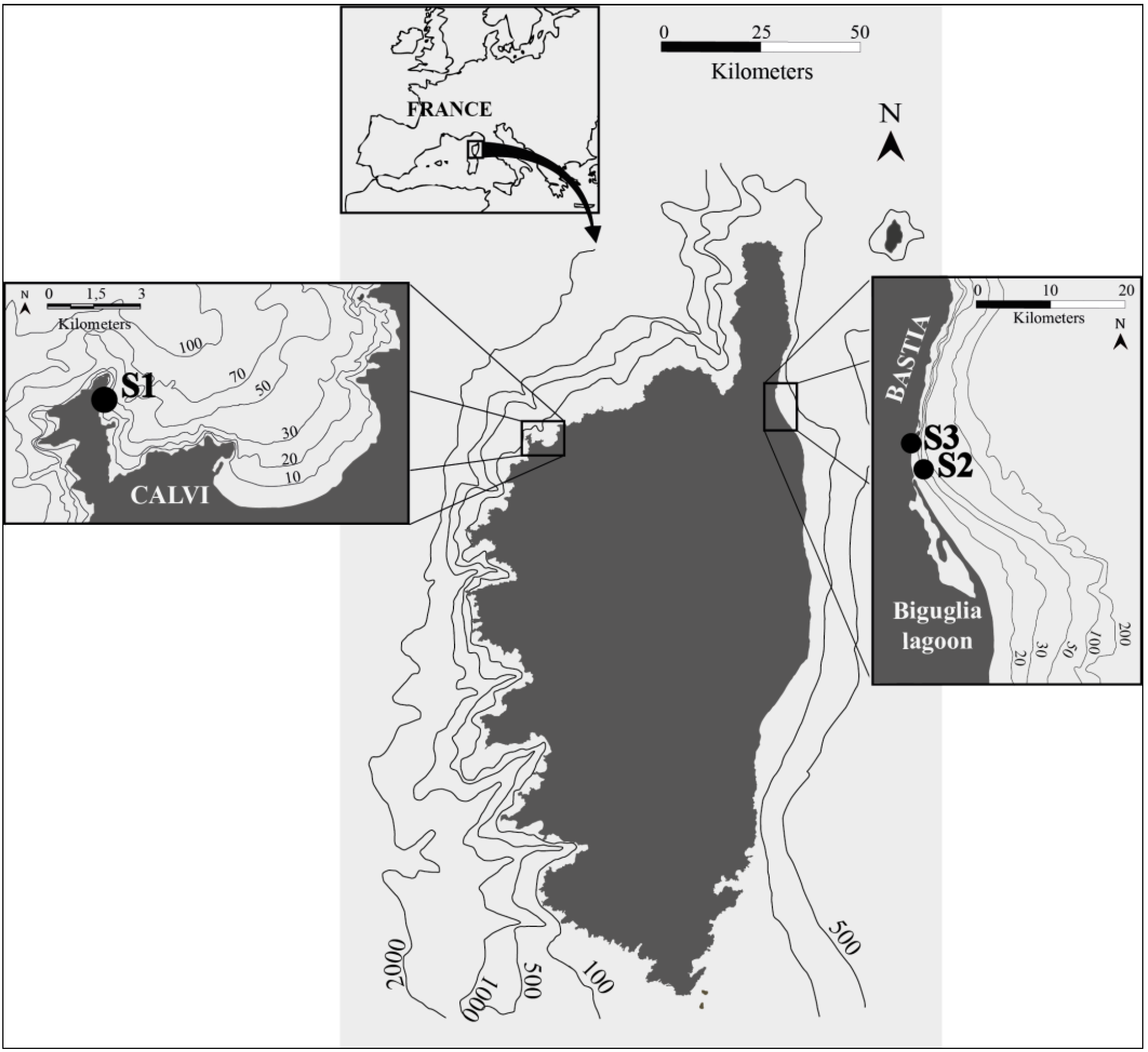
2.1. Sampling Strategy

We chose two stations, one on each coast in Corsica, to compare two coastal ecosystems (Figure 1). The first station is located in the Bay of Calvi, with a low-runoff system opened to the north, which has a narrow continental shelf with a steep canyon (S1, 42°34′50′′N, 08°43′28′′E) and is representative of the area (Bay of Calvi; see [8]), and the second station is located in Bastia, 1 km offshore, with a 20 m depth where the bottom is made of fine sand (S2, 42°38′12′′N, 09°27′15′′E, Figure 1). Near the Bastia sampling station is the widest wet zone of Corsica, Biguglia.
The sampling strategy was the same at both stations (S1 and S2), with monthly sampling during an annual cycle in 2010. Beker et al. [41,42] demonstrated that sampling frequency for studies on phytoplankton dynamics in coastal areas needs to be about a sample every 15 days to capture sudden changes in phytoplankton populations. It is for this reason that, in the Bastia area, where to our knowledge phytoplankton dynamics have not yet been studied, we increased the sampling frequency. The sampling strategy consisted in weekly samplings for five months (January to May) at another station in Bastia, near the coast (S3, 42°40′53′′N, 09°26′51′′E) in order to accurately track in-station phytoplankton dynamics during this period of strongest change in annual variation. Water samples for all analyses were collected from the subsurface between 7:00 a.m. and 8:30 a.m. (local time) at all stations.

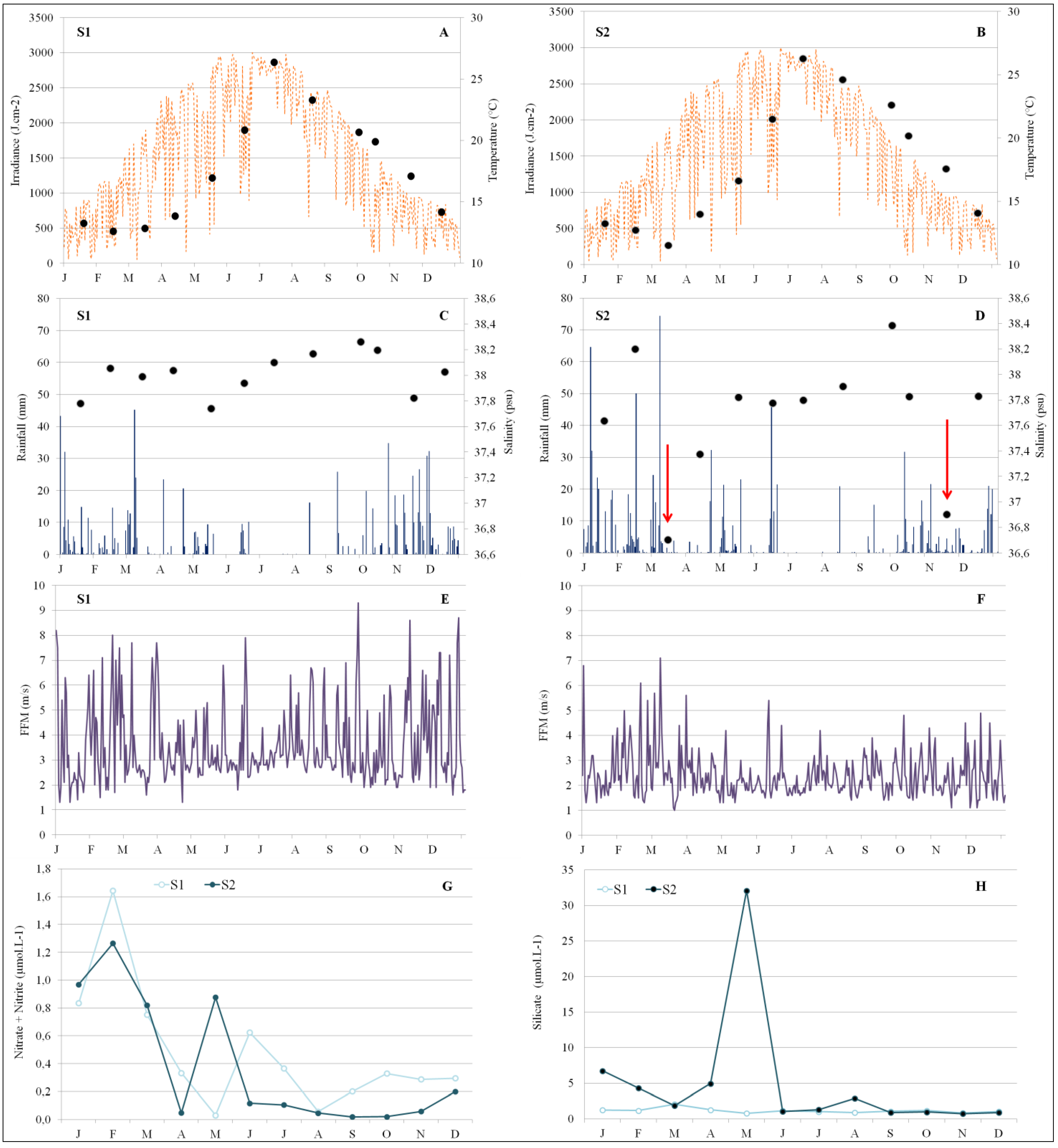
2.2. Physico-Chemical Measurements

Temperature and salinity were measured at each sampling station in the subsurface (±1 m), using two multiparameter probes (Seabird SBE19 and YSI EMS, 6600 V2-2). Meteorological data for 2010 (mean daily irradiance in J·cm−2; daily mean wind velocity in m·s−1 and direction; daily rainfall precipitation in mm) came from Météo-France data recorded at the weather stations located in the Calvi and Bastia airports.
As ammonia is a minor component in our marine environment [8], dissolved inorganic nitrogen concentration was expressed as DIN = Nitrate (NO3) + Nitrite (NO2). Dissolved inorganic phosphorus analyses were not performed for instrumental reasons.

2.3. Phytoplankton Analysis

In order to identify and quantify the phytoplankton samples, 50 L of water was filtered through a silk Apstein 20 µm-screen plankton net, and 100 mL was recovered and fixed with 2.5% formaldehyde solution. All samples were stored at room temperature, in the dark, until analysis. Using an inverted microscope, we examined each sample using the Utermöhl method [43,44]. Numeration at 200× and 400× magnification was carried out on diametric tapes, or on the total chamber surface, depending on species size and abundance [45]. When possible, 400 cells were counted to ensure that the error in estimation of cellular abundance remains within the limits of ±10% [46].
For pigment analysis, 1 L of water was collected and prefiltered through a 200 μm mesh screen to remove mesozooplankton. Water samples were filtered on 25 mm Whatman GF/F glass fiber filters. The filters were frozen (−80 °C) and analyzed by High Performance Liquid Chromatography (HPLC). Samples were extracted in methanol using sonication [47]. Pigment extracts were analyzed by HPLC (Waters Alliance 2695, Waters Corporation: Milford, MA, USA) according to the technique of Zapata et al. [48].
This study used the pigments as size-class markers of phototroph groups [49]. The biomass proportion associated with each size class is defined according to the method described in Claustre [50], and completed by Vidussi et al. [51] (for a detailed description of this pigment index, see [51]).

2.4. Zooplankton Analysis

The mesozooplankton samples were collected monthly using a standard 200 µm mesh-size wp2 net at the S1 (Calvi) and S2 (Bastia) stations. The trawl sampled between 0 and 5 m of the sea subsurface at an average speed of 2 km·h−1, during 20 min for each sample. Water volume filtered was 188 m3. Before transferring the samples from the collector to the jar, the net was washed to collect all plankton trapped in the mesh. The samples were then reduced to a volume of 200 mL and fixed in 2.5% formalin. Mesozooplankton biovolume was measured after 24 h of sedimentation in graduated cylinders. The results are expressed in mL·m−3.

2.5. Data Analysis

Given the low sample size and the large number of variables composing the phytoplankton assemblages, similarity and ordination methods were used to compare samples between both sites (S1, Calvi on the west coast and S2, Bastia on the east coast of Corsica Island) and across the 12 sampled months (January to December). These methods are particularly suited for multivariate analysis of ecological data as they do neither assume a priory structure among samples (e.g., grouping of samples among sites) nor normality of the probability distribution of data. Data was log-transformed and similarity matrices between samples using the Bray–Curtis similarity index were computed prior to analysis.
Winter–spring bloom dynamic of phytoplankton assemblages at Bastia: S2 vs. S3—Prior spatio-temporal analysis of phytoplankton assemblages (using pigment composition as a proxy), we evaluated the effect of sampling frequency of phytoplankton assemblages on their composition at Bastia, on the east coast of Corsica. Differences in composition of phytoplankton assemblages sampled at S2 and S3 were described using clustering and ordination methods in order to identify eventual grouping of samples. A non-metric multi-dimensional scaling ordination (MDS) was applied in conjunction with a cluster analysis based on the unweighted pair group method with arithmetic mean. Investigated using the same methods as described below for the comparison between S1 Calvi and S2 Bastia. The variability of phytoplankton assemblages was formally examined between sites (S2 and S3) using a PERmutational Multivariate ANalysis Of VAriance (PERMANOVA), which relies on the analysis of similarities between samples [52,53].
Spatio-temporal variation of phytoplankton assemblages: S1 vs. S2—The variability of phytoplankton assemblages was investigated either using the composition of pigments composition (ng L−1; issued from the HPLC) or of phytoplankton groups (cell L−1; identified manually by microscopy). The similarity of phytoplankton assemblages of sites S1 (west coast) and S2 (east coast) and across the 12 months sampled, were first described using a MDS applied in conjunction with a cluster analysis, as described above for the comparison between S2 and S3. When ecologically meaningful clusters could be identified among samples, they were used as grouping factors for the subsequent statistical analyses.
The variability of phytoplankton assemblages across sites was formally examined using a PERMANOVA. p-values for the PERMANOVAs were obtained, for each term of the model, with unrestricted permutations of raw data and Type III sums of squares. Unconstrained clusters, MDS and PERMANOVA were performed with the PRIMER software version 6.1.13 [54] and the PERMANOVA add-on [55].
Abiotic drivers of phytoplankton assemblages in Bastia and Calvi—Pair-wise plots and spearman rank-correlations were first conducted to estimate the association between the measured chemical seawater parameters (temperature, salinity, DIN, silicate), meteorological data (wind, rain), and the principal classes of phytoplankton and the corresponding specific marker pigments.
Distance based Multivariate Regression Trees (MRT) were then performed for both sites (S1 and S2) to define the habitat type (environmental parameters and their threshold values) associated with the different phytoplankton assemblage types isolated by each clusters. MRT is a constrained clustering method, reliable for analyzing community data without making any a priory assumption about the form of the relationship between the species matrix (in our study case, the classes of phytoplankton) and their environment [56]. The MRT were computed using a Bray–Curtis dissimilarity index.
The environmental preferences of classes of phytoplankton were then identified using an indicator species analysis based on the classification of assemblages from the MRT analysis. The indicator species analysis was performed using a “point biserial” correlation coefficient of association, corrected for unequal group sizes, which is the abundance-based Pearson’s phi coefficient of association [57]. This correlation index accounts for the ecological preference of species) among the set of clusters isolated by the MRTs. p-values for each indicator species were obtained using random permutation. Analyses were performed using classes of phytoplankton identified by microscopy.
MRT and indicator species were performed using the GPL software R version 3.0.2 [58] and respectively the “mvpart” [59] and “indicspecies” packages [60].
Succession between phytoplankton and zooplankton—Cross-correlations were performed between zooplankton bio-volumes and Chl a, and fucoxanthin, the specific marker of diatoms, to investigate the succession of zoo- and phytoplankton.

3. Results

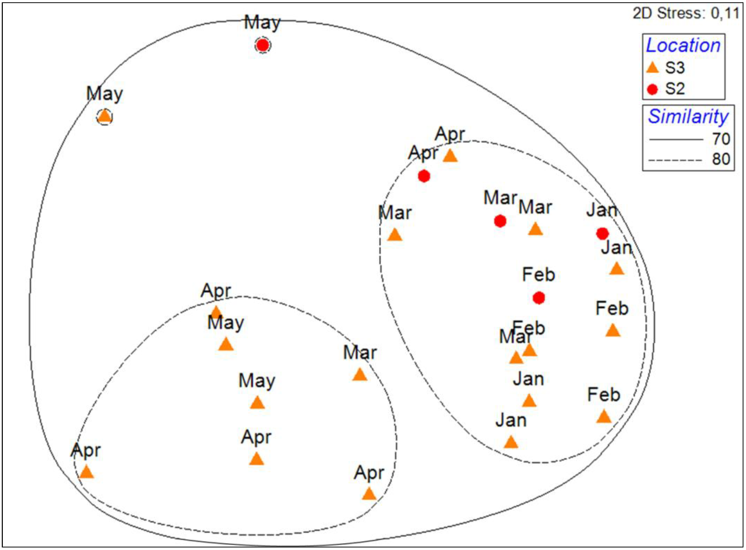
3.1. Winter–Spring Bloom Dynamic of the Phytoplankton Assemblages at Bastia

In Bastia, phytoplankton assemblages showed similar patterns for the two sampling stations (S2 and S3; Figure 1) during the five months period from January to May 2010 (Figure 2). No clear separation was visible between samples taken at S2 and S3 (Figure 2) on the multi-dimensional scaling ordination. However, some samples taken at S3 during March, April and May seemed to show different pigment compositions than those taken at S2 (Figure 2).
Figure 2. MDS of pigment composition of phytoplancton assemblages in S2 (Bastia, sampling station located 1 km offshore, in red) and S3 (Bastia, near the coast, in orange) coupled to a cluster analysis. Solid and dashed lines represent the principal clusters identified at respectively a 70 and 80% Bray Curtis similarity.
Diversity 06 00296 g002
Two samples in May appeared also to have different pigment compositions. However, PERMANOVAshowed no significant differences between the pigment composition of phytoplankton assemblages of S2 sampled at a monthly frequency and S3 sampled at a weekly frequency (df = 1, MS: 349.71, Pseudo-F: 2.005, p-values: 0.1167).

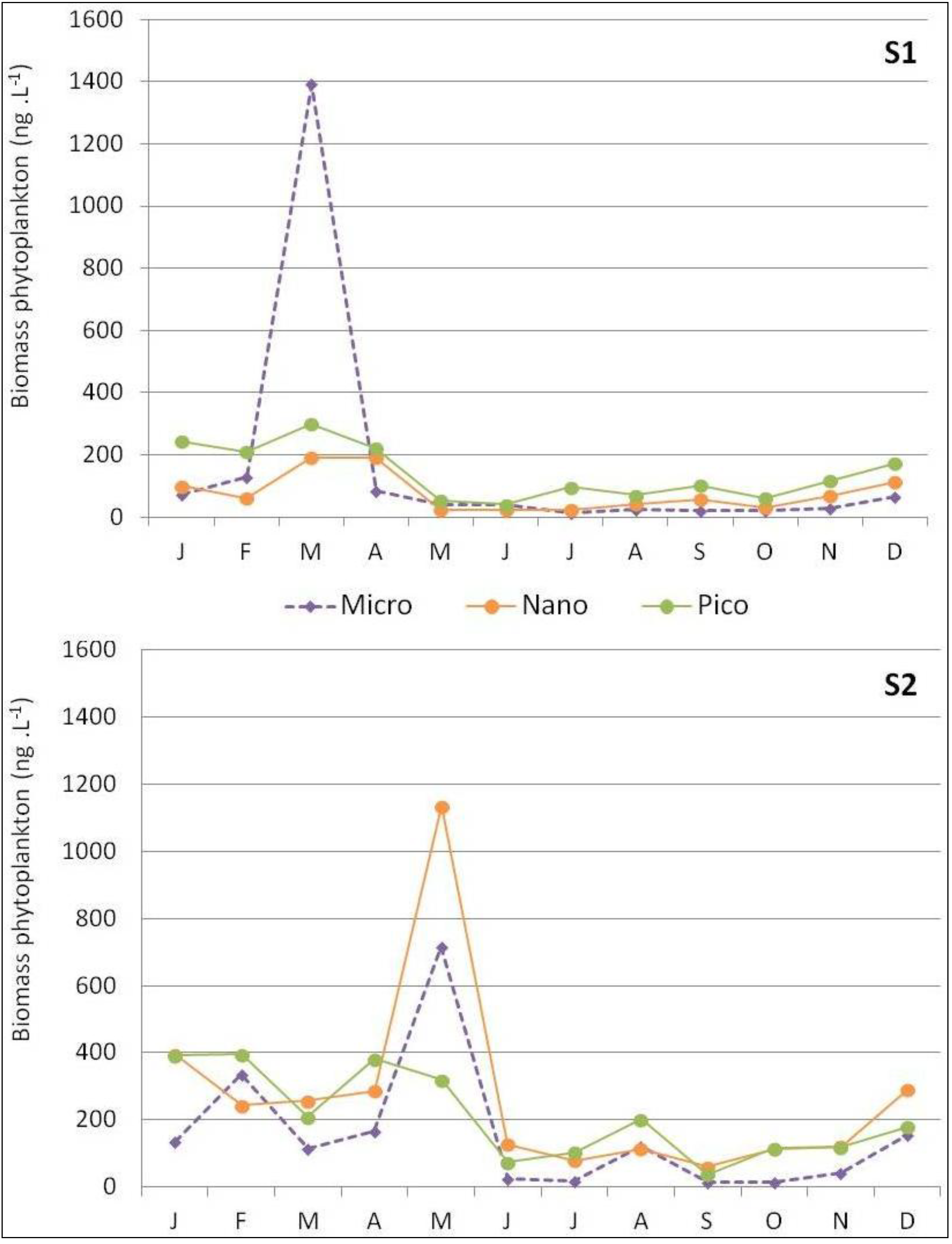
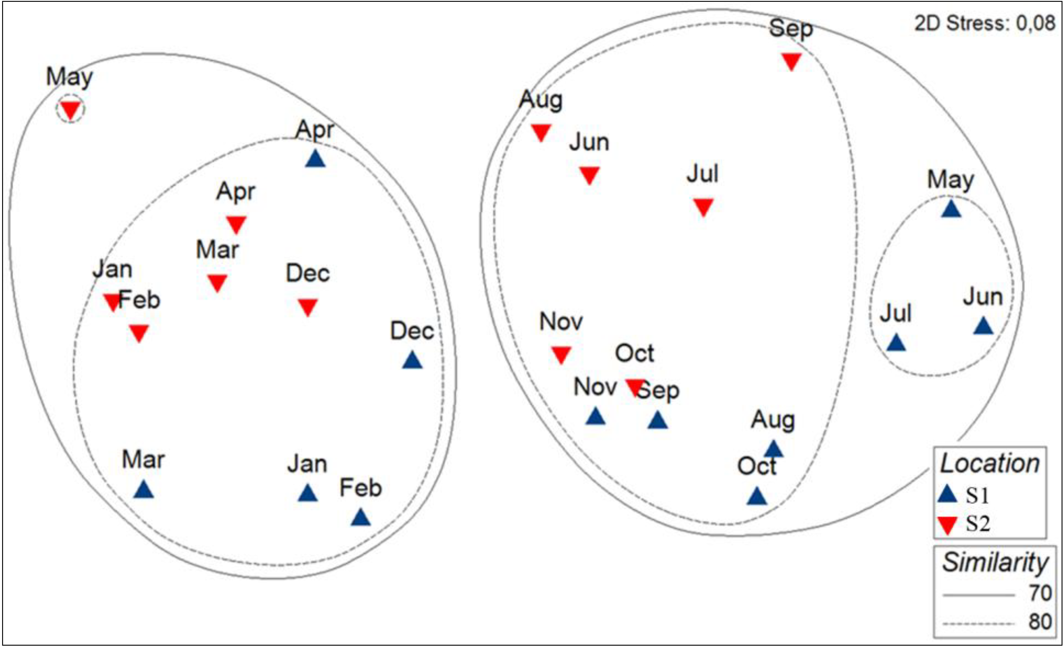
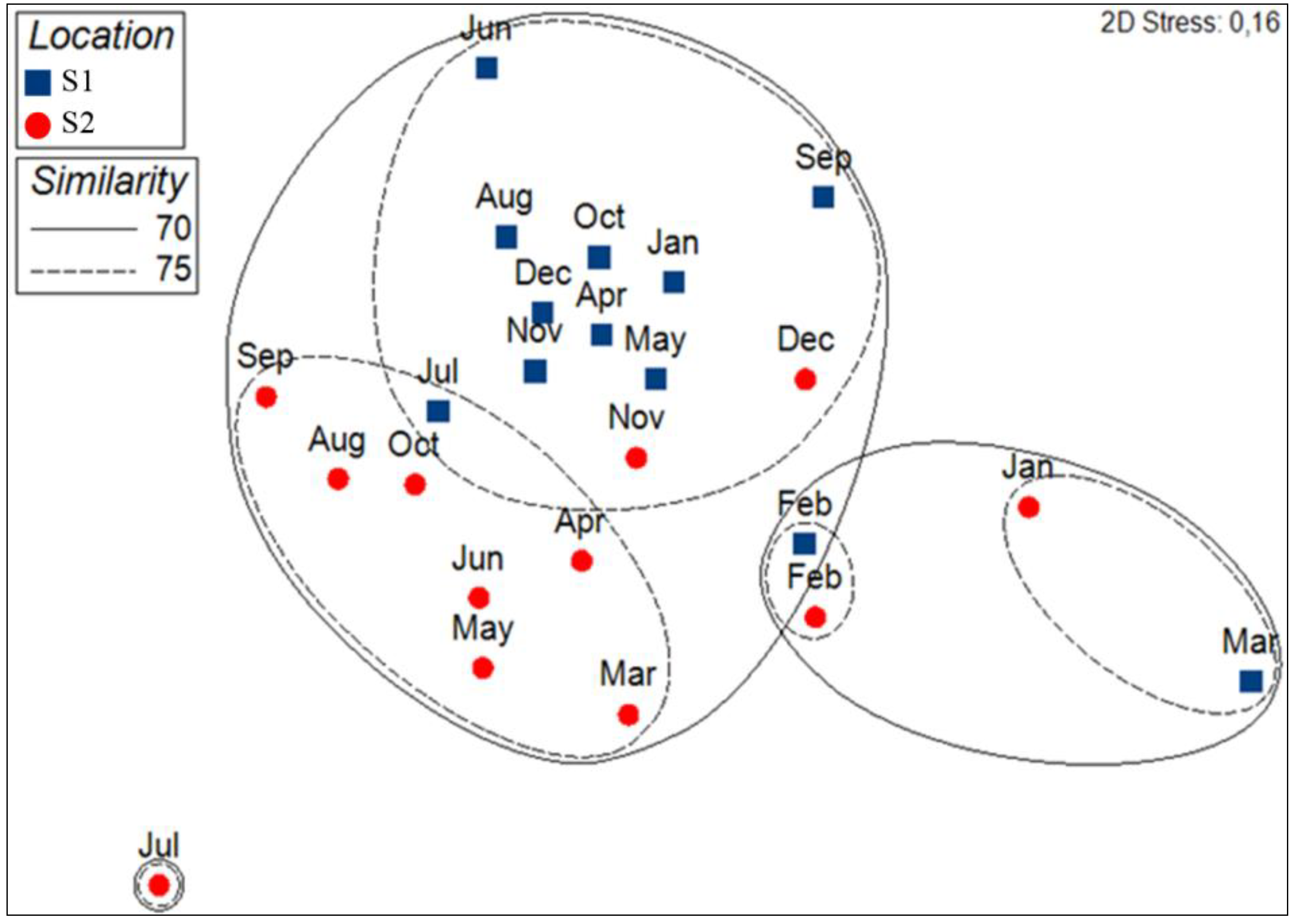
3.2. Spatio-Temporal Variation of Phytoplankton Assemblages at Bastia and Calvi

In S1 (Calvi station), subsurface Chl a concentrations varied from 86.9 to 1,815.2 ng·L−1 (Figure 3). Subsurface Chl a concentrations were only high in March (1,815.2 ng·L−1). Chl a concentrations were low during the other months (monthly average except March: 290.2 ng·L−1), but increased slightly from November. In S2 (Bastia station), subsurface Chl a concentrations varied from 100.3 to 2,143.4 ng·L−1 during the annual cycle (Figure 3). Chl a concentrations were highly correlated between S2 and S1 with a time lag of two months (R2 = 0.882; Confidence Interval CI = 0.566). However, compared to S1, two distinct periods were observed: Chl a concentrations were high between January and May (up to 2,143.4 ng·L−1 in May) and low during the rest of the year (June to December; monthly average of 291.0 ng·L−1), and increasing from October (Figure 3). The spatio-temporal variability of Chl a concentrations were associated with characteristic compositions on each station.
Figure 3. Spatio-temporal subsurface diversity of phytoplankton assemblages and Chl a variation, during 2010, at S1 and S2 stations (Ø no dominant taxonomic groups).
Diversity 06 00296 g003
Picophytoplankton biomass dominated in S1 in subsurface waters (with an annual mean of 50% and a biomass of 140.0 ng·L−1; Figure 4), associated with zeaxanthin (Figure 5; 29.3% of all pigments, data not shown). High microphytoplankton concentrations, at 74% proportion or 1,391.1 ng·L−1 (Figure 4), were only detected in March, and were associated with high fucoxanthin concentrations (Figure 5; 59% proportion of all pigments, data not shown).
Figure 4. Spatio-temporal variability of biomass size classes for micro-, nano-, and picophytoplankton according to the equation of Vidussi et al. [40] at S1 and S2 stations.
Diversity 06 00296 g004
In S2, biomass was dominated by a wide range of size classes during the first period (January to May; Figure 4). Nanophytoplankton biomass dominated in subsurface waters (with an annual mean of 43% and a biomass of 268.6 ng·L−1; Figure 4), associated with 19’-hexanoyloxyfucoxanthin (Figure 5; 32.1% proportion of all pigments, data not shown). Microphytoplankton were only found in February and in May (34% or 334.4 ng·L−1 and 33% or 714.3 ng·L−1, respectively; Figure 4), and marked by high fucoxanthin concentrations in February (Figure 5; 27% proportion of all pigments, data not shown). High microphytoplankton concentrations, at 74% proportion or 1,391.1 ng·L−1 (Figure 4), were only detected in March, and were associated with high fucoxanthin concentrations (Figure 5; 59% proportion of all pigments, data not shown). In S2, biomass was dominated by a wide range of size classes during the first period (January to May; Figure 4). Nanophytoplankton biomass dominated in subsurface waters (with an annual mean of 43% and a biomass of 268.6 ng·L−1; Figure 4), associated with 19-hexanoyloxyfucoxanthin (Figure 5; 32.1% proportion of all pigments, data not shown). Microphytoplankton were only found in February and in May (34% or 334.4 ng·L−1 and 33% or 714.3 ng·L−1, respectively; Figure 4), and marked by high fucoxanthin concentrations in February (Figure 5; 27% proportion of all pigments, data not shown).
Figure 5. Spatio-temporal evolution of the principal classes of phytoplankton and the corresponding specific marker pigments at S1 and S2.
Diversity 06 00296 g005
MDS revealed two principal groups, differentiating mainly the pigment assemblages of samples taken in winter/spring from those taken in summer/autumn at similarity threshold of 66% (Figure 6). It is to notice that the winter/spring cluster consisted of samples from January to April and December at S1, whereas it consisted of samples from January to May and December at S2.
Figure 6. MDS of pigment composition of phytoplancton assemblages of S1 (Calvi, in blue) and S2 (Bastia, in red) coupled to a cluster analysis. Solid and dashed lines represent the principal clusters identified at, respectively, a 70% and 80% Bray–Curtis similarity.
Diversity 06 00296 g006
The PERMANOVA confirmed the significant differences of pigment composition between the winter/spring and the summer/autumn clusters (Table 2 and Table 3). Significant differences for the pair-wise test of terms of the interaction term of factor site (i.e., S1 and S2) and season (i.e., winter/spring and summer/autumn; Table 2 and Table 3).
Table 2. Two-way crossed PERMANOVA of pigment composition between sites (S1 and S2) and seasons (winter/spring and summer/autum). Degree of freedom (df), mean square (MS), pseudo-F statistic and permutational p-values are given for each term of the model.
Source of VariationdfMSPseudo-Fp-values
Site11130.16.88070.0034
Season14768.929.0360.0001
Site × Season1214.811.30790.2487
Residuals20164.24
Total23
Table 3. Pair-wise tests for the interaction term between sites and seasons, with comparisons between sites S1 and S2 within the winter/spring and the summer/autumn terms of season.
S1 (Calvi) vs. S2 (Bastia)
Seasontp-values
winter/spring2.02660.0051
summer/autumn2.08840.0033
Microscopy observations confirmed that the early spring bloom in each station (March in S1 and February/May in S2; Figure 4) could be largely attributed to the presence of large phytoplankton cells consisting mainly of Chromophytes dominated by Chaetoceros sp. Diatomophyceae (up to 776 × 103 cell·L−1 in S1 in March, and up to 275 × 103 cell·L−1 in S2 in February; Figure 3). Microscopy also revealed the occurrence of Licmophora sp. blooming in winter–spring in S1 (up to 149 × 103 cell·L−1 in February) and Thalassionema sp. in S2 (128 × 103 cell·L−1; Figure 3). Dinophyceae were mainly represented, in July for S1, and during May to August for S2. The diversity of genera encountered was greater in S2, with Ceratium furca (in spring and in summer), Prorocentrum sp., and Protoperidinium sp. (in spring). Dinophysis sp. was present occasionally in S2. Prymnesiophyceae were also found at various concentrations. Numerous colonial cells of Phaeocystis sp. were present all year long but especially in April/May in S1 (Figure 3 and Figure 4). In S2, Syracosphaera sp. was encountered in spring and summer, while Rhabdosphaera sp. was found mostly in summer and autumn.
The diatoms Coscinodiscus sp. in S1 in November and Leptocylindrus sp. and Chaetoceros sp. in S2 in November were found to be associated with upper water column freshening events (lagoon inputs and runoff; see rainfall, Section 3.3. at the two stations). Most of the pico- and nanophytoplanktonic cells appeared as rounded forms, lacking discriminating morphological characters, making it impossible to identify them.
According to the MDS plots, phytoplankton assemblages are distinct in January and February in S2, and February and March in S1 from samples taken during the other months of the year (Figure 7). A relative grouping of the rest of the samples between S1 and S2 was visible at a similarity threshold of 74.78% (Figure 7). PERMANOVA showed significant differences in phytoplankton assemblage composition between S1 and S2 (df = 1, MS: 1,075, Pseudo-F: 2.939, p-values: 0.0172).
Figure 7. MDS of phytoplankton assemblages of Calvi (S1, in blue) and Bastia (S2, in red) coupled to a cluster analysis. Solid and dashed lines represent the principal clusters identified at respectively a 70% and 75% Bray Curtis similarity.
Diversity 06 00296 g007

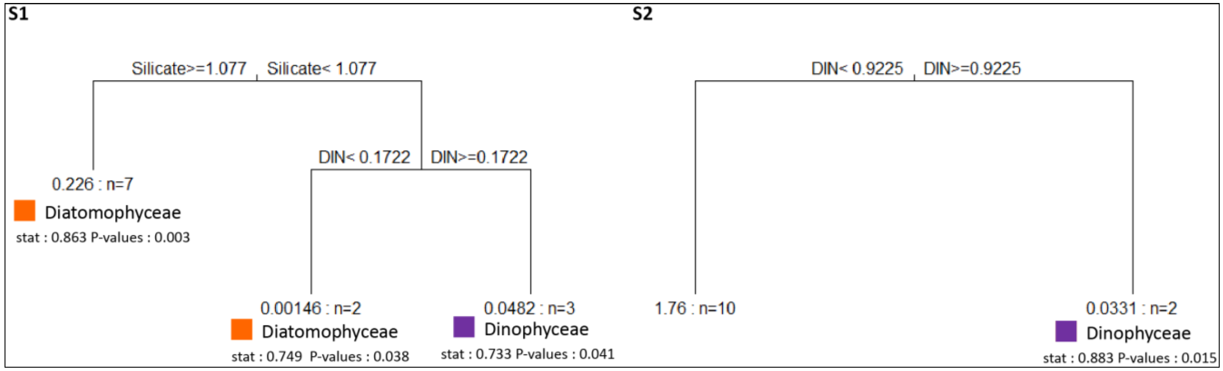
3.3. Abiotic Drivers of Phytoplankton Assemblages

The in situ temperature probed at the subsurface followed a typical seasonal pattern with a gradual increase during summer, and was highly correlated between S1 and S2 (R2 = 0.986; p-values < 0.0001), ranging from 12.4 °C to 26.3 °C in S1, and 12.6 °C to 26.4 °C in S2 (Figure 8A,B).
Figure 8. Spatio-temporal variations of subsurface environmental parameters during 2010 in the two stations (S1 and S2); (A) and (B): subsurface temperature (°C; dots; right scale) and mean daily irradiance (J·cm−2; line; left scale); (C) and (D): weekly rainfall (mm; bars; left scale) and subsurface salinity (psu; lines; right scale); (E) and (F): daily mean wind velocity; (G): Dissolved inorganic nitrogen concentration, nitrite + nitrate; (H): silicate.
Diversity 06 00296 g008
S1 subsurface salinity remained fairly unchanged all year long (37.7–38.4; Figure 8C). In S2, low salinity revealed that two freshening events occurred in March and in November, when subsurface salinities fell to 36.7 and 36.9, respectively (Figure 8D), explaining the absence of correlation between salinity on S1 and S2 (R2 = 0.559; p-values: 0.0627).
Rainfall over 2010 was significantly correlated between the two coasts, with an annual average of 74.9 in S1 and 86.2 mm in S2 (R2 = 0.545; p-values: 0.0457). In S1, major rainfall events were recorded between September and December (429.8 mm against 278.1 mm in S2), while in S2, precipitations were heavier during the winter-spring period (January to June, 734.1 mm against 451.7 mm in S1; Figure 8C,D).
Wind episodes were more numerous and more intense in Calvi compared to Bastia (1.0 to 7.3 m·s−1 in S2 vs. 1.3 to 9.3 m·s−1 in S1), explaining the absence of correlation between wind episodes at S1 and S2 (R2 = 0.024; p-values: 0.9397). Winds were southwesterly almost all year round in S1 (windspeeds up to 13.7 m·s−1 in February), while in S2, winds switched between southwesterly and southeasterly (windspeeds up to 10.9 m s−1 in February; Figure 8E,F).
DIN and silicate concentrations showed seasonal variation, with the highest values recorded during winter-spring in both stations (Figure 8G,H). In S1 (Calvi), silicate concentrations were highest in March (2.07 µmol·L−1; Figure 3H), while subsurface nitrate concentrations ranged from low (<0.05 μmol·L−1) to 1.34 μmol·L−1 in February. In S2 (Bastia), subsurface dissolved inorganic nitrogen concentrations ranged from very low (<0.05 μmol·L−1) up to 1.26 μmol·L−1 in June. Subsurface silicate concentrations were high in S2 during winter–spring, up to 32.09 µmol·L−1 in May, and similar at S1 from June to December, except August, at 2.90 µmol·L−1. These differences explain that seasonal variations in silicate (R2 = 0.244; p-values: 0.4435) and in DIN were thus uncorrelated between S1 and S2 (R2 = 0.545; p-values: 0.0706).
In S1, for dominant taxonomic groups and abiotic drivers, pair-plots and correlation analyses (spearman rank-correlation) revealed that significant correlations were observed for Diatomophyceae with Dinophyceae, Dinophyceae with temperature and Prymnesiophyceae with salinity (Figure 9, p < 0.01) and more generally a very high significant correlation between Chl a and silicate (Figure 9, p < 0.001, R2 = 0.9231).
In S2, statistical analyses (Pair-plots and correlation analyses) revealed more correlation between phytoplankton assemblages and environmental variables (Figure 9). Diatomophyceae are significantly correlated with Dinophyceae, Prymnesiophyceae, Cyanophyceae concerning dominant taxonomic groups (Figure 9, p < 0.01). Diatomophyceae and Dinophyceae seem driven by temperature (Figure 9, p < 0.01). Chl a was significantly and positively correlated with silicate and DIN (Figure 9) and temperature was also significantly and positively correlated with DIN and rainfall (Figure 9).
At S1, MRT analysis revealed that among the environmental variables, silicate and DIN concentrations were the primary drivers of phytoplankton assemblages (Figure 10). At S1, the indicator analysis showed that Diatomophyceae were the characteristic taxonomic group of environments with high silicate concentrations (i.e., ≥1.077 µmol) and DIN concentrations below 0.172 µmol. Dinophyceae were typical of environments with DIN concentrations above 0.172 µmol (Figure 10).
At S2, MRT revealed that DIN was the primary abiotic driver of phytoplankton assemblages (Figure 10). At S2, Diatomophyceae were representative of DIN concentrations below 0.922 µmol (Figure 10).
Figure 9. Pair-plots and spearman rank-correlation for dominant taxonomic groups and environmental parameters. Significant correlations are framed in red.
Diversity 06 00296 g009
Figure 10. Multivariate Regression Tree (MRT) and corresponding indicator classes of phytoplankton for S1 and S2. Composition of phytoplankton assemblages are the response variable and environmental variables the constraint of the MRT. Mean densities of phytoplankton assemblages and number of cases are displayed at the end of each leave. Above each split of the trees is indicated the abiotic variable and its threshold value on which the split is based. The tree explains 0.58% of the variance of phytoplankton assemblages at S1 and 0.59% at S2. The depth of the tree following each split is proportional to the variance explained by the split. Stat: correlation index translating the ecological preference of some classes of phytoplankton for particular environmental conditions.
Diversity 06 00296 g010

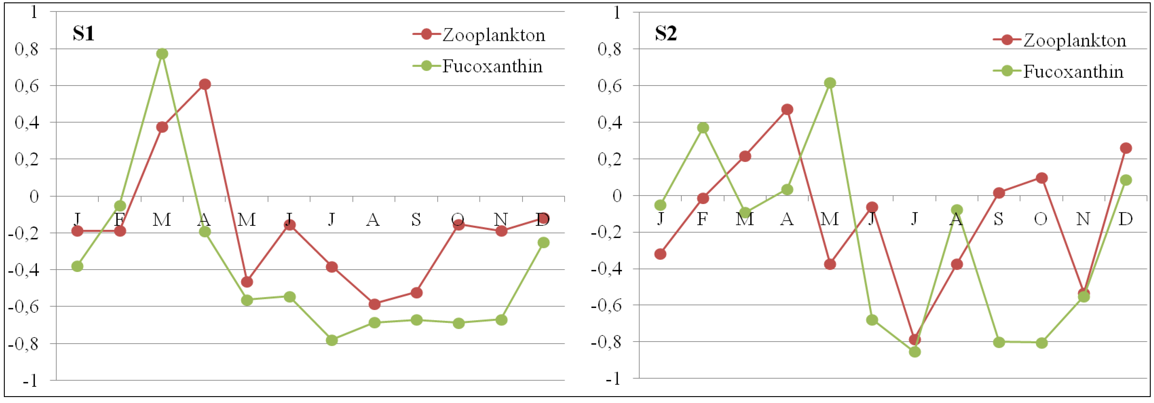
3.4. Zooplankton Variation

The zooplankton cycle, expressed from biovolumes, also showed seasonal fluctuations in S1 (0.05 to 0.82 mL·m−3) and S2 (0.02 to 0.48 mL·m−3). Peak values were recorded in April at both stations (Figure 11). Zooplankton communities succeeded phytoplankton assemblages. At S1, zooplankton biovolume was significantly correlated to total Chl a and to fucoxanthin, the diatom-specific marker, at a one month time lag (Chl a: R2 = 0.893, CI = 0.566; fucoxanthin: R2 = 0.911, CI = 0.566; Figure 11). The correlation was less clear for S2 (Chl a: R2 = 0.619, CI = 0.566; fucoxanthin: R2 = 0.716, CI = 0.566) due to sampling frequency. Results of Chl a at Bastia sampled at a weekly frequency (S3) showed a phytoplankton bloom in April, which was not visible at the monthly sampled station S2.
Figure 11. Relative data on zooplanktonic biovolume and fucoxanthin (specific marker pigment of diatoms) in S1 and S2 stations during the annual cycle.
Diversity 06 00296 g011

4. Discussion-Conclusions

This study provides new data on the spatio-temporal variability of phytoplankton in coastal ecosystems in the Northwestern Mediterranean Sea. Margalef’s theory of ecological succession in phytoplankton can be completely applied to coastal ecosystems ([61], the “Margalef’s mandala” commented by Wyatt [62]). Phytoplankton assemblages in the MS are characterized by three annual succession phases that drive the pioneer winter populations to a final state by increasing the maturity of the system. The data interpretation of this study was separated into the intra-annual variations of phytoplankton assemblages, i.e., (i) winter–spring bloom period; (ii) late-bloom and summer periods; and (iii) autumn period. Monthly sampling, as we did, provided instantaneous pictures that do not allow comprehensive analyses, and interpretations of the phytoplankton dynamic, owing to the time-scale of adaptive strategies (from seconds for individual physiological traits to days for structural changes of the community composition). “The issue of what constitutes a bloom is more than simply a biomass issue” [63] and includes in particular temporal considerations regarding frequency and/or periodicity of occurrence [62] that are not directly available in the present work.
In the MS, the first phase generally occurs in winter (February–March) prior to the thermal stratification that is assumed to be the prerequisite for the “classical” spring bloom of temperate regions [64]. The biomass increase is recorded over the majority of the water column, generally involving large-sized high-growth-rate diatoms (e.g., Chaetoceros sp., Skeletonema sp., Thalassiosira sp.; [13,14,65]). Indeed, the winter bloom has been defined as the unifying feature for phytoplankton in the Northwestern MS [66], where it has been recorded all along the coast (Table 1). A similar situation was found during this research campaign in our stations (S1 and S2). Chl a concentrations in the subsurface water, during the winter–spring period, presented high maximum values. These data are consistent with published variations for surface waters in winter–spring [6,7,18,19,35,67,68]. However, when we compared S1 and S2 stations over the first five months of the year (period involving the strongest variations), winter–spring conditions and phytoplankton dynamics clearly showed different patterns. In Calvi (S1; west coast of Corsica), peak phytoplankton biomass was recorded in March, and diatoms dominated (Chaetoceros decipiens, C. didymus, C. peruvianus, C. simplex, C. socialis). Indeed, DIN:DSi ratio exceeds the 1:1 ratio suggested to represent the average utilization of diatoms [69], which is observed in Calvi. In Bastia (S2; east coast of Corsica), Chl a concentrations were high throughout the winter–spring period (January and May, monthly average: 1,077.4 ng·L−1). Diatom abundance was high in March (Chaetoceros decipiens, C. didymus, C. socialis, Thalassiosira eccentrica), whereas nanophytoplankton dominated in other months. The peak biomass in May was represented by dinoflagellates (Prorocentrum micans, P. minimum, P. compressum, and Ceratium furca). Given that diatoms are typical of well-mixed, nutrient-rich environments [63,70], our results showed that coastal waters of Bastia (S2) were not always as well mixed as would be expected for Calvi and the Northwestern Mediterranean littoral zone [71,72]. Indeed, at S1, the winter–spring period corresponded to vertical thermocline movement under the influence of local wind-driven upwelling events, and the injection of nutrients through across-thermocline mixing induced by the Liguro–Provençal front [73,74]. In February, nutrient concentrations are highest, while the nutrient levels show a strong decrease in April from the previous month, combined with the spring phytoplankton bloom. These data are consistent with published phytoplankton variations at Calvi [8,21,75]. At S2, the winter–spring period also corresponded to vertical thermocline movement and the injection of nutrients induced here during this period by rainfall, runoff of rivers (Golo river) and the proximity of an eutrophic environment (Biguglia Lagoon).
These local specificities could explain the high concentration of Chl a during a five-month period and the low abundance of diatoms. Phytoplankton assemblages are selected by their tolerance to surrounding biotic and abiotic pressures (e.g., turbulence, pollution, and predation) and by their ability to compete for resources [76]. Diatoms are very sensitive to changing environmental conditions [77]. The Biguglia Lagoon is a confined ecosystem with increasing eutrophication since 1980 [37,38]. Inputs from brackish lagoon waters during winter–spring, induced by strong rainfall events (Figure 3A,B), could explain why diatoms have not dominated in this coastal area and why dinoflagellates and nanophytoplankton, which cope better with changing environments, are found in higher numbers. As a primary producer, diatoms are key organisms in the water ecosystem [77]. Moreover, they are beneficial to the higher trophic chain. Indeed, at our two stations, zooplanktonic herbivores appeared after the phytoplanktonic spring bloom. For the first phase, these results for the winter–spring period are consistent with earlier reports on coastal ecosystems in many Northwestern MS areas (Table 1). On the Catalan coastline, with a deep basin near the frontal system (Catalan and North Balearic fronts), Estrada et al. [7] found similar phytoplankton groups for the same study period compared to Calvi (S1), which are also subjected to a frontal system (the Liguro-Provençal front; Table 1). The permanent frontal zone is a highly dynamic area, where a complex network of the divergences brings nutrients from deep water into the euphotic zone, thereby enhancing new phytoplankton production [7,8]. Areas with shallow basins show different ecological successions of phytoplankton assemblages, with high Chl a concentrations represented by large diatoms (March/April) and dinoflagellates (April/May), as in the Bastia station (S2) and in Banyuls-sur-Mer ([14], Table 1). The most striking impact was brought about by upper water column freshening as a result of river runoff (Golo River and Bevinco River via the lagoon of Biguglia), and to some extent local rainfall, which both freshened the surface water—changing its buoyancy and stability—and introduced a fairly substantial amount of nutrients. These physical instabilities led to seasonal and vertical shifts in the supply and distribution of nutrients, particularly in shallow littoral waters [14,30].
The second phase or late-bloom and summer periods were characterized by a decrease in nutrient and Chl a concentrations in both stations, consistent with published variations for oligotrophic surface waters for this period [12,51,57,78]. Chl a biomass was essentially dominated by pico- and nanophytoplankton, which contributed 75% of total Chl a in Calvi and 81% of the annual cycle in Bastia. Li [79] showed that as a rule, a drop in Chl a concentration drives an increase in pico- and nanophytoplankton. This profile is similar to reports from Marty et al. [32], and Bel-Hassen et al. [80], in the Western MS, where relative contributions for these size groups were about 85%. A dinoflagellate bloom involving Prorocentrum and Ceratium genera, and cyanobacteria, occurred in Bastia. In the same case as Banyuls-sur-Mer, small dinoflagellates and cyanobacteria were observed ([14], Table 1). However, others areas of Northwestern MS have a similar assemblage structure but with slightly more small diatoms (e.g., Naples, Table 1). The summer phase is characterized by strong thermal stratification, which leads to a 50-m-deep thermocline with low-level nutrients and low biological activity [32,81,82]. Here, nutrient concentrations (nitrate and silicate) in subsurface waters gradually deplete and virtually disappear as the season progresses, directly due to photosynthetic activity and the thermocline preventing nutrient upflow from deep water to the surface.
During the third phase, in autumn, phytoplankton diversity remained low, probably because less-competitive species were eliminated by the persistent post-summer oligotrophic conditions [24]. The dominance of picophytoplankton confirms the principle that small species are more competitive and abundant in nutrient-depleted conditions [83], and when salinity is higher (August and September at S2). Thermocline breakdown together with the effects of wind events and lower surface-water temperatures can sometimes lead to phytoplankton blooms [9,10,11,12]. In Calvi and Bastia, in October, Chl a concentrations increased slowly and large diatoms appeared. However, Chl a concentrations were higher at S2, where enrichment resulted both from autumn rainfalls and exchanges with the lagoon environment. An ecologically important nutrient enrichment may also take place in autumn with the leaching of the soil during rainfall events [14,84]. An extreme enrichment, occurring after intensive rainfalls in late winter (Figure 8A,B), was rapidly exploited by a single potentially toxic species that dominated numerically, leading to a biomass peak, a drop in diversity, and potential HAB (Harmful Algal Blooms) formation [84]. In shallow littoral waters, the unpredictability of physical disturbances and nutrient supplies associated with the generally accepted idea that waters are always well-mixed, may explain that seasonal changes in phytoplankton community are not as well defined as “offshore.” Consequently, the causes driving these shifts remain somewhat uncertain or to be unraveled: storms, rainfall, river runoff, or advective transports, being most often evoked [14,30,85].
For coastal ecosystems, seasonal and stochastic fluctuations of environmental factors [86] define large and stereotyped environmental windows (The “Margalef’s mandala” commented on by Wyatt [62]) that are said to select and frame the composition and abundance of phytoplankton assembalges [87]. Comparing the structure of assemblages, driven by anthropogenic nutrient inputs to the structure of assemblages, following natural succession can provide vital insights into the rules governing phytoplankton community and assemblage responses to changes in environmental conditions. In order to achieve this, the HPLC technique proved to be useful for improving the ecological understanding of the phytoplankton assemblages in the study area, a clear relationship between phytoplankton composition (at the level of major taxonomic groups) and anthropogenic pressure was not clearly established in this study. The complexity of life and nutritional strategies [88], even within the same taxonomic group, makes the development of a community composition indicator very difficult. However, we have seen that different hydroclimatic and environmental factors (e.g., rainfall, runoff via Biguglia Lagoon, Liguro–Provençal Front) are an important natural component affecting phytoplankton composition, and this can also hinder the development of composition based metrics [89].
In regard to the requirements to assess the community composition within different policies, especially within the WFD, there is no agreement, yet, in the way it has to be assessed [90,91]. However, in the last WFD intercalibration report, Carletti and Heiskanen [92] have addressed the importance of characterizing the phytoplankton assemblages and the need to link composition to nutrient enrichment and other pressures. On the basis of the investigations conducted, thus far at Corsica Island, the integration of physical and biological data has to be considered a prerequisite for an exhaustive understanding of the marine ecosystem dynamics at these coastal sites. Connections between environmental context and human activities make it difficult to detect and assess marine ecosystems responses, and, for this reason, we suggest that more effort should be devoted to these regional functions, including by promoting continuous monitoring of coastal areas, but also concerning technical equipment and software tools. Different authors (e.g., [93,94]) have addressed the HPLC-CHEMTAX approach—CHEMTAX is a matrix factorization program—as an effective tool for comparative purposes within the WFD perspective. Furthermore, the advance in the latest chromatographic techniques [48] permits a better resolution among pigments, as well as the possibility to discover new marker pigments [95,96,97,98], which helps in the use of pigmentary techniques for the description of the community composition as we have put forward in this study.

Acknowledgments

This study was supported by funding from the French Government and from the Corsican Regional Council. Marie Garrido was financially supported by a grant from the Collectivité Territoriale de Corse and the University of Corsica. We would like to thank all the STARESO team and the University of Liege (Belgium). We also thank Guillaume De Liege and Aurélie Fouquoire from the University of Corsica. The authors are grateful to Francesca Vidussi for providing valuable help on using the taxonomic pigments.

Author Contributions

The work presented here was carried out in collaboration between Marie Garrido, Anne Goffart, Jean-Henri Hecq and Vanina Pasqualini for define the research theme. Anne Goffart and Jean-Henri Hecq designed methods. Equipment and instruments were available for sampling in Calvi station by Pierre Lejeune, Jean-Henri Hecq and Amandine Collignon. Marie Garrid, Vanina Pasqualini and Anne Goffart co-worked on associated data collection for Calvi station and Marie Garrido and Vanina Pasqualini co-worked on associated data collection for Bastia stations. Marie Garrido carried out the laboratory experiments, analyzed the data, interpreted the results and wrote the paper. Marie Garrido and Vanina Pasqualini discussed analyses, interpretation, and presentation. Marie Garrid and Barbara Koeck discussed analyses, interpretation, and presentation for statistical data. Barbara Koeck wrote the part “statistical analyses”. Sylvia Agostini and Bernard Marchand have reviewed and approved the manuscript.

Conflicts of Interest

The authors declare no conflict of interest.

References

  1. Béthoux, J.P.; Gentili, B.; Morin, P.; Nicolas, E.; Pierre, C.; Ruiz-Pino, D. The Mediterranean Sea: A miniature ocean for climatic and environmental studies and a key for the climatic functioning of the North Atlantic. Prog. Oceanogr. 1999, 44, 131–146. [Google Scholar] [CrossRef]
  2. Krom, M.D.; Kress, N.; Brenner, S.; Gordon, L. Phosphorous limitation of primary productivity in the Eastern Mediterranean Sea. Limnol. Oceanogr. 1991, 36, 424–432. [Google Scholar] [CrossRef]
  3. Millot, C. Circulation in the Western Mediterranean Sea. J. Mar. Syst. 1999, 20, 423–442. [Google Scholar] [CrossRef]
  4. Richardson, K.; Beardall, J.; Raven, J.A. Adaptation of unicellular algae to irradiance: An analysis of strategies. New Phytol. 1983, 93, 157–191. [Google Scholar] [CrossRef]
  5. Anderson, A.; Haecky, P.; Hagstroem, A. Effect of temperature and light on the growth of micro, nano and picoplankton: Impact on algal succession. Mar. Biol. 1994, 120, 511–520. [Google Scholar] [CrossRef]
  6. Estrada, M. Phytoplankton assemblages across a NW Mediterranean front: Changes from winter mixing to spring stratification. Oecol. Aquat. 1991, 10, 157–185. [Google Scholar]
  7. Estrada, M.; Varela, R.; Salat, J.; Cruzado, A.; Arias, E. Spatio-temporal variability of the winter phytoplankton distribution across the Catalan and North Balearic fronts (NW Mediterranean). J. Plankton Res. 1999, 21, 1–20. [Google Scholar] [CrossRef]
  8. Goffart, A.; Hecq, J.H.; Legendre, L. Changes in the development of the winter-spring phytoplankton bloom in the Bay of Calvi (NW Mediterranean) over the last two decades: A response to changing climate? Mar. Ecol. Prog. Ser. 2002, 236, 45–60. [Google Scholar] [CrossRef]
  9. Zingone, A.; Casotti, R.; Rivera d’Alcala, M.; Scardi, M.; Marino, D. St Martin’s summer: The case of an autumn phytoplankton bloom in the Gulf of Naples (Mediterranean Sea). J. Plankton Res. 1995, 17, 575–593. [Google Scholar] [CrossRef]
  10. Estrada, M. Primary production in the northwestern Mediterranean. Sci. Mar. 1996, 60, 55–64. [Google Scholar]
  11. Andersen, V.; Prieur, L. One-month study in the open NW Mediterranean Sea (DYNAPROC experiment, May 1995): Overview of the hydrobiogeochemical structures and effects of wind events. Deep-Sea Res. Part I 2000, 47, 397–422. [Google Scholar] [CrossRef]
  12. Vilicic, D.; Bosak, S.; Buric, Z.; Caput-Mihalic, K. Phytoplankton seasonality and composition along the coastal NE Adriatic Sea during the extremely low Po River discharge in 2006. Acta Bot. Croat. 2007, 66, 101–115. [Google Scholar]
  13. Travers, M. Diversité du microplancton du Golfe de Marseille en 1964. Mar. Biol. 1971, 8, 308–343. (In French) [Google Scholar] [CrossRef]
  14. Charles, F.; Lantoine, F.; Brugel, S.; Chrétiennot-Dinet, M.J.; Quiroga, I.; Rivière, B. Seasonal survey of the phytoplankton biomass, composition and production in a littoral NW Mediterranean site, with special emphasis on the picoplanktonic contribution. Est. Coast. Shelf Sci. 2005, 65, 199–212. [Google Scholar] [CrossRef]
  15. Jamet, J.L.; Jean, N.; Bogé, G.; Richard, S.; Jamet, D. Plankton succession and assemblage structure in two neighbouring littoral ecosystems in the north-west Mediterranean Sea. Mar. Freshw. Res. 2005, 56, 69–83. [Google Scholar] [CrossRef]
  16. Polat, S.; Akiz, A.; Olgunoğlu, M.P. Daily variations of coastal phytoplankton assemblages in summer conditions of the northeastern Mediterranean (Bay of İskenderun). Pak. J. Bot. 2005, 37, 715–724. [Google Scholar]
  17. D’Ortenzio, F.; Ribera d’Alcalà, M. On the trophic regimes of the Mediterranean Sea: A satellite analysis. Biogeosciences 2009, 6, 139–148. [Google Scholar] [CrossRef]
  18. Siokou-Frangou, I.; Christaki, U.; Mazzocchi, M.G.; Montresor, M.; Ribera d’Alcala, M.; Vaqué, D.; Zingone, A. Plankton in the open Mediterranean Sea: A review. Biogeosciences 2010, 7, 1543–1586. [Google Scholar] [CrossRef] [Green Version]
  19. Gohin, F. Annual cycles of Chlorophyll-a, non-algal suspended particulate matter and turbidity observed from space and in situ coastal waters. Ocean Sci. 2011, 7, 705–732. [Google Scholar] [CrossRef]
  20. Smayda, T.J.; Reynolds, C.S. Community assembly in marine phytoplankton: Application of recent models to harmful dinoflagellates blooms. J. Plankton Res. 2001, 23, 447–461. [Google Scholar] [CrossRef]
  21. Goffart, A.; Hecq, J.H.; Prieur, L. Contrôle du phytoplancton du bassin Ligure par le front Liguro-Provençal (secteur Corse). Oceanol. Acta 1995, 18, 329–342. (In French) [Google Scholar]
  22. Fouilland, E.; Courties, C.; Descolas-Gros, C. Size-fractionated carboxylase activities during a 32h cycle at 30 m depth in the north-western Mediterranean Sea after an episodic wind event. J. Plankton Res. 2001, 23, 623–632. [Google Scholar] [CrossRef]
  23. Pinazo, C.; Marsaleix, P.; Millet, B.; Estournel, C.; Kondrachoff, V.; Vehil, R. Phytoplankton variability in summer in the Northwestern Mediterranean: Modelling of the wind and freshwater impacts. J. Coast. Res. 2001, 17, 146–161. [Google Scholar]
  24. Spatharis, S.; Tsirtsis, G.; Danielidis, D.B.; Do Chi, T.; Mouillot, D. Effects of pulsed nutrient inputs on phytoplankton assemblage structure and blooms in an enclosed coastal area. Est. Coast. Shelf Sci. 2007, 73, 807–815. [Google Scholar] [CrossRef]
  25. Bustillos-Guzman, J.; Claustre, H.; Marty, J.C. Specific phytoplankton signatures and their relationship to hydrographic conditions in the coastal northwestern Mediterranean Sea. Mar. Ecol. Prog. Ser. 1995, 124, 247–258. [Google Scholar]
  26. Andersen, V.; Nival, P.; Caparroy, P.; Gubanova, A. Zooplankton community during the transition from spring bloom to oligotrophy in the open NW Mediterranean and effects of wind events. 1. Abundance and specific composition. J. Plankton Res. 2001, 23, 227–242. [Google Scholar] [CrossRef]
  27. Vidal, M.; Duarte, C.M. Nutrient accumulation at different supply rates in experimental Mediterranean planktonic communities. Mar. Ecol. Prog. Ser. 2000, 207, 1–11. [Google Scholar]
  28. Béthoux, J.P.; Morin, P.; Ruiz-Pino, D.P. Temporal trends in nutrient ratios: Chemical evidence of Mediterranean ecosystem changes driven by human activity. Deep-Sea Res. Part II 2002, 49, 2007–2016. [Google Scholar] [CrossRef]
  29. Spatharis, S.; Tsirtsis, G. Ecological quality scales based on phytoplankton for the implementation of Water Framework Directive in the Eastern Mediterranean. Ecol. Indic. 2010, 10, 840–847. [Google Scholar] [CrossRef]
  30. Jacques, G. Aspects quantitatifs du phytoplancton de Banyuls sur Mer (Golfe du Lion). III Diatomées et Dinoflagellés de juin 1965 à juin 1968. Vie et Milieu 1968, 20, 91–126. (In French) [Google Scholar]
  31. Thyssen, M.; Beker, B.; Ediger, D.; Yilmaz, D.; Garcia, N.; Denis, M. Phytoplankton distribution during two contrasted summers in a Mediterranean harbour: Combining automated submersible flow cytometry with conventional techniques. Environ. Monit. Assess. 2011, 173, 1–16. [Google Scholar]
  32. Gomez, F.; Gorsky, G. Annual microplankton cycles in Villefranche Bay, Ligurian Sea, NW Mediterranean. J. Plankton Res. 2003, 25, 323–339. [Google Scholar] [CrossRef]
  33. Marty, J.C.; Garcia, N.; Raimbault, P. Phytoplankton dynamics and primary production under late summer conditions in the NW Mediterranean Sea. Deep-Sea Res. Part. I 2008, 55, 1131–1149. [Google Scholar] [CrossRef]
  34. Carrada, G.C.; Hopkins, T.S.; Bonaduce, G.; Ianora, A.; Marino, D.; Modigh, M.; Ribera d’Alcalà, M.; Scotto di Carlo, B. Variability in the hydrographic and biological features of the Gulf of Naples. Mar. Ecol. 1980, 1, 105–120. [Google Scholar] [CrossRef]
  35. Ribera d’Alcalà, M.; Conversano, F.; Corato, F.; Licandro, P.; Mangoni, O.; Marina, D.; Mazzocchi, M.G.; Modigh, M.; Montresor, M.; Nardella, M.; et al. Seasonal patterns in plankton communities in a pluriannual time series at a coastal Mediterranean site (Gulf of Naples): An attempt to discern recurrences and trends. Sci. Mar. 2004, 68, 65–83. [Google Scholar]
  36. Pasqualini, V.; Pergent-Martini, C.; Clabaut, P.; Pergent, G. Mapping of Posidonia oceanica using Aerial photographs and Side Scan Sonar: Application off the Island of Corsica (France). Est. Coast. Shelf Sci. 1998, 47, 359–367. [Google Scholar] [CrossRef]
  37. Mouillot, D.; Titeux, A.; Migon, C.; Sandroni, V.; Frodello, J.P.; Viale, D. Anthropogenic influences on a mediterranean Nature Reserve: Modelling and forecasting. Environ. Model. Assess. 2000, 5, 185–192. [Google Scholar] [CrossRef]
  38. Garrido, M. Structure et fonction des communautés phytoplanctoniques en milieux côtiers marin et lagunaire (Méditerranée–Corse) dans une optique de gestion. Ph.D. Thesis, University of Corsica, Corte, France, University of Liège, Liège, Belgium, 2012. [Google Scholar]
  39. Lafabrie, C.; Garrido, M.; Cecchi, P.; Leboulanger, C.; Gregori, G.; Pasqualini, V.; Pringault, O. Impact of contaminated sediment resuspension on phytoplankton in a Mediterranean lagoon: Functional and structural responses. Est. Coast. Shelf Sci. 2013, 130, 70–80. [Google Scholar] [CrossRef]
  40. Goffart, A. Influence des contraintes hydrodynamiques sur la structure des communautés phytoplanctoniques du bassin Liguro-Provençal (secteur Corse). Ph.D. Thesis, University of Liège, Liège, Belgium, 1992; p. 163. [Google Scholar]
  41. Beker, B.; Romano, J.C.; Arlhac, D. Le suivi de la variabilité des peuplements phytoplanctoniques en milieu marin littoral: Le golf de Marseille en 1996–1997. Océanis 2001, 25, 395–415. (In French) [Google Scholar]
  42. Tréguer, P.; LeCorre, P. Manuel d’analyse des sels nutritifs dans l’eau de mer. Utilisation de l’AutoAnalyser II Technicon, 2nd ed.; University Bretagne Occidentale: Laboratoire de Chimie Marine, Brest, France, 1975; pp. 1–110. (In French) [Google Scholar]
  43. Utermöhl, H. Zur vervollkommnung der quantitativen phytoplanktonmethodik, Mitteilungen der internationalen Vereinigung fur Theoretische and Angewandte. Limnologie 1958, 9, 1–38. (In French) [Google Scholar]
  44. Association Française de Normalisation (AFNOR). Qualité de l'eau—Norme Guide Pour Le Dénombrement Du Phytoplancton Par Microscopie Inversée (Méthode Utermöhl); AFNOR: Saint-Denis, France, 2006; p. 39. (In French) [Google Scholar]
  45. Lund, J.W.G.; Kipling, C.; Le Cren, E.D. The inverted microscope method of estimating algal numbers and the statistical basis of estimations by counting. Hydrobiologia 1958, 11, 143–170. [Google Scholar] [CrossRef]
  46. Uehlinger, V. Etude statistique des méthodes de dénombrement planctonique. Arch. Des Sci. 1964, 17, 11–223. [Google Scholar]
  47. Jeffrey, S.W.; Mantoura, R.F.C.; Bjørnland, T. Data for the identification of 47 key phytoplankton pigments. In Phytoplankton Pigments in Oceanography; Jeffrey, S.W., Mantoura, R.F.C., Wright, S.W., Eds.; UNESCO (United Nations Educational, Scientific and Cultural Organization): Paris, France, 1997; pp. 447–559. [Google Scholar]
  48. Zapata, M.; Rodriguez, F.; Garrido, J.L. Separation of chlorophylls and carotenoids from marine phytoplankton: A new HPLC method using a reversed phase C8 column and pyridine-containing mobile phases. Mar. Ecol. Prog. Ser. 2000, 195, 29–45. [Google Scholar] [CrossRef]
  49. Sieburth, J.M.; Smetacek, V.; Lenz, J. Pelagic ecosystem structure: Heterotrophic compartments of the plankton and their relationship to plankton size fractions. Limnol. Oceanogr. 1978, 23, 1256–1263. [Google Scholar] [CrossRef]
  50. Claustre, H. The trophic status of various oceanic provinces as revealed by phytoplankton pigment signatures. Limnol. Oceanogr. 1994, 39, 1206–1210. [Google Scholar] [CrossRef]
  51. Vidussi, F.; Claustre, H.; Manca, B.B.; Luchetta, A.; Marty, J.C. Phytoplankton pigment distribution in relation to upper thermocline circulation in the eastern Mediterranean Sea during winter. J. Geophys. Res. 2001, 106, 19939–19956. [Google Scholar] [CrossRef]
  52. Anderson, M.J. A new method for non-parametric multivariate analysis of variance. Austral Ecol. 2001, 26, 32–46. [Google Scholar]
  53. Anderson, M.J.; Ter Braak, C.J.F. Permutation tests for multi-factorial analysis of variance. J. Stat. Comput. Simul. 2003, 73, 85–113. [Google Scholar] [CrossRef]
  54. Clarke, K.R.; Gorley, R.N. PRIMER v6: User Manual/Tutorial; PRIMER-E: Plymouth, UK, 2006. [Google Scholar]
  55. Clarke, K.R.; Warwick, R.M. Change in Marine Communities: An Approach to Statistical Analysis and Interpretation; Plymouth Marine Laboratory, PRIMER-E Limited.: Plymouth, UK, 2001; p. 177. [Google Scholar]
  56. De’ath, G. Multivariate Regression Trees: A New Technique for Modeling Species-Environment Relationships. Ecology 2002, 83, 1105–1117. [Google Scholar]
  57. Chytrý, M.; Tichý, L.; Holt, J.; Botta-Dukát, Z. Determination of diagnostic species with statistical fidelity measures. J. Veg. Sci. 2002, 13, 79–90. [Google Scholar] [CrossRef]
  58. R Core Team. R: A Language and Environment for Statistical Computing; R Foundation for Statistical Computing: Vienna, Austria, 2013. [Google Scholar]
  59. De’ath, G. Mvpart: Multivariate Partitioning, R package version 1.6-1; R Foundation for Statistical Computing: Vienna, Austria, 2013. [Google Scholar]
  60. De Cáceres, M.; Legendre, P. Associations between species and groups of sites: Indices and statistical inference. Ecology 2009, 90, 3566–3574. [Google Scholar] [CrossRef]
  61. Margalef, R. Temporal succession and spatial heterogeneity in phytoplankton. Perspect. Mar. Biol. 1958, 323–349. [Google Scholar]
  62. Wyatt, T. Margalef’s mandala and phytoplankton bloom strategies. Deep-Sea Res. Part. II 2014, 101, 32–49. [Google Scholar] [CrossRef]
  63. Smayda, T.J. What is a bloom? A commentary. Limnol. Oceanogr. 1997, 42, 1132–1136. [Google Scholar] [CrossRef]
  64. Sverdrup, H.U. On conditions for the vernal blooming of phytoplankton. J. Cons. Perm. Int. Explor. Mer. 1953, 18, 287–295. [Google Scholar] [CrossRef]
  65. Lévy, M.; Mémery, L.; André, J.M. Simulation of primary production and export fluxes in the Northwestern Mediterranean Sea. J. Mar. Res. 1998, 56, 197–238. [Google Scholar] [CrossRef]
  66. Duarte, C.M.; Agusti, S.; Kennedy, H.; Vaqué, D. The Mediterranean climate as a template for Mediterranean marine ecosystems: The example of the northeast Spanish littoral. Progr. Oceanogr. 1999, 44, 245–270. [Google Scholar] [CrossRef]
  67. Delgado, M.; Latasa, M.; Estrada, M. Variability in the size-fractionated distribution of the phytoplankton across the Catalan front of the north-west Mediterranean. J. Plankton Res. 1992, 14, 753–771. [Google Scholar] [CrossRef]
  68. Mercado, J.M.; Ramirez, T.; Cortés, T.; Sebastian, T.; Vargas-Yaez, M. Seasonal and inter-annual variability of the phytoplankton communities in an upwelling area of the Alboran Sea (SW Mediterranean Sea). Sci. Mar. 2005, 69, 451–465. [Google Scholar]
  69. Brzezinski, M.A. The Si-C-N ratio of marine diatoms-interspecific variability and the effect of some environmental variables. J. Phycol. 1985, 21, 347–357. [Google Scholar] [CrossRef]
  70. Margalef, R. Life-forms of phytoplankton as survival alternatives in an unstable environment. Oceanol. Acta 1978, 1, 493–509. [Google Scholar]
  71. Agawin, N.S.R.; Duarte, C.M.; Agusti, S. Growth and abundance of Synechococcus. sp. in a Mediterranean Bay: Seasonality and relationship with temperature. Mar. Ecol. Prog. Ser. 1998, 170, 45–53. [Google Scholar] [CrossRef]
  72. Agusti, S.; Duarte, C.M. Experimental induction of a large phytoplankton bloom in Antarctic coastal waters. Mar. Ecol. Prog. Ser. 2000, 206, 73–85. [Google Scholar] [CrossRef]
  73. Savenkoff, C.; Prieur, L.; Reys, J.P.; Lefevre, D.; Dallot, S.; Denis, M. Deep microbial communities evidenced in the Liguro-Provençal front by their ETS activity. Deep-Sea Res. Part I 1993, 40, 709–725. [Google Scholar] [CrossRef]
  74. Gorsky, G.; Lins da Silva, N.; Dallot, S.; Laval, P.; Braconnot, J.C.; Prieur, L. Midwater tunicates: Are they related to the permanent front of the Ligurian Sea (N.W. Mediterranean Sea)? Mar. Ecol. Prog. Ser. 1991, 74, 195–204. [Google Scholar] [CrossRef]
  75. Brohée, M.; Goffart, A.; Frankignoulle, M.; Henri, V.; Mouchet, A.; Hecq, J.H. Variations printanières des communautés planctoniques en Baie de Calvi (Corse) en relation avec les contraintes physiques locales. Cah. Biol. Mar. 1989; 30, 321–328. (In French) [Google Scholar]
  76. Quinlan, E.L.; Phlips, E.J. Phytoplankton assemblages across the marine to low-salinity transition zone in a blackwater dominated estuary. J. Plankton Res. 2006, 29, 401–416. [Google Scholar] [CrossRef]
  77. Brayner, R.; Couté, A.; Livage, J.; Perrette, C.; Sicard, C. Micro-algal biosensors. Anal. Bioanal. Chem. 2011, 401, 581–597. [Google Scholar] [CrossRef]
  78. Gailhard, I.; Durbec, J.P.; Beliaeff, B.; Sabatier, R. Ecologie du phytoplancton sur les côtes françaises: Comparaison inter-sites. C. R. Biol. 2003, 326, 853–863. [Google Scholar] [CrossRef]
  79. Li, W. Macroecological patterns of phytoplankton in the northwestern North Atlantic Ocean. Nature 2002, 419, 154–157. [Google Scholar] [CrossRef]
  80. Bel-Hassen, M.; Hamza, A.; Drira, Z.; Zouari, A.; Akrout, F.; Messaoudi, S.; Aleya, L.; Ayadi, H. Phytoplankton-pigment signatures and their relationship to spring–summer stratification in the Gulf of Gabes. Est. Coast. Shelf Sci. 2009, 83, 296–306. [Google Scholar] [CrossRef]
  81. Margalef, R. Environmental control of the mesoscale distribution of primary producers and its bearing to primary production in the western Mediterranean. In Mediterraneum. Marine Ecosystems; Moraitou-Apostolopoulou, M., Kiortsis, V., Eds.; Plenum Press: New York, NY, USA, 1985; pp. 213–229. [Google Scholar]
  82. Lasternas, S.; Tunin-Ley, A.; Ibanez, F.; Andersen, V.; Pizay, M.D.; Lemée, R. Short-term dynamics of microplankton abundance and diversity in NW Mediterranean Sea during late summer conditions (DYNAPROC 2 cruise, 2004). Biogeosciences 2011, 8, 743–761. [Google Scholar] [CrossRef] [Green Version]
  83. Cloern, J.E.; Dufford, R. Phytoplankton community ecology: Principles applied in San Francisco Bay. Mar. Ecol. Prog. Ser. 2005, 285, 11–28. [Google Scholar] [CrossRef]
  84. D’Ortenzio, F. Space and Time Occurrence of Algal Blooms in the Mediterranean: Their Significance for the Trophic Regime of the Basin. Ph.D. Thesis, University of London, London, UK, 2003; p. 302. [Google Scholar]
  85. Puigserve, M.; Monerris, N.; Pablo, J.; Alos, J.; Moya, G. Abundance patterns of the toxic phytoplankton in coastal waters of the Balearic Archipelago (NW Mediterranean Sea): A multivariate approach. Hydrobiologia 2010, 644, 145–157. [Google Scholar] [CrossRef]
  86. Cloern, J.E.; Jassby, A.D. Patterns and scales of phytoplankton variability in estuarine coastal ecosystems. Est. Coast. 2009, 33, 230–241. [Google Scholar]
  87. Reynolds, C.S.; Huszar, V.; Kruk, C.; Naselli-Flores, L.; Melo, S. Towards a functional classification of the freshwater phytoplankton. J. Plankton Res. 2002, 24, 417–428. [Google Scholar] [CrossRef]
  88. Crane, K.W.; Grover, J.P. Coexistence of mixotrophs, autotrophs, and heterotrophs in planktonic microbial communities. J. Theor. Biol. 2010, 262, 517–527. [Google Scholar] [CrossRef]
  89. Henriksen, P.; Revilla, M.; Lehtinen, S.; Kauppila, P.; Kaitala, S.; Agusti, S.; Icely, J.; Basset, A.; Moncheva, S.; Sørensen, K. Deliverable D4.1-2: Assessment of pigment data potential for multi-species and assemblage indices. Available online: http://www.wiser.eu/download/D4.1-2.pdf (accessed on 27 March 2014).
  90. Domingues, R.B.; Barbosa, A.; Galvão, H. Constraints on the use of phytoplankton as a biological quality element within the Water Framework Directive in Portuguese waters. Mar. Pollut. Bull. 2008, 56, 1389–1395. [Google Scholar] [CrossRef]
  91. Devlin, M.; Barry, J.; Painting, S.; Best, M. Extending the phytoplankton tool kit for the UK Water Framework Directive: Indicators of phytoplankton community structure. Hydrobiologia 2009, 633, 151–168. [Google Scholar] [CrossRef]
  92. Carletti, A.; Heiskanen, A.S. Water Framework Directive Intercalibration Technical Report. Part 3: Coastal and Transitional Waters. In JRC Scientific and Technical Reports; European Communities: Luxembourg, 2009; p. 244. [Google Scholar]
  93. Sherrard, N.J.; Nimmo, M.; Llewellyn, C.A. Combining HPLC pigment markers and ecological similarity indices to assess phytoplankton community structure: An environmental tool for eutrophication? Sci. Total Environ. 2006, 361, 97–110. [Google Scholar] [CrossRef]
  94. Sarmento, H.; Descy, J. Use of marker pigments and functional groups for assessing the status of phytoplankton assemblages in lakes. J. Appl. Phycol. 2008, 20, 1001–1011. [Google Scholar] [CrossRef]
  95. Van Lenning, K.; Latasa, M.; Estrada, M.; Saéz, A.G.; Medlin, L.; Probert, I.; Véron, B.; Young, J. Pigments signatures phylogenetic relationships of the Pavlophyceae (Haptophyta). J. Phycol. 2003, 39, 379–389. [Google Scholar] [CrossRef]
  96. Zapata, M.; Edvardsen, B.; Rodríguez, F.; Maestro, M.A.; Garrido, J.L. Chlorophyll c2 monogalactosyldiacylglyceride ester (chl c2-MGDG). A novel marker pigment for Chrysochromulina species (Haptophyta). Mar. Ecol. Prog. Ser. 2001, 219, 85–98. [Google Scholar] [CrossRef]
  97. Zapata, M.; Garrido, J.L.; Jeffrey, S.W. Chlorophyll c pigments: Current status. In Chlorophylls and Bacteriochlorophylls: Biochemistry, Biophysics, Functions and Applications; Porra, R.J., Rüdiger, W., Scheer, U., Eds.; Springer: Dordrecht, The Netherlands, 2006; Volume 25, pp. 39–53. [Google Scholar]
  98. Latasa, M.; Scharek, R.; Le Gall, F.; Guillou, L. Pigment suites and taxonomic groups in Prasinophyceae. J. Phycol. 2004, 40, 1149–1155. [Google Scholar] [CrossRef]

