A Siren Detection System based on Mechanical Resonant Filters

Abstract

A system based on mechanical resonant filters is proposed that can be used for the detection of acoustical signals the frequency components of which vary according to specific periodic patterns. Usually, signals of this category produced by the siren of an emergency vehicle. The device essentially implements a mechanical narrow filter bank that covers the frequency range of a typical siren sound. Signal detection is obtained by measuring the time delay between successive activation of the filters of the bank. The whole analysis reveals how a set of simple, low-cost mechanical resonant filters can replace an electronic analog or digital system for the implementation of a filter bank. Moreover, a scaling down procedure is proposed so that a microsystem may be developed.

Introduction

A siren detector is a system able to perform detection of siren sounds, the instantaneous frequency components of which change at known rate within a selected frequency band and with a known period. Detection of siren sounds emitted by an emergency vehicle may be used for the development of an efficient control of traffic lights.

Various ways have been proposed for the realization of a system that controls vehicle traffic lights so that an emergency vehicle can pass through an intersection on a priority basis. One idea is to place a special transmitter on each emergency vehicle in order to allow priority passage through intersections [1,2]. The traffic light controllers at each intersection should be equipped with a receiver that receives the signals of the transmitter and thereupon actuates the traffic lights to stop the normal flow of traffic.

However this technique is relatively expensive and cumbersome if the personnel in the emergency vehicle must manually actuate the transmitter in order to control the traffic lights.

Another idea is to use traffic light controllers equipped with detectors capable of detecting flashing lights (usually special strobe lights) mounted on each emergency vehicle [3]. This technique exhibits some cost and utility advantages since emergency vehicles are normally equipped with flashing lights that are actuated in emergency situations. However, the cost advantage diminishes if special lights must be provided in order to actuate the detector, which interfaces with the traffic signal controller. Moreover, such a system is susceptible to false detection since there are no regulations regarding the use of flashing lights on non-emergency vehicles. Thus, a private vehicle equipped with flashing lights may actuate the detectors at the traffic lights. Also, flashing lights that are used in advertising signs, commercial window displays and decorating lighting may falsely trigger the detector.

A better approach to the problem may be the detection of sounds produced by emergency vehicle sirens [4]. There is a clear cost advantage to this approach in that emergency vehicles are conventionally equipped with sirens (no additional equipment is needed), and a utility advantage in that such sirens are normally activated in emergency situations only. A further advantage is that the existing regulations prohibit the use of sirens of non-emergency vehicles.

A Pattern Recognition Approach to the Siren Detection Problem

A typical siren signal is characterized by a frequency-modulated waveform, in which the frequency follows a periodic alteration. Although the siren sound consists of a number of harmonic spectral components, the one corresponding to the lowest frequency is the dominant. The periodic alteration of the frequency of this dominant component can be visualized as a curve that relates the current value of frequency with time. This curve, which is called the frequency characteristic curve of the siren (FCC), may be considered as pattern and thus the problem of siren identification reduces to a pattern recognition task. A typical frequency characteristic curve of a siren is illustrated in figure 1.

Figure 1. A typical frequency characteristic curve of a siren.

Figure 1. A typical frequency characteristic curve of a siren.

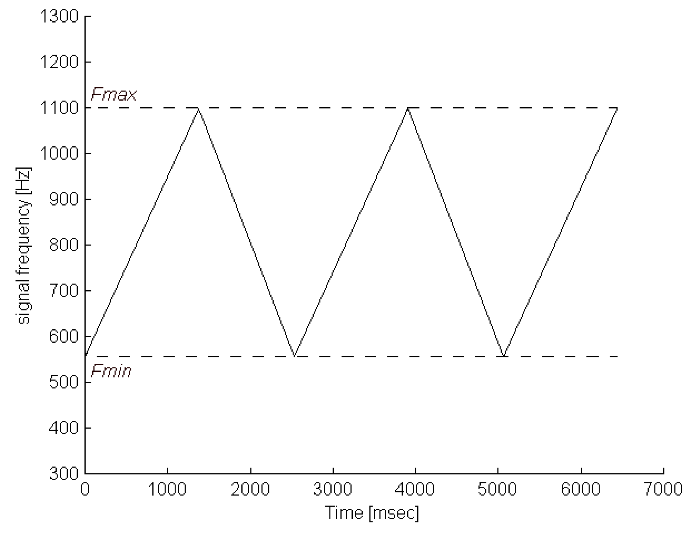
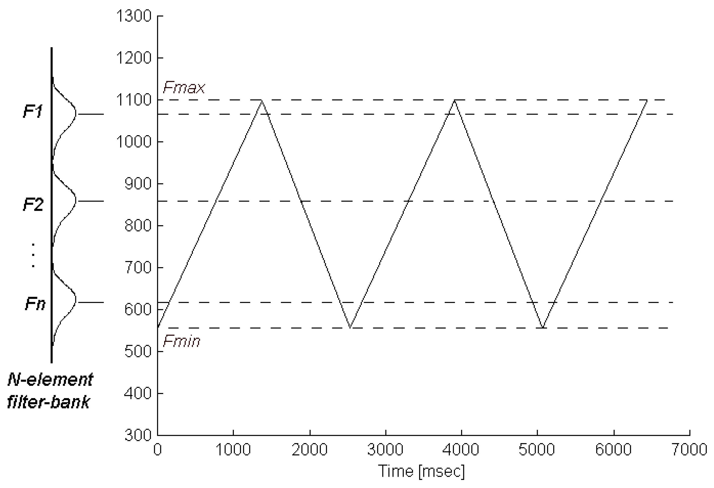
In order to identify a siren signal, it is sufficient to estimate a few points that represent roughly the frequency characteristic curve. This can be obtained using a digital filter-bank of narrow band-pass filters whose center frequencies are distributed in the spectral range from F_min to F_max , as shown in figure 2.

Figure 2. A filter-bank placed inside the dominant frequency range of a siren.

Figure 2. A filter-bank placed inside the dominant frequency range of a siren.

Figure 3. A frequency characteristic curve derived from a recorded signal of an ambulance siren.

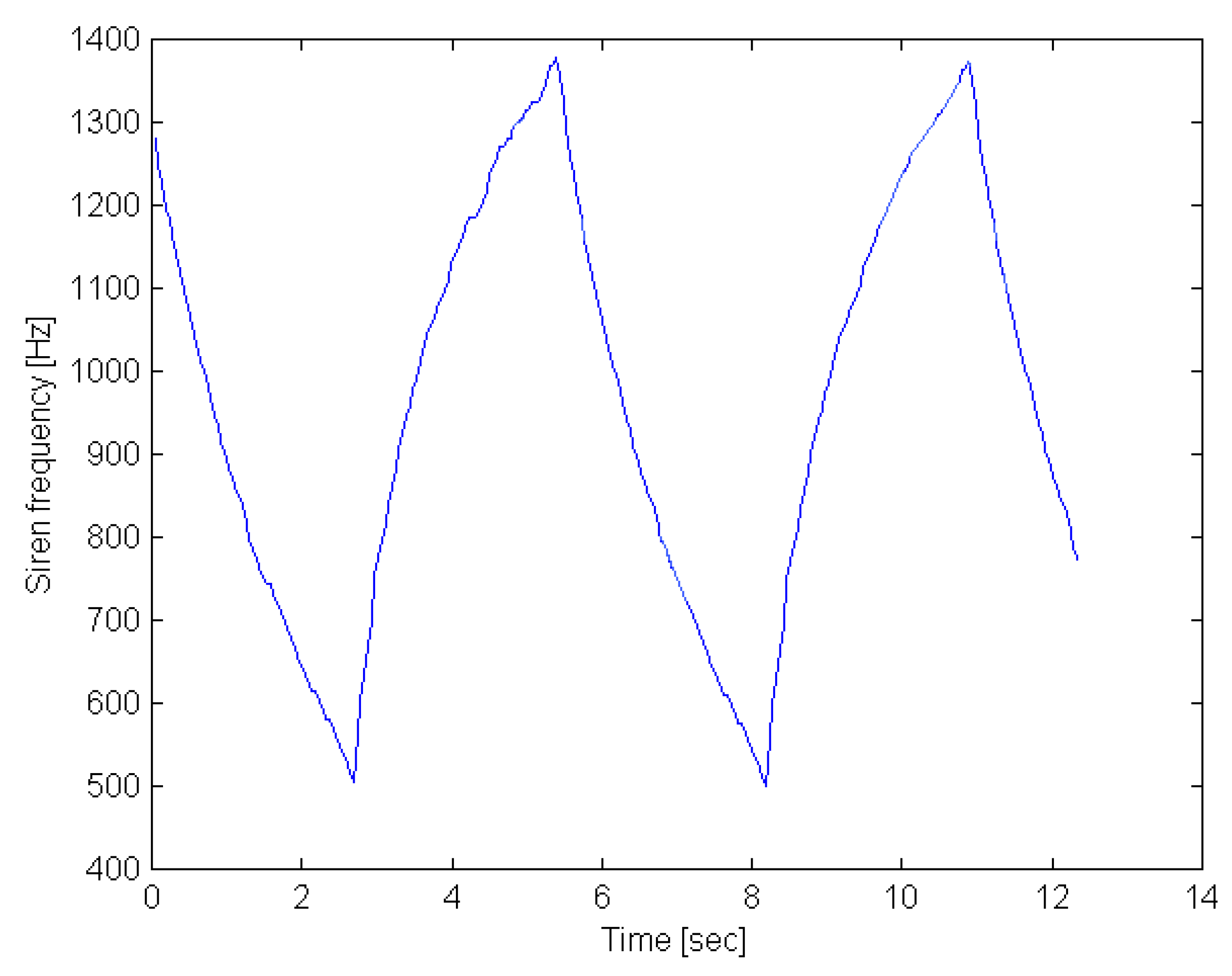
Figure 3. A frequency characteristic curve derived from a recorded signal of an ambulance siren.

According to figure 2, as the instantaneous fundamental frequency of the siren signal changes, it passes successively from the frequency zones that correspond to the pass bands of the filters. Thus, it activates the bank filters, one at the time. A filter is considered as activated when its output signal exceeds a specific threshold. This threshold is adjusted so as to reject sounds below a desired intensity level. By counting the duration between the activation of neighboring filters of the bank, the siren signal can be identified.

Application of the Proposed Approach

The efficiency of the detection method, described in the previous section, was tested for the case of a typical ambulance siren. More specifically, a 10 sec duration signal of the siren was recorded and sampled at 22050 kHz. Subsequently, it was divided into a series of successive snapshots, which correspond to small duration overlapping parts of the signal. Next the spectral content of each snapshot was calculated using the Discrete Fourier Transform, and the dominant frequency component was estimated. In this way, the frequency characteristic curve shown in figure 3 was constructed.

Figure 4. Frequency response of the three-element filter bank.

Figure 4. Frequency response of the three-element filter bank.

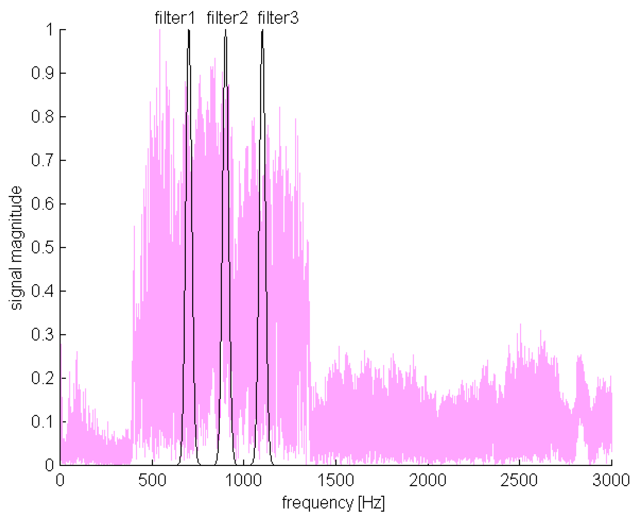
The choice of the necessary number of filters depends on the complexity of this curve. For the current case, 3 filters were employed with center frequencies at 700Hz, 900Hz and 1100Hz, and with 60Hz bandwidth. The frequency response of the three filters is presented in figure 4, with overlapping the magnitude of the siren signal spectrum. The output of each filter, as a function of time, is shown in figure 5. The activation time points due to the siren signal correspond to the time position of the high amplitude peaks. Combination of the three filters output signals provides an estimation of the siren frequency characteristic curve.

Figure 5. Activation of the three filters for a pure siren signal.

Figure 5. Activation of the three filters for a pure siren signal.

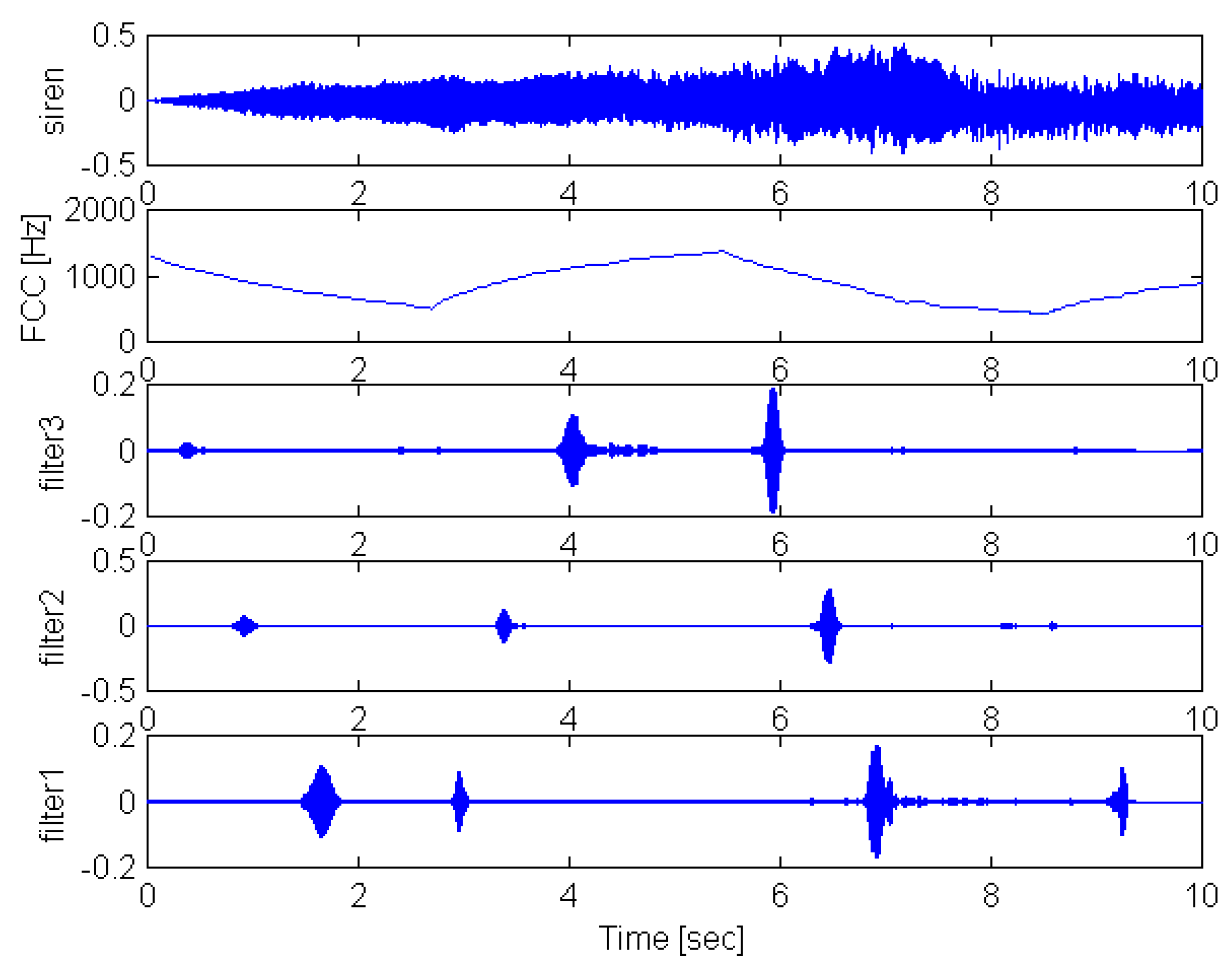
Figure 6. Activation of the three filters for a siren signal in the presence of traffic noise.

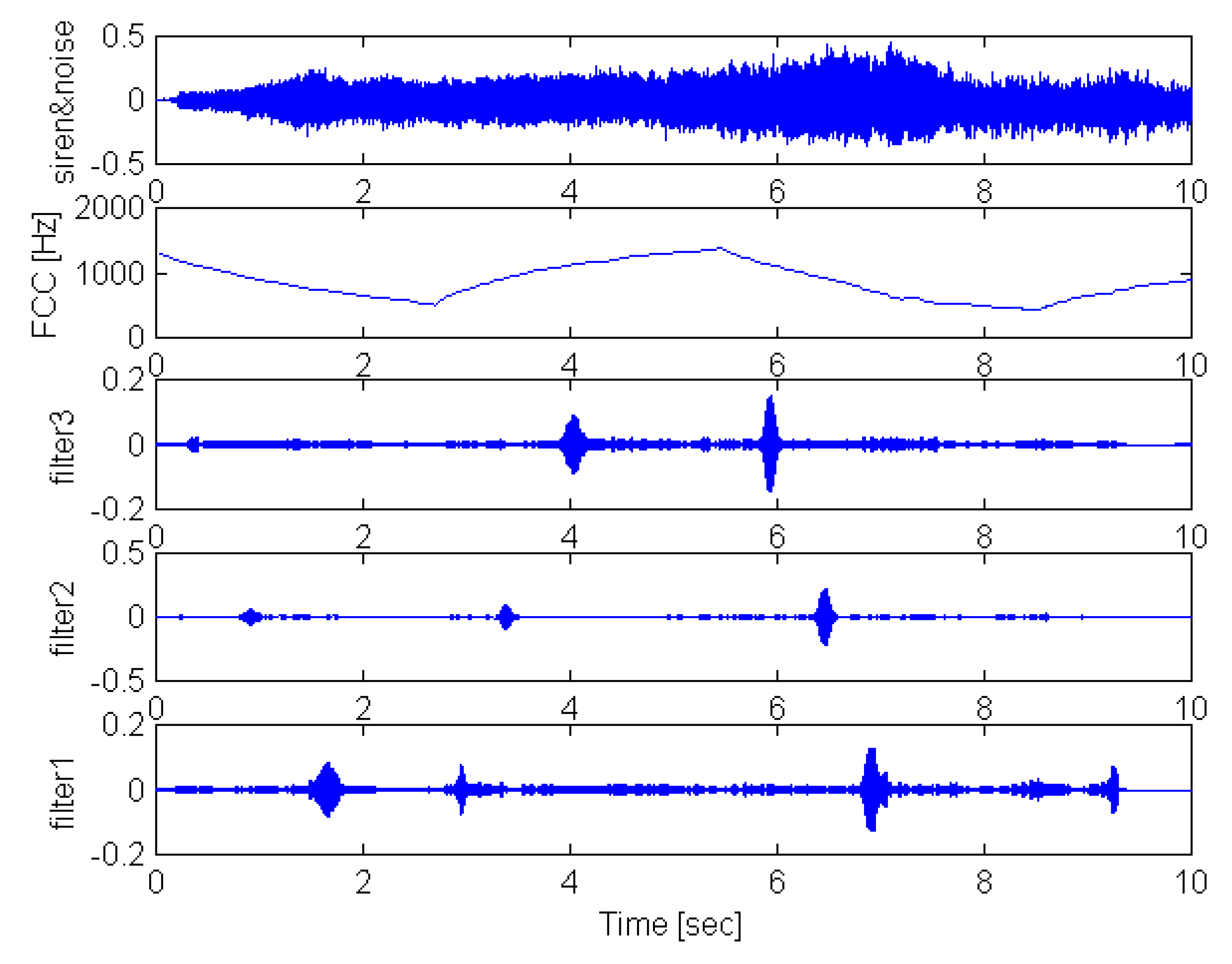
Figure 6. Activation of the three filters for a siren signal in the presence of traffic noise.

The same test was performed for a complex signal consisted of the pure siren signal and a same duration signal corresponding to traffic noise. The two signals were normalized separately so as to equalize their power and subsequently were added together to form a complex signal with a signal to noise ratio of 1:1. From the application of the detection procedure, the results shown in figure 6 were obtained. The clear amplitude peaks provide the activation time points of the filters. The filters were able to isolate the siren signal efficiently even though the presence of the noise was intense. This was achieved because most of the siren energy is concentrated in a quite narrow spectral band. Therefore, inside the narrow bandwidth of each filter, the signal to noise ratio is high enough to avoid the masking of the signal by the noise [5,6,7].

An Implementation of the Filter-Bank using Mechanical Resonators

The siren detection procedure described above can be applied using a microphone and a Digital Signal Processor (DSP) that performs acoustic signature recognition. However, a very simple and efficient approach is presented next, employing a set of mechanical resonant filters to implement a filter-bank, and a simple logic circuit to count the time between successive activation of neighboring filters. Moreover, a scaling down procedure is proposed so that a microsystem may be developed. The proposed approach allows the incorporation of all the necessary elements into a micro electromechanical system, reducing thus the cost, in comparison to a system with conventional microphones and DSPs.

Structure of the mechanical resonant elements

Each mechanical element that is used as a resonant sound sensor [8,9] consists of two parallel cantilever beams with a small plate attached to their free ends, as shown in figure 7.

Figure 7. Mechanical structure of a single resonant element.

Figure 7. Mechanical structure of a single resonant element.

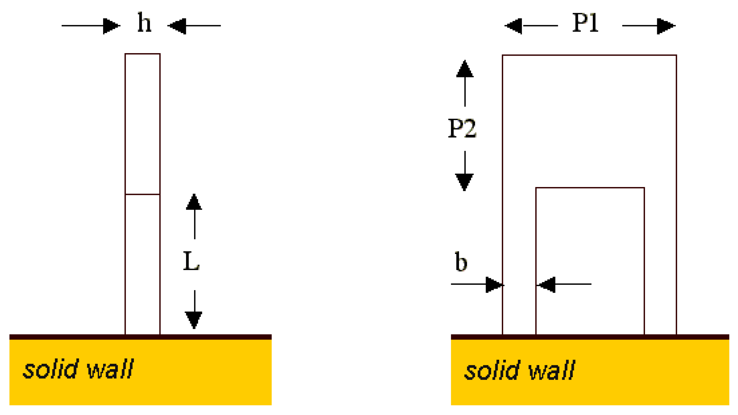
This structure allows the element to collect more energy from the sound field and also to operate as a band pass filter. The two cantilever beams holding the plate, offer an increased stability to the whole structure. The resonant frequency of the element depends on the mechanical properties of its material, dimensions and geometry. If each of the beams is considered as a spring then the total structure can be approximated by the simple equivalent system [10,11]. In this view, the plate is considered as a concentrated mass attached at the ends of two parallel springs whose equivalent spring constants are given by the following equations:

$$I=\frac{(b·h^3)}{12}$$

(1)

$$S_{equiv}=(3·E·I)/L^3$$

(2)

where L is the length, b is the width, h the thickness, E the Young's modulus of elasticity and I the moment of inertia of each beam. By choosing proper values of the above parameters, the elasticity of the beams can easily be adjusted. The resonance frequency of the element can be calculated by:

$$\omega =\sqrt{S_{equiv}/m_{pick-up}}$$

(3)

where m_pick-up is the mass of the plate.

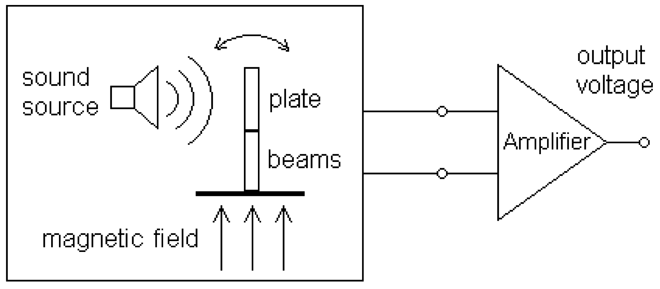
In order to measure the response of the mechanical element, the motion of its plate is monitored employing an electrodynamic transducer as illustrated in figure 8. The mechanical system is located between the poles of a magnet with a properly chosen orientation. The plate is acting as a conductor of length $\mathcal{l}$ that moves inside the magnetic field due to the force of the sound field. This motion induces a voltage across the terminals of the element that is measured with the aid of an instrumentation amplifier.

Figure 8. Electrodynamic transducer.

Figure 8. Electrodynamic transducer.

Electrodynamic transducers

An electrodynamic transducer can be characterized as a reversible sensor since it operates both as a sensor and as a vibration generator [12,13]. In a transducer of this type, a conductor of length $\mathcal{l}$ is positioned in a magnetic field of strength B , and the sound causes the conductor to move across the magnetic lines. The conductor may be a ribbon that is mounted between the poles of a magnet and serves as a pressure-actuated membrane. If the conductor carries an electric current i there results a transducer force F_t that obeys:

$$F_t=B·i·\mathcal{l}$$

(4)

In the current analysis, all the variables are expressed in terms of phasors. We may select the algebraic signs so that to a positive i the corresponding transducer force opposes the exciting force F produced by the sound field. The difference between these two forces is equal to the product of the mechanical impedance Z_m and the velocity υ of the conductor:

$$F-F_t=Z_m·\upsilon$$

(5)

Substitution of equation (4) into (5) results to:

$$F=Z·\upsilon +B·i·\mathcal{l}$$

(6)

where F is the independent variable and i one of the dependent variables. Additionally a transducer voltage V_t appears across the wire due to its motion inside the magnetic field, given by:

$$V_t=B·\mathcal{l}·\upsilon$$

(7)

Finally, the voltage at the terminals of the transducer is given by:

$$V-V_t=Z_e·i=(R+j\omega L)·i$$

(8)

where Z_e is the electrical impedance of the conductor, which is equal to the sum of the resistance R and the reactance jωL of the conductor or the coil.

Equations (6) and (8) may be presented as a matrix form representing an electromechanical two-port system:

$$\left(\begin{array}{c}F\\ V\end{array}\right)=\left(\begin{array}{cc}{Z}_m& B\mathcal{l}\\ -B\mathcal{l}& Z_e\end{array}\right)·\left(\begin{array}{c}\upsilon \\ i\end{array}\right)$$

(9)

For excitors, we consider an arbitrary independent excitation voltage V_o and a load impedance that corresponds to the internal impedance Z_e,o of the voltage source, for which:

$$V_o-V=Z_{e,o}·i$$

(10)

For sensors, one must also account for a similar loading on the mechanical side. The force, F_o, that is to be measured, acts on the transducer through this impedance. For a moving membrane, F_o is related to the force F acting on the membrane by:

$$F_o-F=Z_{m,o}·\upsilon$$

(11)

where Z_m,o is the sound radiation impedance. This impedance is generally small enough so that the Z_m,o = 0 .

Incorporation of the loads and the primary variables F_o and V_o leads to:

$$\left(\begin{array}{c}{F}_o\\ V_o\end{array}\right)=\left(\begin{array}{cc}{Z}_{m,o}+Z_m& B\mathcal{l}\\ -B\mathcal{l}& Z_{e,o}+Z_e\end{array}\right)·\left(\begin{array}{c}\upsilon \\ i\end{array}\right)$$

(12)

which may be rewritten in the following form:

$$\left(\begin{array}{c}\upsilon \\ i\end{array}\right)=\frac{1}{(Z_m+Z_{m,o})·(Z_e+Z_{e,o})+{(B\mathcal{l})}^2}·\left(\begin{array}{cc}{Z}_e+Z_{e,o}& -B\mathcal{l}\\ B\mathcal{l}& Z_m+Z_{m,o}\end{array}\right)·\left(\begin{array}{c}{F}_o\\ V_o\end{array}\right)$$

(13)

The terms of the main diagonal of the matrix above represent the mechanical and the electrical admittance of the sensor (for V_o = 0 ) and the excitor (for F_o = 0 ). The mechanical input impedance of the sensor is given by:

$$\begin{array}{c}{\frac{F_o}{\upsilon }|}_{V_o=0}=Z_{m,o}+Z_m+\frac{{\left(B\mathcal{l}\right)}^2}{(Z_e+Z_{e,o})}\\ =r+\frac{s}{j\omega }+j\omega m+\frac{{\left(B\mathcal{l}\right)}^2}{R+R_o+j\omega L}\end{array}$$

(14)

The additional damping represented by the fourth term, increases as the electrical impedances decrease and it is greatest if the output terminals are short-circuited. The transfer function of the sensor is represented from the lower left term of the matrix of equation (13):

$${\frac{F_o}{\upsilon }|}_{V_o=0}=\frac{-B\mathcal{l}}{(Z_m+Z_{m,o})·(Z_e+Z_{e,o})+{\left(B\mathcal{l}\right)}^2}$$

(15)

The Proposed Siren Detection System

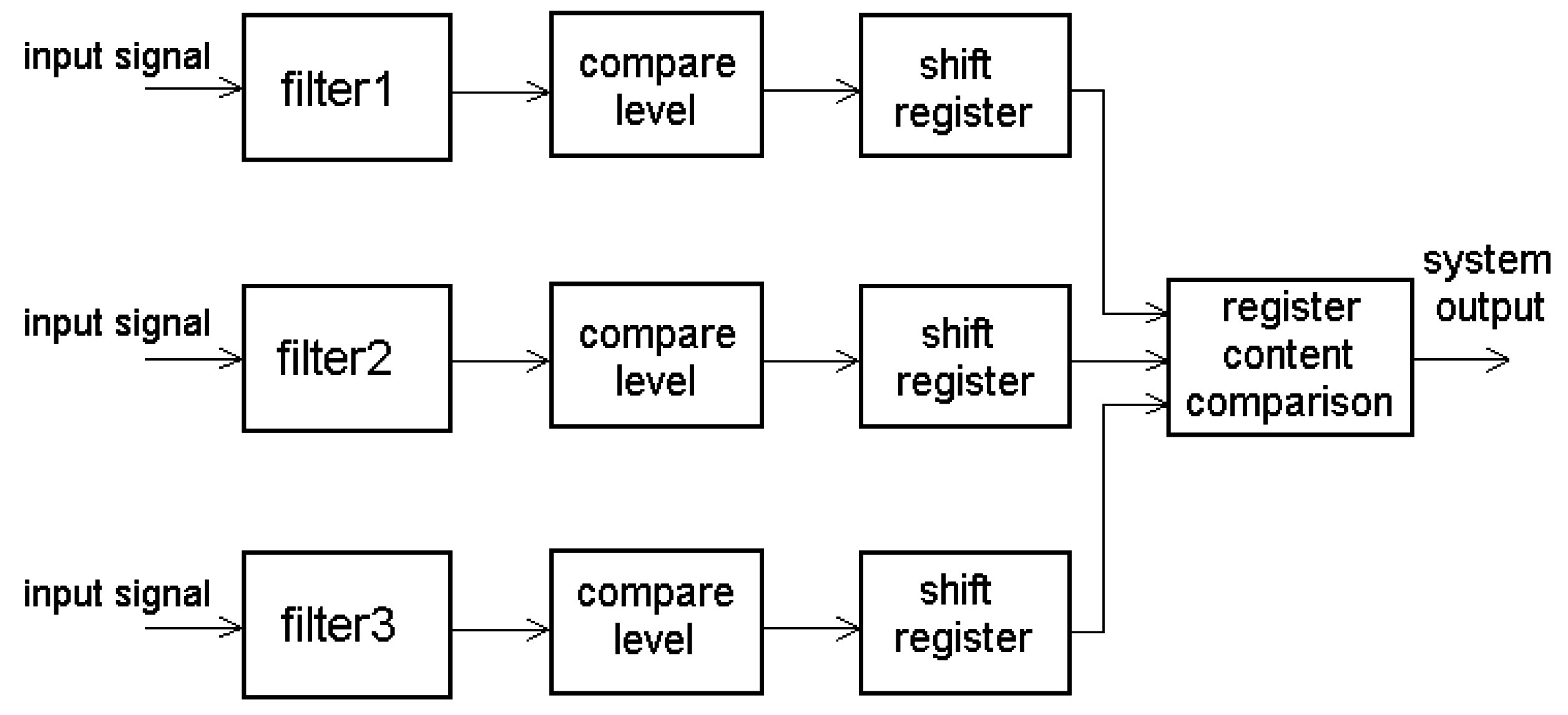
An implementation of the proposed siren detector system is illustrated in the block diagram of figure 9. The output amplitude of each filter is continuously measured and it is converted to a dc voltage. Then the derived voltage is compared with a threshold level and thus a binary output value is obtained. This binary value, which represents the activation state of each filter, must be stored for a half period time distance. For this purpose, three shift registers, one for each filter, are employed.

The length of the registers must be as short as possible, while it must be sufficient to store the activation state of the filters for a time period approximately equal to half of the period of the characteristic curve. The pulse rate of the register clock must be selected so as to ensure that the registers are able to follow the changes of the activation state of the filters

Figure 9. Block diagram of the siren detection system.

Figure 9. Block diagram of the siren detection system.

The frequency characteristic curve depicted in figure 3 has an exponential form. However, parts of the curve can be approximated with straight lines. Considering the descending part of the curve from 1100Hz to 700Hz and using a linear approximation, the relation between signal frequency and time can be expressed as:

frequency = α · time, α ≈ 0.3 Hz/m sec

Since a filter remains active as long as the signal fundamental frequency remains inside the pass-band of the filter, then the activation time of the filter, using the linear approximation in the band [700Hz, 1100Hz], is analogous to its bandwidth:

$$timeofactivation\approx \frac{filterbandwidth}{\alpha }$$

Figure 10. The three binary activation patterns corresponding to a successfully detected siren signal.

Figure 10. The three binary activation patterns corresponding to a successfully detected siren signal.

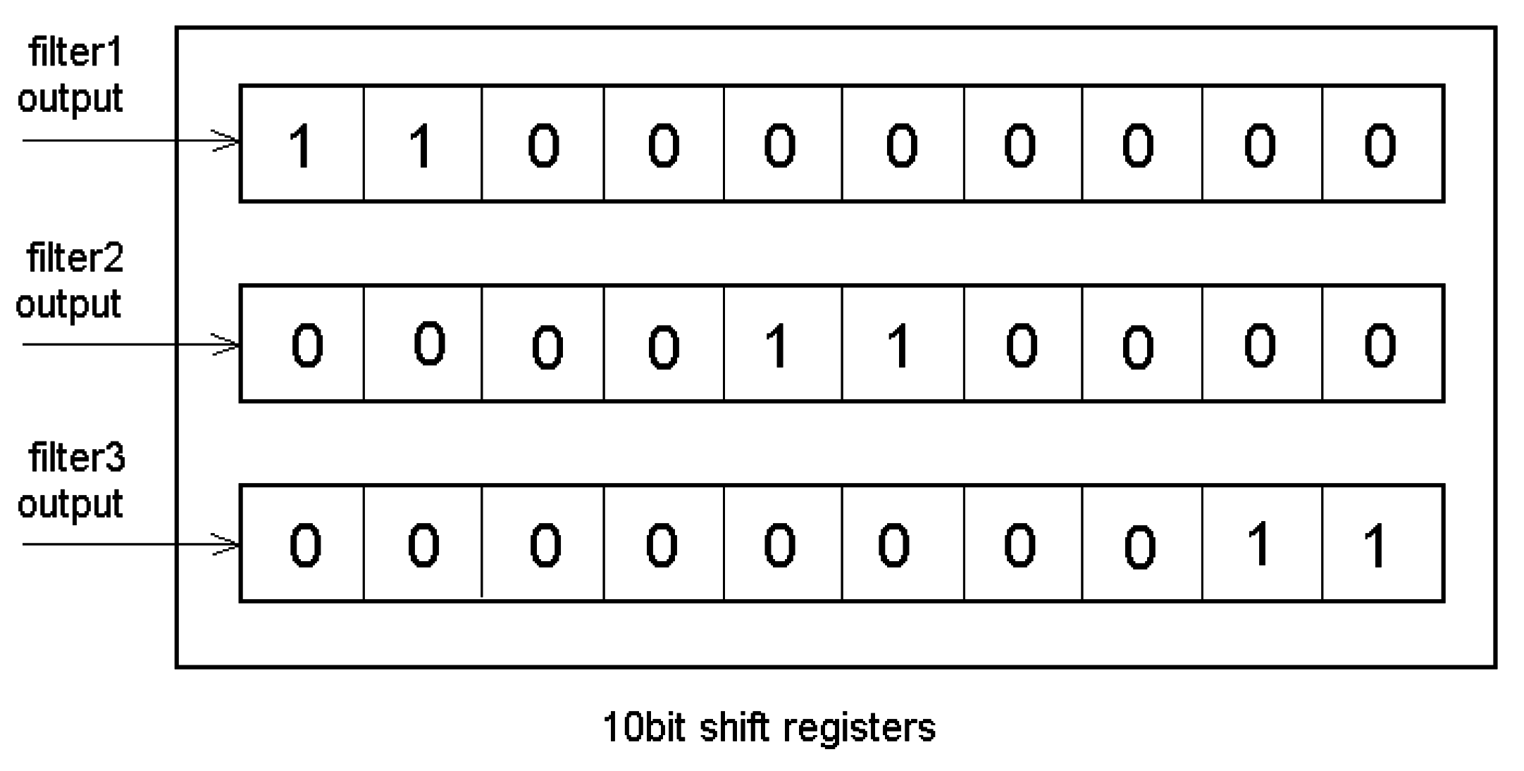
If the center frequencies of the filters are set to 700Hz, 900Hz and 1100 Hz, and the pulse rate of the clock is determined to 7 pulses/sec, then the recording of each filter output for a time distance: $\frac{1130-670}{0.3}\approx 1.5\text{sec}$ can be achieved using shift registers of 10 bits. According to the synchronization between the clock pulses and the siren signal, a filter activation value holds the value of 1 for one or two successive clock pulses. This will cause the appearance of the value of 1 at one or two adjacent positions in the corresponding register.

Signal detection is performed by comparing the values stored in the three registers to the three activation patterns that are illustrated in figure 10. An important condition for the successful recognition is that the sound intensity of the siren signal is high enough to activate the filters, while the intensity of the ambient noise is relatively lower within the pass-bands of the filters. For this reason the sensitivity of the electrodynamic filters has to be adjusted properly.

Experimental Results on the Resonant Curves of the Mechanical Filters

Several elements of various dimensions were tested as mechanical resonators; dimensions are presented in Table 1 and their corresponding resonance curves are shown in Figure 11 and Figure 12. The vertical axis of the plots represents the normalized output voltage of the amplifier.

Table 1. Dimensions of the tested elements.

Element	Beam Length L[cm]	Beam width b[cm]	Element thickness h[µm]	Plate width P1 [cm]	Plate height P2[cm]	Frequency of resonance [Hz]
1	0.35	0.20	20	1.18	0.31	207
2	0.31	0.28	20	1.28	0.60	215
3	0.43	0.16	60	1.38	0.16	320
4	0.35	0.20	20	1.18	0.20	340
5	0.35	0.20	20	1.18	0.10	477
6	0.08	0.16	20	0.69	0.60	615
7	0.13	0.20	20	1.18	0.10	622
8	0.08	0.20	20	1.18	0.10	1190

Table 1. Dimensions of the tested elements.

Element	Beam Length L[cm]	Beam width b[cm]	Element thickness h[µm]	Plate width P1 [cm]	Plate height P2[cm]	Frequency of resonance [Hz]
1	0.35	0.20	20	1.18	0.31	207
2	0.31	0.28	20	1.28	0.60	215
3	0.43	0.16	60	1.38	0.16	320
4	0.35	0.20	20	1.18	0.20	340
5	0.35	0.20	20	1.18	0.10	477
6	0.08	0.16	20	0.69	0.60	615
7	0.13	0.20	20	1.18	0.10	622
8	0.08	0.20	20	1.18	0.10	1190

Figure 11. Resonance curves of No1, No2, No3 and No4 tested elements.

Figure 11. Resonance curves of No1, No2, No3 and No4 tested elements.

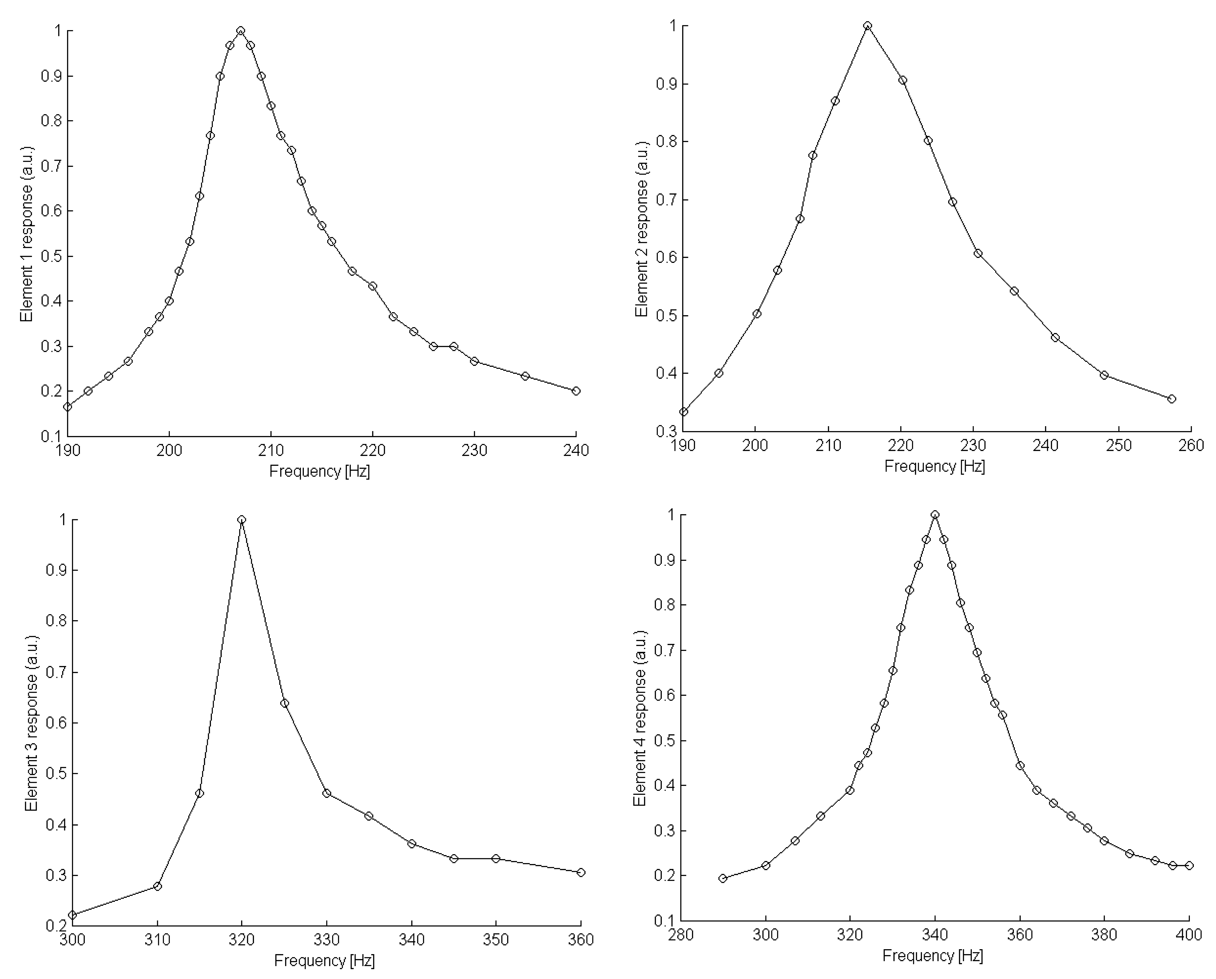
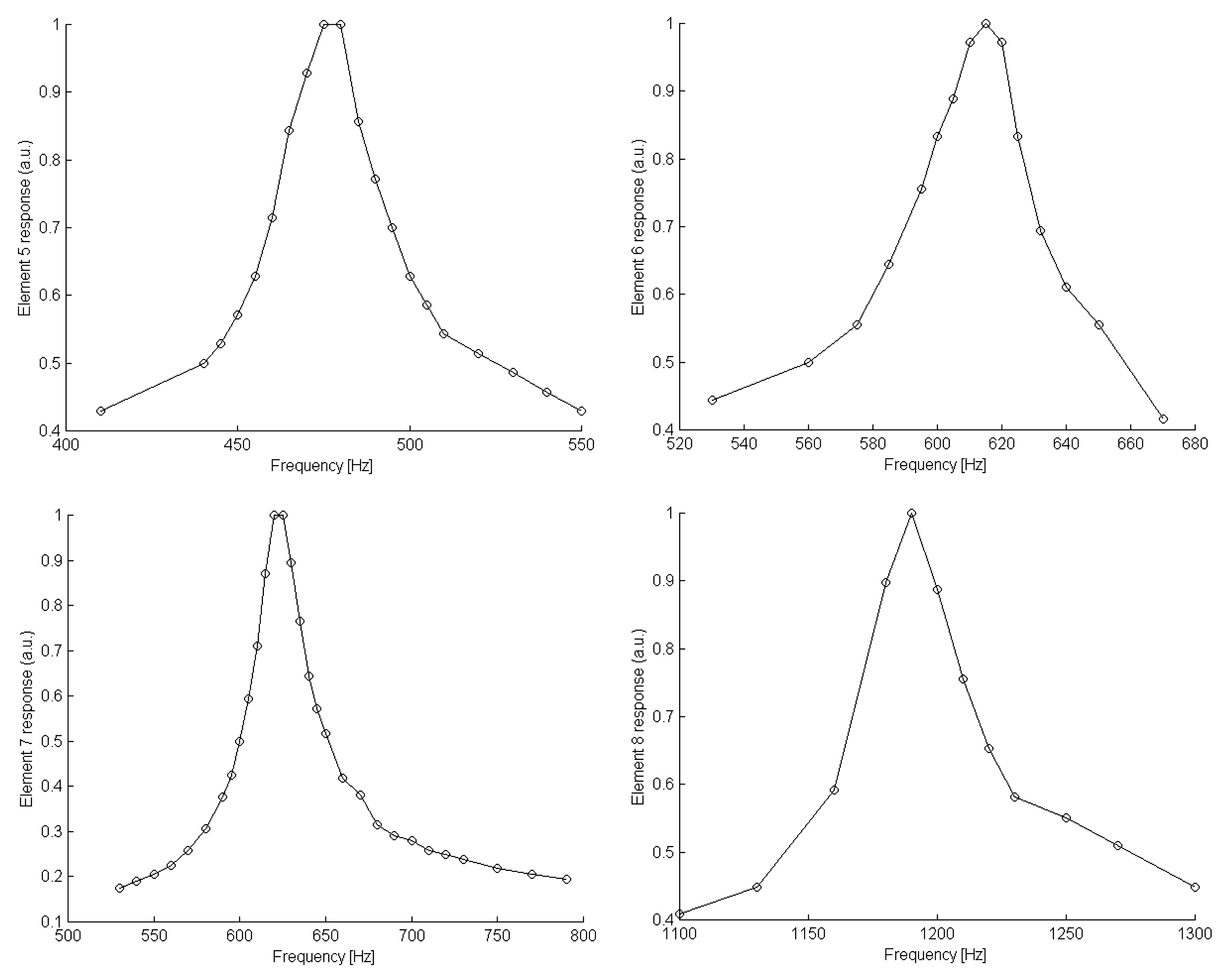
It is worth noting that, close to resonance, the mechanical impedance of the element is essentially affected by the damping constant r . Since the mechanical impedance determines the width of resonance then it is the value of r that crucially affects the bandwidth of the resonant sensor. By inspection of the two aforementioned figures it becomes apparent that elements with larger plates exhibit a wider bandwidth. This was expected since a large plate is subjected to a higher damping in comparison to a smaller one.

Figure 12. Resonance curves of No5, No6, No7 and No8 tested elements.

Figure 12. Resonance curves of No5, No6, No7 and No8 tested elements.

The sensitivity of the constructed resonant sensors was measured using as a reference a uni- directional YAMAHA DM-100 dynamic microphone. The sensitivity of the microphone is 1V/µBar. The measurements were performed by adjusting the sound source frequency to the resonance frequency of the testing element and then measuring the output voltage of the system. The sound pressure was also measured with the microphone in the vicinity of the mechanical element. The sensor sensitivity was calculated dividing the output voltage of the sensor by the measured sound pressure value. This procedure was repeated for several values of sound pressure and the curve shown in figure 13 was obtained, which shows that the tested element exhibits an almost linear behavior within the measured pressure range.

Figure 13. Sound pressure sensitivity of a tested mechanical element.

Figure 13. Sound pressure sensitivity of a tested mechanical element.

Figure 14. Experimentally obtained polar diagram of a 150 Hz resonant element.

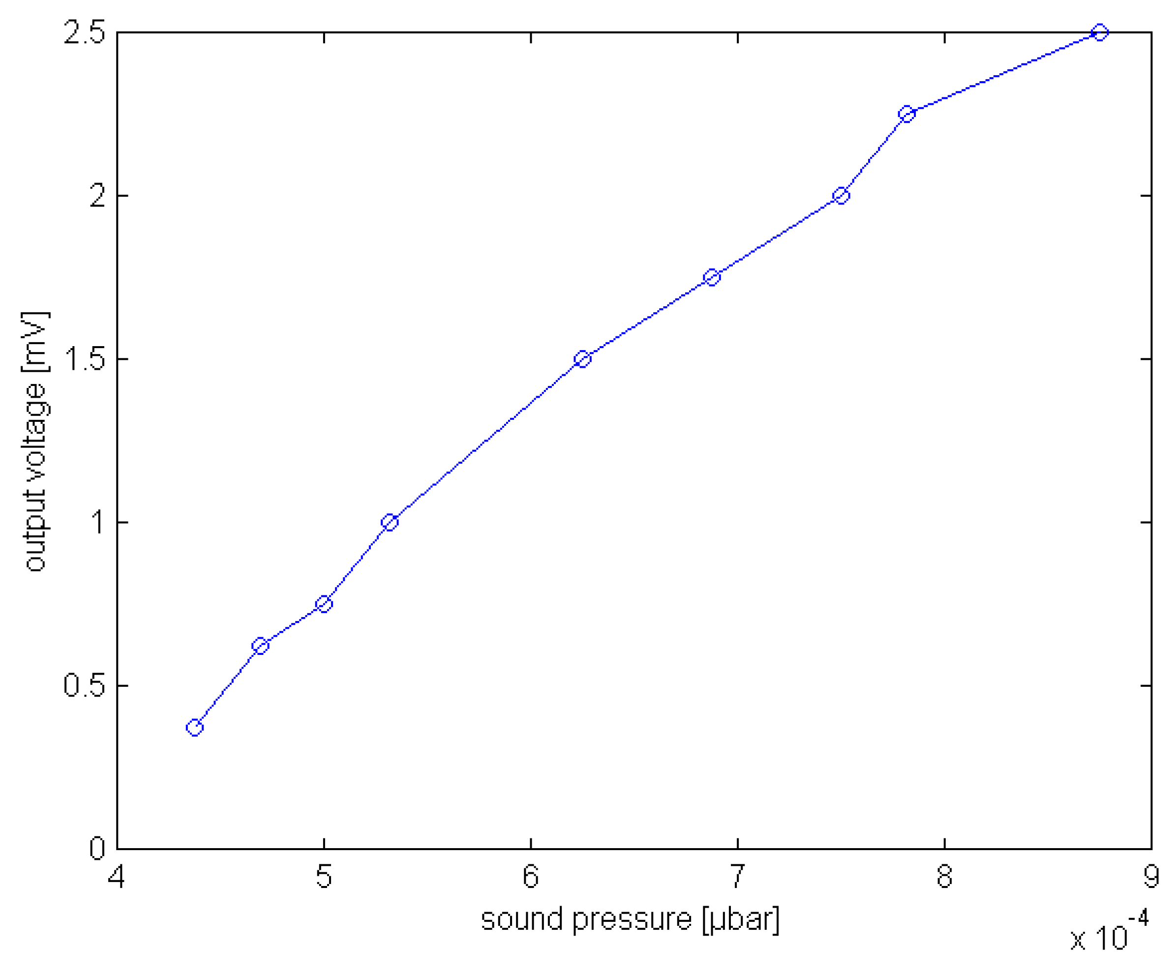
Figure 14. Experimentally obtained polar diagram of a 150 Hz resonant element.

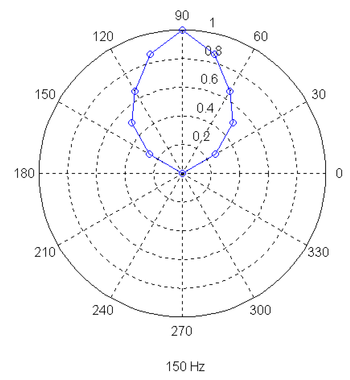
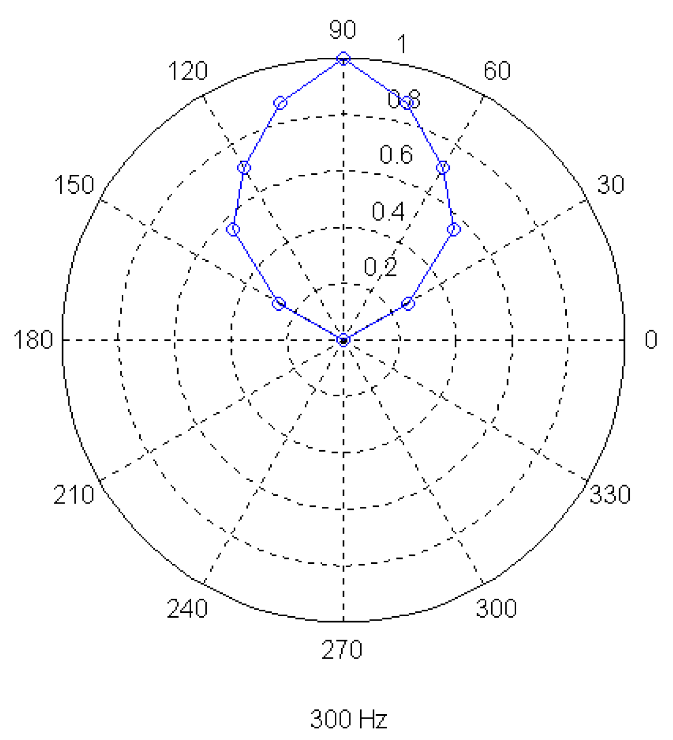
Moreover, a series of measurements was performed in order to obtain the directional properties of the mechanical filters under consideration. Three elements were used for this purpose, with resonance frequencies at 150 Hz, 300 Hz and 500 Hz. All dimensions of the tested elements were similar except for the length of the beams, which was properly chosen so as to obtain the aforementioned resonance frequencies. Each element was positioned with a predefined orientation and the sound source frequency was adjusted to the resonance frequency of the element. The output of the filter was measured for several directions of the incident sound by moving the source on a circle around the element position. The obtained polar diagrams, which are presented in figure 14, figure 15 and figure 16, indicate that the tested elements exhibit the higher sensitivity for sounds coming from the frontal direction, while they become almost insensitive for directions over 150 degrees and under 30 degrees. Therefore the tested mechanical elements may be used as directional sound sensors.

Figure 15. Experimentally obtained polar diagram of a 300 Hz resonant element.

Figure 15. Experimentally obtained polar diagram of a 300 Hz resonant element.

Figure 16. Experimentally obtained polar diagram of a 500 Hz resonant element.

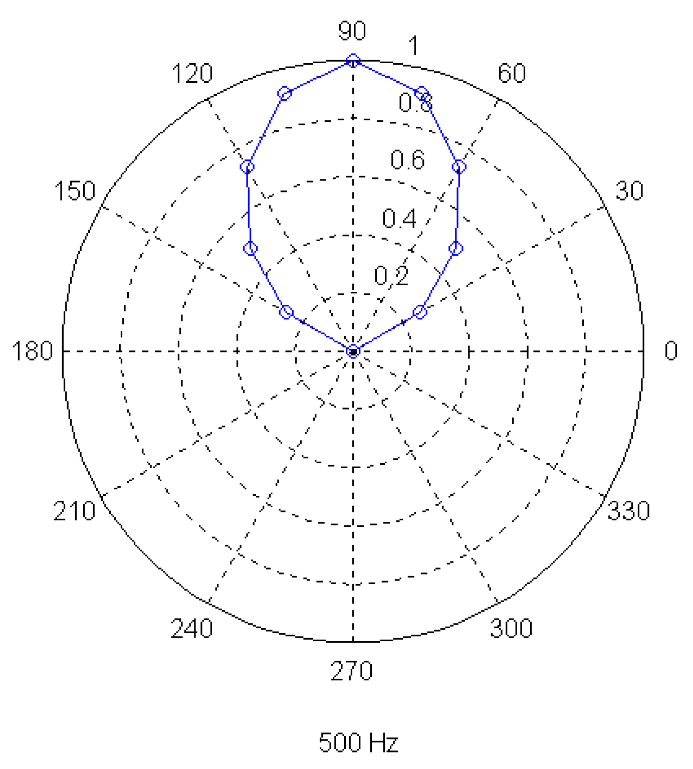
Figure 16. Experimentally obtained polar diagram of a 500 Hz resonant element.

Toward the Implementation of a Microsystem

A scale down procedure can be applied to the proposed structure in order to implement a microsystem [14,15,16,17,18,19]. The simple geometry of the structure allows the combination of a set of electromechanical filters for the implementation of a low cost, passive, narrow filter bank. It is noticed that siren recognition is one civilian application whereas there is a vast number of defense applications requiring low power, small size, etc. microsystems.

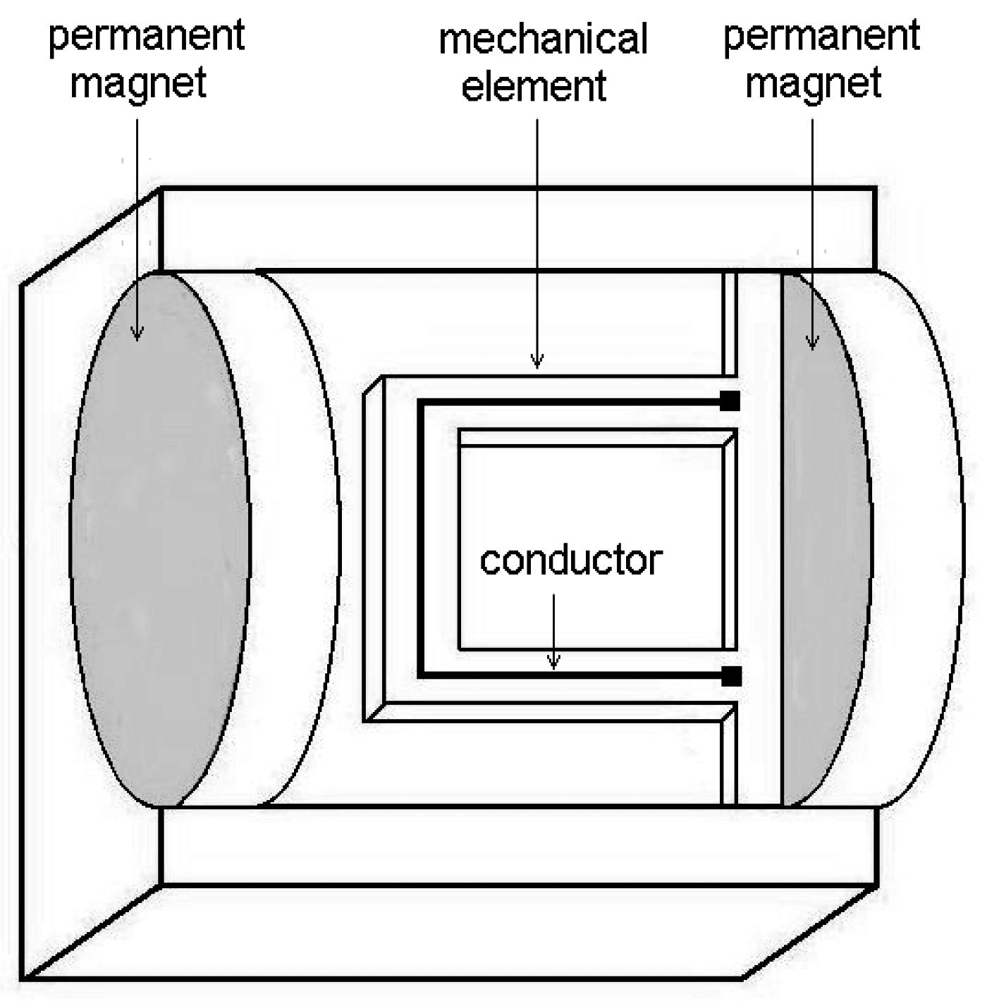
A possible geometry of a microsystem is shown in figure 17. The resonant system is placed in a strong magnetic field generated by a pair of miniature permanent magnets, which may be electroplated. The resulting motion of the resonator is detected by measuring the induced voltage on the moving conductor that is attached to the mechanical element. As shown in the figure, the magnetic field runs parallel to the length of the element and thus perpendicular to the direction of the elements motion. The conductor that follows the perimeter of the resonant element moves with it in the magnetic field.

Figure 17. Proposition for a microsystem.

Figure 17. Proposition for a microsystem.

The voltage induced between the two ends of the conductor is given by Equation (7), which can be written in the form:

$$V=B·{\mathcal{l}}_a·2\pi ·f·x_{end}$$

(16)

where ${\mathcal{l}}_a$ is the width of the element and x_end the displacement of the element measure at its free end. Making the assumption that the maximum allowable displacement is proportional to the length of the element, a relative displacement a_rel can be defined such as:

$$a_{rel}=x_{end}/{\mathcal{l}}_a$$

(17)

where ${\mathcal{l}}_b$ is the length of the element.

By choosing some values for the above parameters, the order of the generated voltage can be derived. Thus for: B = 1 tesla , a_rel = 0.01 , ${\mathcal{l}}_a$ = 100μ , ${\mathcal{l}}_b$ = 100μ and f = 500 Hz the induced voltage is:

V = 2π·500·0.01·10^-4·10^-4·1 ≈ 0.3πVolt

It is clear the value of the induced voltage reduces as the dimensions of the mechanical element are shortened and it increases as the magnetic field is strengthened. Therefore, if it is desired to design a smaller system, the magnetic field must be larger. Generally, to obtain a high magnetic field strength close to the saturation value of the magnetic material, the spacing between the two magnets must be small compared to their diameter, and the length of each magnet must be large compared to its diameter.

Conclusion

It has been shown that a macro-system incorporating three mechanical resonant filters can be implemented in order to detect the siren sound of emergency vehicles even in the noisy environment of urban roads. The application of such a system can provide an efficient control of traffic lights. The frequency response, the sensitivity and the directional properties of several mechanical elements, employed as sound sensors, have been demonstrated. Finally, the performance of a prototype has been studied and a scaling-down procedure has been proposed.

References and Notes

- Mitchell, W.L. Traffic light control for emergency vehicles. US 4443783, 1984. [Google Scholar]
- Obeck, C.J. Traffic signal control for emergency vehicles. US 5014052, 1991. [Google Scholar]
- Markson, R.J.; Govaert, J.A. Optical warning system. US 5057820, 1991. [Google Scholar]
- Rose, C.R.; et al. Emergency vehicle detection system. US 5894279, 1999. [Google Scholar]
- Gold, B.; Morgan, N. Speech and audio signal processing; John Wiley: NY, 2000; Chapter 15; p. 210. [Google Scholar]
- Moore, B.C.J. An Introduction to the Psychology of Hearing; Academic Press: London, 1997; Chapter 3; p. 96. [Google Scholar]
- Norton, M.P. Fundamentals of noise and vibration analysis for engineers; Cambridge University Press: UK, 1999; Chapter 4; p. 248. [Google Scholar]
- Fragoulis, D.K.; Avaritsiotis, J.N. Microsystems for acoustical signal detection applications. In Accepted for publication in the Proceedings of the International Conference on MMN, Athens, November 2000.
- Cremer, L.; Heckl, M.; Ungar, E. Structure-borne sound; Springer-Verlag: Berlin, 1988; Chapter 1; p. 32. [Google Scholar]
- Fertis, D.G.; Chidiac, G.E. Dynamically equivalent systems for beams and frames. In Proceedings of the 21st Midwestern Mechanics Conference. Michigan Technological University, Houghton, Michigan, 1989; Vol. 15, pp. 399–401.
- Fertis, D.G. Vibration of beams and frames by using dynamically equivalent systems. In Proceedings of the structural Dynamics and Vibration Symposium. Energy-Sources Technology Conference and Exhibition, ASME, New Orleans, LA, January 1994; pp. 23–26.
- McConnell, K.G. Vibration testing -Theory and practice; John Wiley: NY, 1995; Chapter 4; p. 161. [Google Scholar]
- Doebelin, E.O. Measurement Systems: Application and design; McGraw-Hill: Singapore, 1990; Chapter 6; p. 498. [Google Scholar]
- Garder, J.W. Microsensors: Principles and Applications; John Wiley: NY, 1994; Chapter 7; p. 201. [Google Scholar]
- Howe, R.T. Resonant Microsensors, Technical Digest. In 4th International Conference on Solid- State Sensors and Actuators, Tokyo, Japan, June 1987; pp. 843–848.
- Micromechanical RF filters excited by the Lorentz force. J. Micromech. Microeng. 1999, 9, 78–84.
- Lin, L.; et al. Micromechanical Filters for Signal Processing. Microelectromechanical Systems 1998, 7(3), 286–294. [Google Scholar] [CrossRef]
- Cleland, N.A.; Roukes, M.L. Fabrication of high Frequency nanometer scale mechanical resonators from bulk Si crystals. Appl. Phys. Lett. 1996, 69(18), 2653–2655. [Google Scholar]
- Nguyen, C.T.C. High-Q micromechanical oscillators and filters for communications. In Proc. IEEE Int. Symp. Circuits and Systems, Hong Kong, June 9-12; 1997; pp. 2825–2828. [Google Scholar]
- Sample Availability: Available from the author.
© 2001 by MDPI (http://www.mdpi.net). Reproduction is permitted for noncommercial purposes.
Share and Cite
MDPI and ACS Style
Fragoulis, D.K.; Avaritsiotis, J.N. A Siren Detection System based on Mechanical Resonant Filters. Sensors 2001, 1, 121-137. https://doi.org/10.3390/s10400121
AMA Style
Fragoulis DK, Avaritsiotis JN. A Siren Detection System based on Mechanical Resonant Filters. Sensors. 2001; 1(4):121-137. https://doi.org/10.3390/s10400121
Chicago/Turabian StyleFragoulis, Dimitris K., and John N. Avaritsiotis. 2001. "A Siren Detection System based on Mechanical Resonant Filters" Sensors 1, no. 4: 121-137. https://doi.org/10.3390/s10400121