Collaborative Localization in Wireless Sensor Networks via Pattern Recognition in Radio Irregularity Using Omnidirectional Antennas

Abstract
:
1. Introduction
2. Problem Formulation
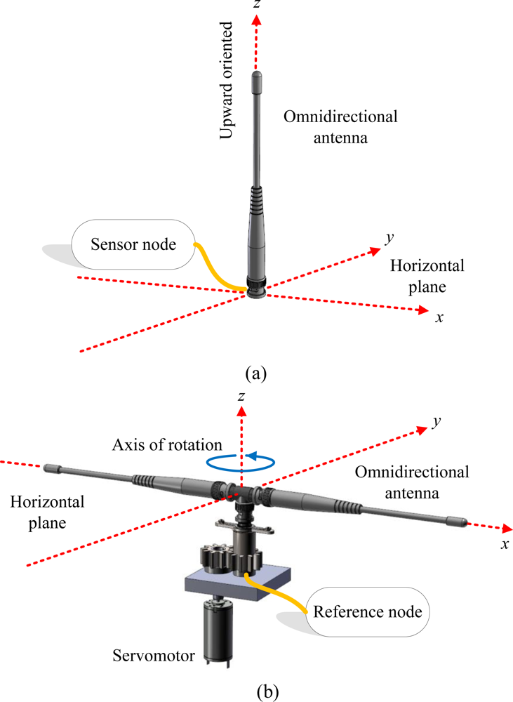
2.1. Network Configuration
- ➢ V is a set of nodes in the network, and V = {S, R}; S is a set of sensor nodes equipped with RSSI sensors, and S = {s1, s2, …, snum_S}; R is a set of reference nodes equipped with servomotor-controlled external antennas, and R = {r1, r2, …, rnum_R}. num_S is the number of sensor nodes; and num_R is the number of reference nodes.
- ➢ Sensor nodes S of the network do not know their location information.
- ➢ Physical positions of R are obtained by manual placement or external means. These nodes are the basis of the localization system.
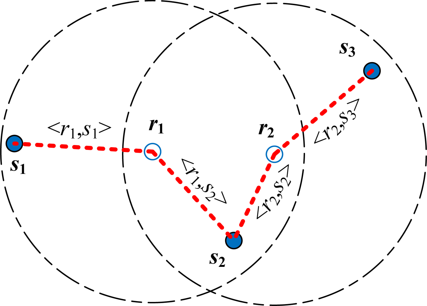
- ➢ <ri, sj> ∈ E. It is sustainable if the distance between ri and sj is lesser than the communication range of ri.
- ➢ Given that a network G = (V, E) and R is with their physical position (xr, yr), for all r ∈ R, the goal of the localization system is to estimate the locations (xs, ys) of as many s ∈ S.
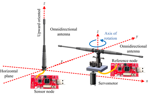
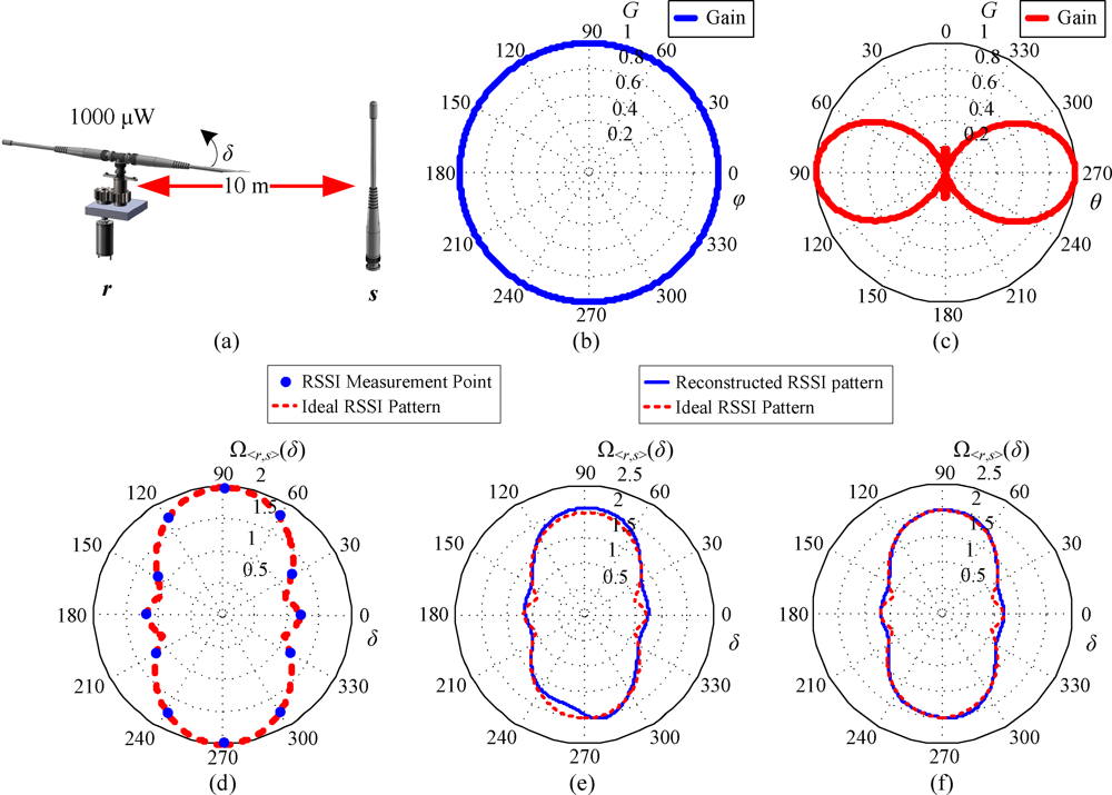
2.2. Configurations of External Antennas
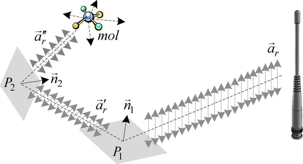
2.3. Theoretical Justification of Antenna Configurations
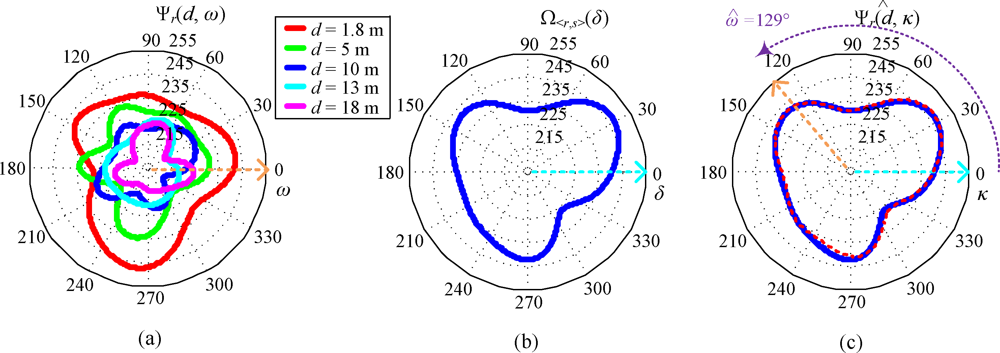
2.4. RSSI Pattern
3. Localization Using Robust Correlation Estimator
4. Collaborative Localization Scheme Using Multiple Reference Nodes
5. Experimental Results
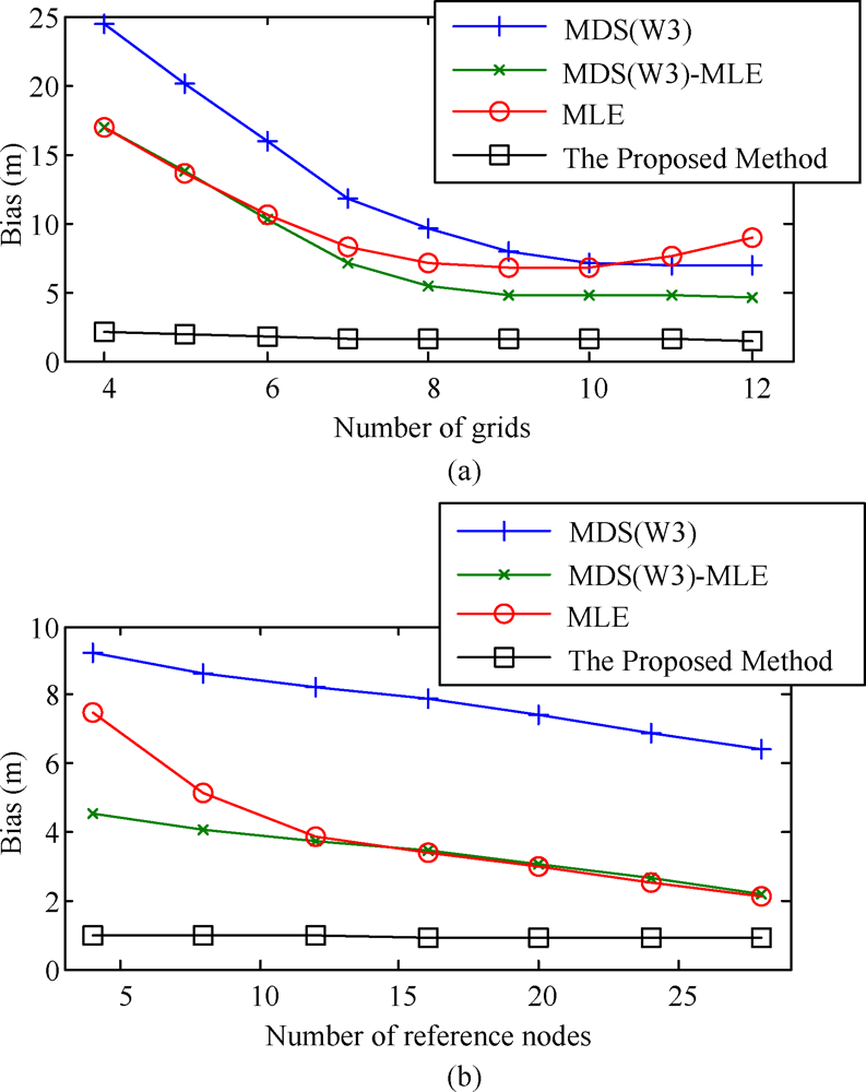
5.1. Performance Evaluations using Computer Simulations
5.2. Performance Evaluations in Real-World Scenarios
6. Conclusions
Acknowledgments
References and Notes
- Chong, C.Y.; Kumar, S.P. Sensor networks: Evolution, opportunities, and challenges. Proc. IEEE 2003, 91, 1247–1256. [Google Scholar]
- Culler, D.; Estrin, D.; Srivastava, M. Overview of sensor networks. Computer 2004, 37, 41–49. [Google Scholar]
- Martinez, K; Hart, J.K.; Ong, R. Environmental sensor networks Computer 2004, 37, 50–56.
- Jiang, J.A.; Chen, C.P.; Chuang, C.L.; Lin, T.S.; Tseng, C.L.; Yang, E.C.; Wang, Y.C. CoCMA: Energy-Efficient Coverage Control in Cluster-based Wireless Sensor Networks using a Memetic Algorithm. Sensors 2009, 9, 4918–4940. [Google Scholar]
- Li, J.; Andrew, L.L.; Foh, C.H.; Zukerman, M.; Chen, H.-H. Connectivity, Coverage and Placement in Wireless Sensor Networks. Sensors 2009, 9, 7664–7693. [Google Scholar]
- Estrin, D.; Culler, D.; Pister, K.; Sukhatme, G. Connecting the physical world with pervasive networks. IEEE Pervasive Comput 2002, 1, 59–69. [Google Scholar]
- Savarese, C.; Rabaey, J.M.; Reutel, J. Localization in distributed Ad hoc wireless sensor networks. Proceedings of the ICASSP, Salt Lake City, UT, USA, May 2001; pp. 2037–2040.
- Rabaey, J.M.; Ammer, M.J.; da Silva, J.L., Jr.; Patel, D.; Roundy, S. PicoRadio supports ad hoc ultra-low power wireless networking. Computer 2002, 33, 42–48. [Google Scholar]
- Basagni, S.; Chlamtac, I.; Syrotiuk, V.; Woodward, B. A distance routing effect algorithm for mobility (DREAM). Proceedings of the MOBICOM, Dallas, TX, USA, October 1998; pp. 76–84.
- Hu, Y.; Perrig, A.; Johnson, D. Packet leashes: A defense against wormhole attacks in wireless ad hoc networks. Proceedings of the INFOCOM, San Francisco, CA, USA, March 2003; pp. 1976–1986.
- Lazos, L.; Poovendran, R. Energy-aware secure multicast communication in ad hoc networks using geographic location information. Proceedings of the ICASSP, Hong Kong, China, April 2003; 6, pp. 201–204.
- Al-Karaki, J.N.; Kamal, A.E. Routing techniques in wireless sensor networks: A survey. IEEE Trans. Wireless Commun 2004, 11, 6–28. [Google Scholar]
- Savvides, A.; Han, C.; Srivastava, M. Dynamic fine-grained localization in ad hoc networks of sensors. Proceedings of the 7th Annual International Conference on Mobile Computing and Networking, Rome, Italy, July 16–21, 2001; pp. 166–179.
- Djuknic, G.M.; Richton, R.E. Geolocation and Assisted GPS. Computer 2001, 34, 123–125. [Google Scholar]
- Sheu, J.P.; Chen, P.C.; Hsu, C.S. A Distributed Localization Scheme for Wireless Sensor Networks with Improved Grid-Scan and Vector-Based Refinement. IEEE Mobile Comput 2008, 7, 1110–1123. [Google Scholar]
- Gutiérrez, Á.; González, C.; Jiménez-Leube, J.; Zazo, S.; Dopico, N.; Raos, I. A Heterogeneous Wireless Identification Network for the Localization of Animals Based on Stochastic Movements. Sensors 2009, 9, 3942–3957. [Google Scholar]
- Pottie, G.J.; Kaiser, W.J. Wireless Integrated Network Sensors. Comm. ACM 2000, 43, 51–58. [Google Scholar]
- Priyantha, N.B.; Chakraborty, A.; Balakrishnan, H. The Cricket Location-Support System. Proceedings of the MobiCom, Boston, Massachusetts, USA, August 2000; pp. 32–43.
- Savvides, A.; Han, C.C.; Strivastava, M.B. Dynamic Fine-Grained Localization in Ad hoc Networks of Sensors. Proceedings of the MobiCom, Rome, Italy, July 2001; pp. 166–179.
- Pahlavan, K.; Li, X.; Makela, J. Indoor geolocation science and technology. IEEE Commun. Mag 2002, 40, 112–118. [Google Scholar]
- Li, X.; Pahlavan, K. Super-resolution TOA estimation with diversity for indoor geolocation. IEEE Trans. Wireless Commun 2004, 3, 224–234. [Google Scholar]
- Li, X. Collaborative localization with received-signal strength in wireless sensor networks. IEEE Trans. Vehicular Technol 2007, 56, 3807–3817. [Google Scholar]
- Pei, Z.; Deng, Z.; Xu, S.; Xu, X. Anchor-Free Localization Method for Mobile Targets in Coal Mine Wireless Sensor Networks. Sensors 2009, 9, 2836–2850. [Google Scholar]
- Chen, W.; Mei, T.; Meng, M.Q.-H.; Liang, H.; Liu, Y.; Li, Y.; Li, S. Localization Algorithm Based on a Spring Model (LASM) for Large Scale Wireless Sensor Networks. Sensors 2008, 8, 1797–1818. [Google Scholar]
- Li, X. RSS-based location estimation with unknown pathloss model. IEEE Trans. Wireless Commun 2006, 5, 3626–3633. [Google Scholar]
- Bulusu, N.; Heidemann, J.; Estrin, D. GPS-Less Low Cost Outdoor Localization for Very Small Devices. IEEE Personal Comm. Magazine 2000, 7, 28–34. [Google Scholar]
- He, T.; Huang, C.; Blum, B.M.; Stankovic, J.A.; Abdelzher, T. Range-Free Localization Schemes for Large Scale Sensor Networks. Proceedings of the MobiCom, San Diego, CA, USA, September 2003; pp. 81–95.
- Niculescu, D.; Nath, B. Ad Hoc Positioning System (APS). Proceedings of the Global Telecomm. Conf., New York, NY, USA, November 2001; pp. 2926–2931.
- Doherty, L.; Pister, K.S.J.; Ghaoui, L.E. Convex Position Estimation in Wireless Sensor Networks. Proceedings of the IEEE INFOCOM, Anchorage, AK, USA, April 2001; pp. 1655–1663.
- Sheu, J.P.; Li, J.M.; Hsu, C.S. A Distributed Location Estimating Algorithm for Wireless Sensor Networks. Proceedings of the Int’l Conf. Sensor Networks, Ubiquitous, and Trustworthy Computing, Taichung, Taiwan, June 2006; 1, pp. 218–225.
- Hu, L.; Evans, D. Localization for Mobile Sensor Networks. Proceedings of the MobiCom, Philadelphia, PA, USA, September 2004; pp. 45–47.
- Teng, G.; Zheng, K.; Dong, W. Adapting mobile beacon-assisted localization in wireless sensor networks. Sensors 2009, 9, 2760–2779. [Google Scholar]
- Teng, G.; Zheng, K.; Dong, W. An Efficient and Self-Adapting Localization in Static Wireless Sensor Networks. Sensors 2009, 9, 6150–6170. [Google Scholar]
- Rudafshani, M.; Datta, S. Localization in Wireless Sensor Networks. Proceedings of the Int’l Conf. Information Processing in Sensor Networks, Cambridge, MA, USA, April 2007; pp. 51–60.
- Kliger, D. S. Polarized Light in Optics and Spectroscopy; Academic Press: San Diego, CA, USA, 1990. [Google Scholar]
- Hecht, E. Optics, 2nd ed.; Addison Wesley: New York, NY, USA, 1990. [Google Scholar]
- Bohren, C.F.; Huffman, D. Absorption and scattering of light by small particles; John Wiley: New York, NY, USA, 1983. [Google Scholar]
- Pahlavan, K.; Levesque, A. Wireless Information Networks; John Wiley & Sons: New York, NY, USA, 1995. [Google Scholar]
- Spiegel, M.R. Theory and Problems of Probability and Statistics; McGraw-Hill: New York, NY, USA, 1992; pp. 114–115. [Google Scholar]
- Costa, J.A.; Patwari, N.; Hero, A.O. Distributed Weighted Multidimensional Scaling for Node Localization in Sensor Networks. ACM Trans. Sensor Netw 2006, 2, 39–64. [Google Scholar]
- Shang, Y.; Ruml, W.; Zhang, Y.; Fromherz, M. Localization from Connectivity in Sensor Networks. IEEE Trans. Parallel Distrib. Syst 2004, 15, 961–974. [Google Scholar]
- Patwari, N.; Ash, J.; Kyperountas, S.; Hero, A.O.; Moses, R.M.; Correal, N.S. Locating the Nodes: Cooperative Localization in Wireless Sensor Networks. IEEE Signal Process. Mag 2005, 22, 54–69. [Google Scholar]
- Octopus Web Site. 2007. Available online: http://hscc.cs.nthu.edu.tw/project/ (accessed on 15 March 2009).
- TinyOS Web Site. 2007. Available online: http://www.tinyos.net/ (accessed on 15 March 2009).
- Moteiv Corporation. Tmote Sky, 2007. Available online: http://www.moteiv.com/products/tmotesky.php (accessed on 20 April 2009).
- Maxim Web Site. Maxim AN-05DW-S Antenna. 2000. Available online: http://www.maxim.tw/uwish/index.phtml (accessed on 5 May 2009).


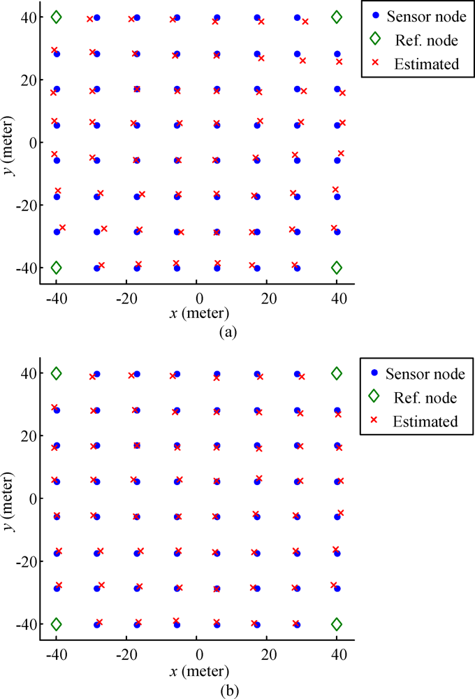
 ) and estimated coordinate (white cross ×) of the sensor node.
) and estimated coordinate (white cross ×) of the sensor node.
) and estimated coordinate (white cross ×) of the sensor node.


| Simulation Parameters | Parameter Value |
|---|---|
| Size of sensor field | 80 m × 80 m |
| Number of grids | 8 |
| Number of reference nodes | 4 |
| Path-loss exponent α | 3 |
| Standard deviation of noise in Ω<r, s>(δ) | 6 dB |
| First meter (d0 = 1) RSS P0 | −30 dBm |
| RSS detection threshold | −80 dBm |
| Neighborhood selection threshold | −75 dBm |
| Method | Bias (m) | STD (m) | RMSE (m) |
|---|---|---|---|
| MDS(W1) | 8.40 | 15.26 | 17.41 |
| MDS(W2) | 12.23 | 10.96 | 16.42 |
| MDS(W3) | 9.18 | 10.97 | 14.30 |
| MDS(W4) | 9.03 | 12.8 | 15.67 |
| MLE | 6.81 | 13.56 | 15.18 |
| MDS(W1)-MLE | 5.93 | 12.39 | 13.73 |
| MDS(W2)-MLE | 5.44 | 9.06 | 10.57 |
| MDS(W3)-MLE | 4.68 | 8.89 | 10.05 |
| MDS(W4)-MLE | 5.19 | 9.96 | 11.24 |
| Proposed Method (1 cycle) | 1.89 | 1.31 | 3.75 |
| Proposed Method (2 cycle) | 1.30 | 0.66 | 2.43 |
©2010 by the authors; licensee Molecular Diversity Preservation International, Basel, Switzerland. This article is an open access article distributed under the terms and conditions of the Creative Commons Attribution license (http://creativecommons.org/licenses/by/3.0/)
Share and Cite
Jiang, J.-A.; Chuang, C.-L.; Lin, T.-S.; Chen, C.-P.; Hung, C.-H.; Wang, J.-Y.; Liu, C.-W.; Lai, T.-Y. Collaborative Localization in Wireless Sensor Networks via Pattern Recognition in Radio Irregularity Using Omnidirectional Antennas. Sensors 2010, 10, 400-427. https://doi.org/10.3390/s100100400
Jiang J-A, Chuang C-L, Lin T-S, Chen C-P, Hung C-H, Wang J-Y, Liu C-W, Lai T-Y. Collaborative Localization in Wireless Sensor Networks via Pattern Recognition in Radio Irregularity Using Omnidirectional Antennas. Sensors. 2010; 10(1):400-427. https://doi.org/10.3390/s100100400
Chicago/Turabian StyleJiang, Joe-Air, Cheng-Long Chuang, Tzu-Shiang Lin, Chia-Pang Chen, Chih-Hung Hung, Jiing-Yi Wang, Chang-Wang Liu, and Tzu-Yun Lai. 2010. "Collaborative Localization in Wireless Sensor Networks via Pattern Recognition in Radio Irregularity Using Omnidirectional Antennas" Sensors 10, no. 1: 400-427. https://doi.org/10.3390/s100100400