A Focusing Method in the Calibration Process of Image Sensors Based on IOFBs


Abstract
:1. Introduction
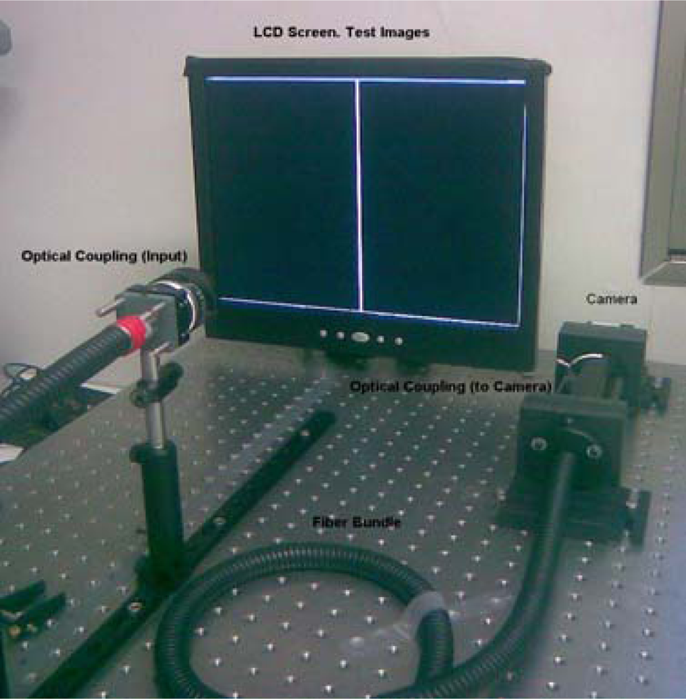
- An LCD monitor, which acts as a light source in FDDT, illuminating the IOFB homogenously. This element is used in calibration to project a serial image of known patterns onto the IOFB entrance.
- A PC or similar unit to control and process the images emitted by the sensor.
- A CMOS camera, which acts as a sensor and is controlled by the PC, for capturing images of the IOFB output face.
- Several additional accessories, including the lens couplers.
- An IOFB, which acts as a transport element.
- Location of fibers on the outside face of an IOFB. These locations are the first elements included on the Lookup Table (LUT) as output parameters, where the captured input information is redistributed.
- A reduced number of coordinates to process in bundle calibration and decoding process is required.
- Fiber response can be particularized if each one is stimulated homogenously.
2. Background
3. Proposed Focusing Measures Process
- Content-independent: it should not be influenced by any particular structure in the image, such as brighter points, etc.
- Monoticity: it should decrease monotonically above and below the focus position
- Good power of discrimination and accuracy: it should give a sharper response when the focus point is closer. The sharper the focus, the easier it is to focus the system accurately. The focus value should be able to combat the effect of noise and low-contrast imaging conditions.
- Applicability: it should work well for any reasonable sample and conditions.
- Implementation: it should be easy to implement and efficient.
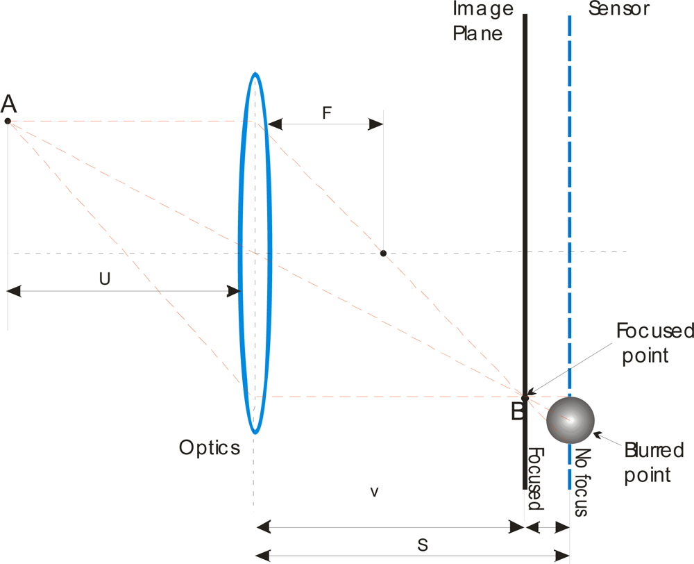
3.1. Focusing Model for an Incoherent Fiber Bundle
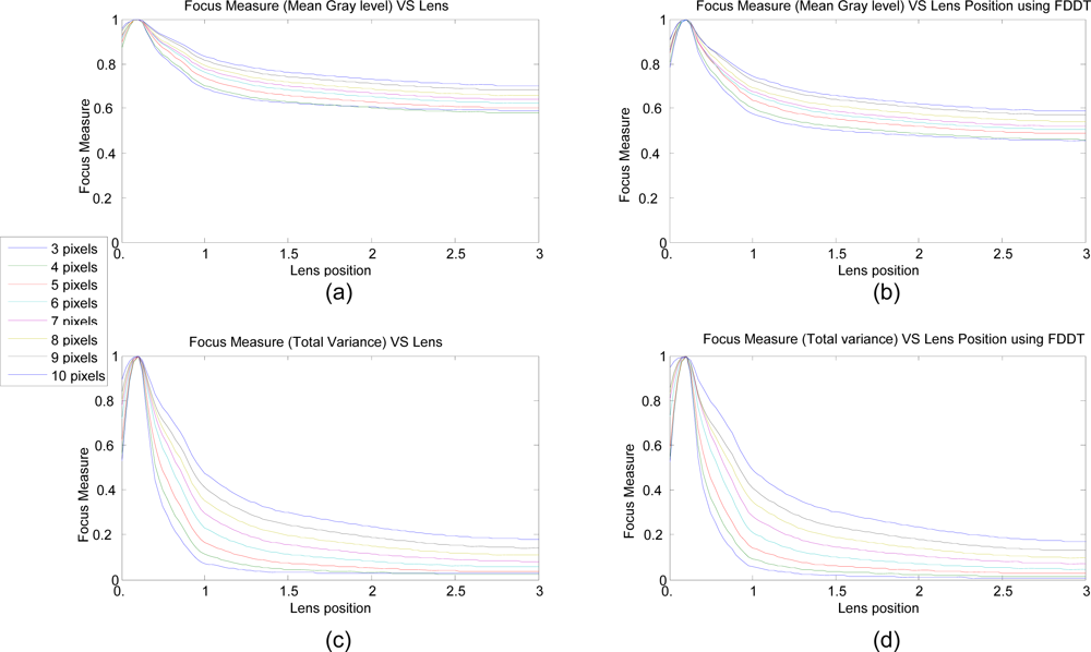
4. Focusing Results
5. Conclusions
Acknowledgments
References
- Fernandez, P.R.; Lazaro, J.L.; Gardel, A.; Esteban, O.; Cano, A.E.; Revenga, P.A. Location of Optical Fibers for the Calibration of Incoherent Optical Fiber Bundles for Image Transmission. IEEE Instrum. Meas. Trans 2009, 58, 2996–3003. [Google Scholar]
- Lázaro, J.L.; Fernández, P.R.; Gardel, A.; Cano, A.E.; Luna, C.A. Calibration of Sensor Based on IOFB Used For Remote Image Transmission. Sensors 2009, 9, 8215–8229. [Google Scholar]
- Yap, P.T.; Raveendran, P. Image Focus Measure Based on Chebyshev Moments. IEE Proc.—Vis. Image Signal Pro 2004, 151, 128–136. [Google Scholar]
- Wu, S.; Lin, W.; Jiang, L.; Xiong, W. An Objective Out-of-Focus Blur Measurement. Information, Communications and Signal Processing, 2005 Fifth International Conference on ICICS, Bangkok, Thailand, 2005; pp. 334–338.
- Subbarao, M.; Tyan, J. Selecting the Optimal Focus Measure for Autofocusing and Depth-from-Focus. IEEE Trans. Patt. Anal. Mach. Int 1998, 20, 864–870. [Google Scholar]
- Shen, C.; Chen, H. Robust focus Measure for Low-Contrast Images. IEEE International Conference on Consumer Electronics, ICCE’06, Las Vegas, NM, USA, 2006; pp. 69–70.
- Sezan, M.I.; Pavlovic, G.; Murat, A.; Tanju, A. On Modelling the Focus Blur in Image Restoration. IEEE Acoustics, Speech, and Signal Processing, International Conference on ICASSP-91, Toronto, Ont., Canada, 1991; 4, pp. 2485–2488.
- Subbarao, M.; Tyan, J. The optimal Focus Measure for Passive Autofocusing and Depth-from-Focus. Proceedings of SPIE Conference Viedometrics IV, Philadelphia, PA, USA, 1995; 2, pp. 89–99.
- Subbarao, M.; Choi, T.; Nikzad, A. Focusing Techniques. J. Opt. Eng 1993, 32, 2824–2836. [Google Scholar]
- Tsai, T.; Lin, C. A New Auto-Focus Method Based on Focal Window Searching and Tracking Approach for Digital Camera. Communications, Control and Signal Processing, ISCCSP 2008. 3rd International Symposium, St. Julians, Malta, 2008; pp. 650–653.


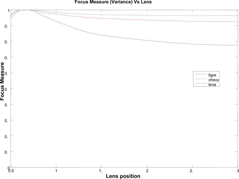
| File | Chevrolet | Lena | Tiger |
|---|---|---|---|
| Lens Posit. | |||
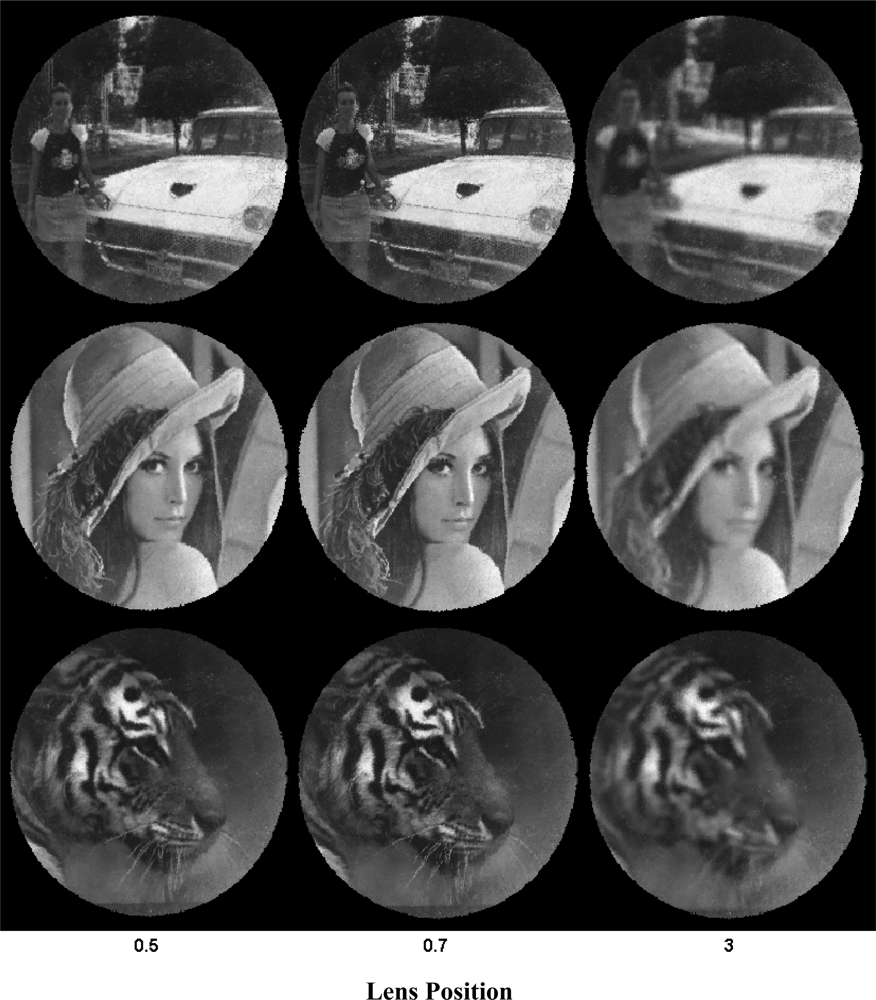
| 0.5 | 0.87809 | 0.90179 | 0.79068 |
| 0.6 | 0.89811 | 0.9265 | 0.84814 |
| 0.7 | 0.92416 | 0.94232 | 0.86918 |
| 0.85 | 0.91523 | 0.93729 | 0.85346 |
| 1.0 | 0.90773 | 0.93455 | 0.838 |
| 1.5 | 0.89771 | 0.93013 | 0.81185 |
| 3.0 | 0.89549 | 0.92973 | 0.80978 |
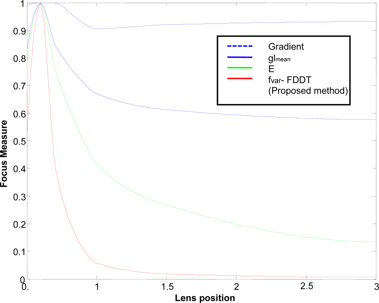
| Measure | Q |
|---|---|
| Gradient | 0.2750 |
| glmean | 0.1850 |
| Image energy E | 0.1500 |
| fvar using FDDT (proposed method) | 0.0750 |
©2010 by the authors; licensee Molecular Diversity Preservation International, Basel, Switzerland. This article is an open access article distributed under the terms and conditions of the Creative Commons Attribution license (http://creativecommons.org/licenses/by/3.0/)
Share and Cite
Fernández, P.R.; Lázaro, J.L.; Gardel, A.; Cano, Á.E.; Bravo, I. A Focusing Method in the Calibration Process of Image Sensors Based on IOFBs. Sensors 2010, 10, 47-60. https://doi.org/10.3390/s100100047
Fernández PR, Lázaro JL, Gardel A, Cano ÁE, Bravo I. A Focusing Method in the Calibration Process of Image Sensors Based on IOFBs. Sensors. 2010; 10(1):47-60. https://doi.org/10.3390/s100100047
Chicago/Turabian StyleFernández, Pedro R., José L. Lázaro, Alfredo Gardel, Ángel E. Cano, and Ignacio Bravo. 2010. "A Focusing Method in the Calibration Process of Image Sensors Based on IOFBs" Sensors 10, no. 1: 47-60. https://doi.org/10.3390/s100100047