Automatic Chessboard Detection for Intrinsic and Extrinsic Camera Parameter Calibration


Abstract
:
1. Introduction
2. Related Work
- Since the process is mechanical, users commonly do not pay sufficient attention to the process, and as a result it is subject to errors that are difficult to detect.
- The number of applications is constantly growing and there are many fields of research that use a large number of cameras, thus emphasizing the need for more automatic calibration processes.
- Although the calibration of the camera intrinsic parameters is only carried out once, this is not the case for the extrinsic parameters, which may change on various occasions until the definitive configuration is obtained.
- Up until now, the steps required for the correct calibration process have been carried out by trained and experienced personnel who are familiar with the selection of adequate positions on the patterns, but this situation has to change if such applications are to be performed by users with no specific training in Computer Vision.
3. Board Detection
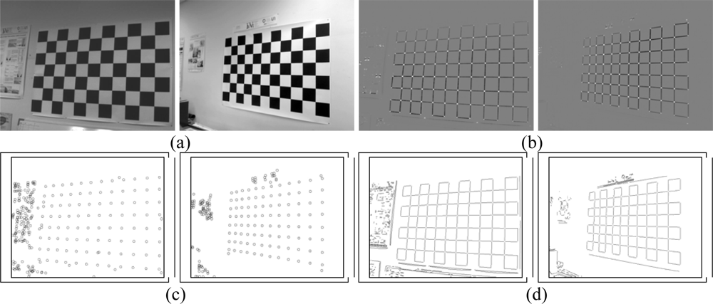
3.1. Corner detection
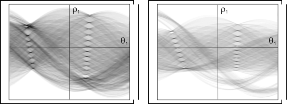
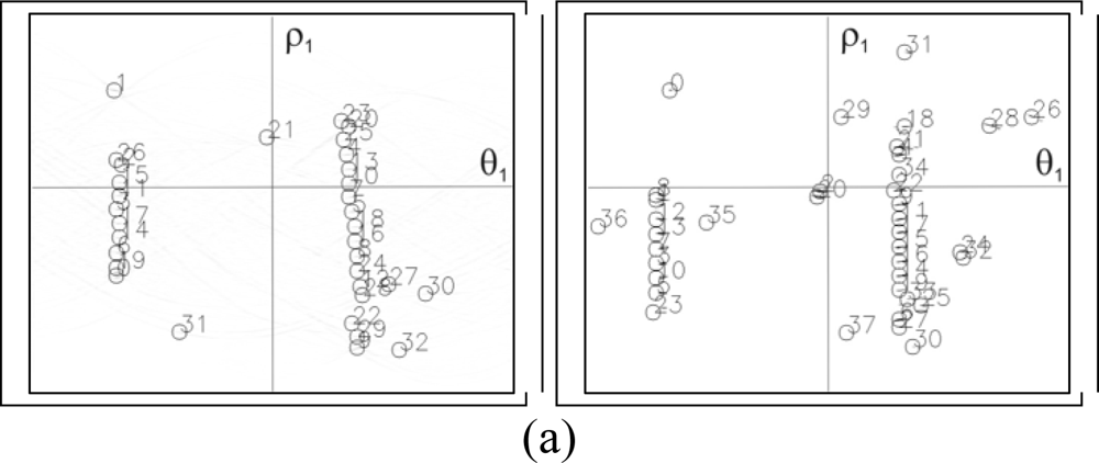
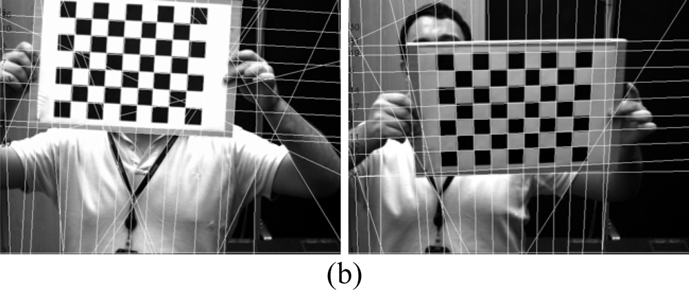
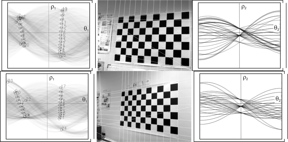
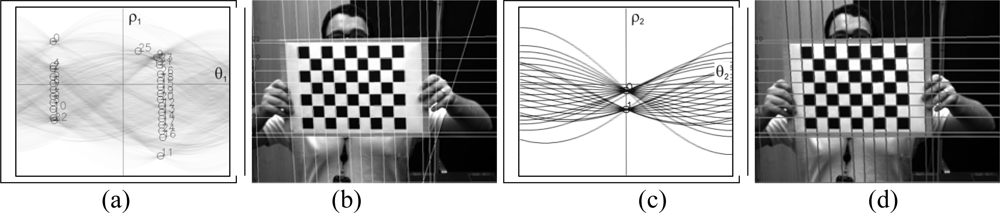
3.2. Hough Transform
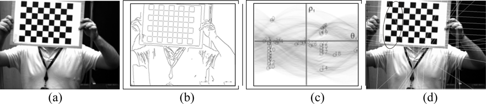
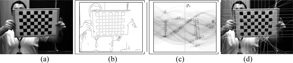
3.3. Determination of the set of lines
3.4. Pattern localization
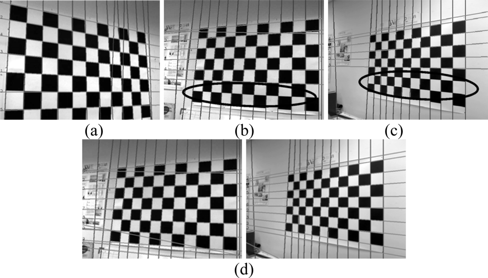
- The external lines that outline the board consist of lines where only half of the squares provide points for the Hough transform, these lines are not always detected. If a robust detection system is required involving different positions and conditions an element whose detection is uncertain should not be added. Even though this problem can be solved the following reason advises against its use.
- The detection of the board serves for the detection of corners, the edge of this pattern is where the corners are most poorly defined; this is because there are no alternating black and white squares in both directions, which is the case for the rest of the corners. For this reason they are not considered as good points to be used in the calibration process.
3.5. Calibration of the extrinsic parameters
4. Results
5. Conclusions
Acknowledgments
References and Notes
- VISION. Comunicaciones de Video de Nueva Generacion. Availalbe online: www.cenit-vision.org/index.php (accessed on 10 March 2010).
- Trucco, E.; Verri, A. Introductory Techniques for 3-D Computer Vision; Prentice Hall: Englewood Cliffs, NJ, USA, 1998. [Google Scholar]
- Ronda, J.I.; Valdés, A.; Gallego, G. Line geometry and camera autocalibration. J. Math. Imaging Vision 2008, 32, 193–214. [Google Scholar]
- Zhang, Z. Camera calibration with one-dimensional objects. IEEE Trans. Pattern Anal. Mach. Intell 2004, 26, 892–899. [Google Scholar]
- Grammatikopoulos, L.; Karras, G.; Petsa, E.; Kalisperakis, I. A unified approach for automatic camera calibration from vanishing points. Int. Arch. Photogram. Remote Sens. Spatial Inf. Sci 2006, XXXVI. Part 5.. [Google Scholar]
- Zhaoxue, C.; Pengfei, S. Efficient method for camera calibration in traffic scenes. Electron. Lett 2004, 40, 368–369. [Google Scholar]
- Zhang, Z. A fexible new technique for camera calibration. IEEE Trans. Pattern Anal. Mach. Intell 2000, 11, 1330–1334. [Google Scholar]
- Bouguet, J.Y. Camera calibration toolbox for Matlab. Available online: www.vision.caltech.edu/bouguetj/calib_doc (accessed on 10 March 2010).
- Strobl, K.H.; Sepp, W.; Fuchs, S.; Paredes, C.; Arbter, K. DLR CalDe and DLR CalLab; Institute of Robotics and Mechatronics, German Aerospace Center (DLR): Oberpfaffenhofen, Germany; Available online: www.robotic.dlr.de/callab (accessed on 10 March 2010).
- Bradski, G.; Kaehler, A. Learning OpenCV: Computer Vision with the OpenCV Library. O’Reilly: Sebastopol, CA, USA, 2008. [Google Scholar]
- Fiala, M.; Shu, C. Self-identifying patterns for plane-based camera calibration. Mach. Vis. Appl 2008, 19, 209–216. [Google Scholar]
- Ahn, S.J.; Rauh, W.; Kim, S.I. Circular coded target for automation of optical 3D-measurement and camera calibration. Int. J. Pattern Recogn. Artif. Intell 2001, 15, 905–919. [Google Scholar]
- Forbes, K.; Voight, A.; Bodika, N. An inexpensive automatic and accurate camera calibration method. Proceedings of the Thirteenth Annual Symposium of the Pattern Recognition Association of South Africa, Langebaan, South Africa, November 28–29, 2002.
- Matas, J.; Soh, L.M.; Kittler, J. Object recognition using a tag. Proceedings of the International Conference on Image Processing, Washington, DC, USA, October 26–29, 1997; pp. 877–880.
- Tsai, R.Y. A versatile camera calibration technique for high-accuracy 3D machine vision metrology using off-the-shelf TV cameras and lenses. J. Rob. Autom 1987, 3, 323–344. [Google Scholar]
- Shu, C.; Brunton, A.; Fiala, M. Automatic Grid Finding in Calibration Patterns Using Delaunay Triangulation; Technical Report NRC-46497/ERB-1104; National Research Council, Institute for Information Technology: Ottawa, Ontario, Canada, 2003. [Google Scholar]
- Harris, C.; Stephens, M.J. A combined corner and edge detector. Proceedings of the Fourth Alvey Vision Conference, Manchester, UK, August 31–September 2, 1988; pp. 147–152.
- Yu, C.; Peng, Q. Robust recognition of checkerboard pattern for camera calibration. Opt. Eng 2006, 45, 093201. [Google Scholar]
- Wang, Z.; Wu, W.; Xu, X.; Xue, D. Recognition and location of the internal corners of planar checkerboard calibration pattern image. Applied Math. Comput 2007, 185, 894–906. [Google Scholar]
- Douskos, V.; Kalisperakis, I.; Karras, G. Automatic calibration of digital cameras using planar chess-board patterns. Proceedings of the 8th Conference on Optical 3-D Measurement Techniques, ETH Zurich, Switzerland, July 9–12, 2007; 1, pp. 132–140.
- Douskos, V.; Kalisperakis, I.; Karras, G.; Petsa, E. Fully automatic camera calibration using regular planar patterns. Int. Arch. Photogram. Remote Sens. Spatial Inf. Sci 2008, 37, 21–26. [Google Scholar]
- Ha, J.E. Automatic detection of chessboard and its applications. Opt. Eng 2009, 48, 067205. [Google Scholar]


| fx (px) | fy (px) | cx (px) | cy (px) | Radial distortion | Tangential distortion | Error x (px) | Error y (px) | ||||
|---|---|---|---|---|---|---|---|---|---|---|---|
| k1 10−3 | k2 10−3 | p1 10−3 | p2 10−3 | ||||||||
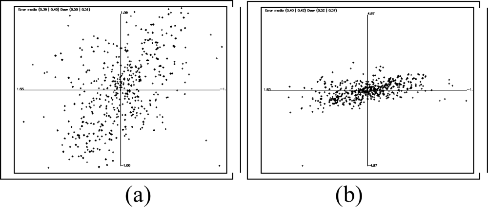
| S1 | Bouguet | 821.1 | 812.8 | 327.4 | 234.6 | −248.5 | 214.9 | 2.5 | −5.1 | 0.50 | 0.36 |
| Our method | 820.6 | 812.4 | 327.4 | 234.7 | −247.0 | 210.9 | 2.5 | −5.1 | 0.39 | 0.40 | |
| S2 | Bouguet | 514.3 | 515.9 | 322.1 | 243.0 | 23.9 | −157.5 | 3.1 | 1.5 | 0.30 | 0.17 |
| Our method | 517.3 | 518.8 | 320.6 | 239.8 | 3.1 | −54.4 | 1.4 | 0.7 | 0.24 | 0.23 | |
| S3 | Bouguet | 2371.6 | 2421.8 | 326.3 | 389.8 | −35.7 | 684.7 | −3.96 | −57.5 | 1.17 | 0.31 |
| Our method | 2440.0 | 2493.0 | 328.2 | 387.9 | 28.0 | 334.9 | −4.2 | −59.5 | 0.93 | 0.39 | |
© 2010 by the authors; licensee Molecular Diversity Preservation International, Basel, Switzerland. This article is an open access article distributed under the terms and conditions of the Creative Commons Attribution license (http://creativecommons.org/licenses/by/3.0/).
Share and Cite
De la Escalera, A.; Armingol, J.M. Automatic Chessboard Detection for Intrinsic and Extrinsic Camera Parameter Calibration. Sensors 2010, 10, 2027-2044. https://doi.org/10.3390/s100302027
De la Escalera A, Armingol JM. Automatic Chessboard Detection for Intrinsic and Extrinsic Camera Parameter Calibration. Sensors. 2010; 10(3):2027-2044. https://doi.org/10.3390/s100302027
Chicago/Turabian StyleDe la Escalera, Arturo, and Jose María Armingol. 2010. "Automatic Chessboard Detection for Intrinsic and Extrinsic Camera Parameter Calibration" Sensors 10, no. 3: 2027-2044. https://doi.org/10.3390/s100302027