Real Time Speed Estimation of Moving Vehicles from Side View Images from an Uncalibrated Video Camera

Abstract
:1. Introduction
2. Problem Statement, Methodology and Specifications
3. Physical Model of Speed Measurement by a Video Camera
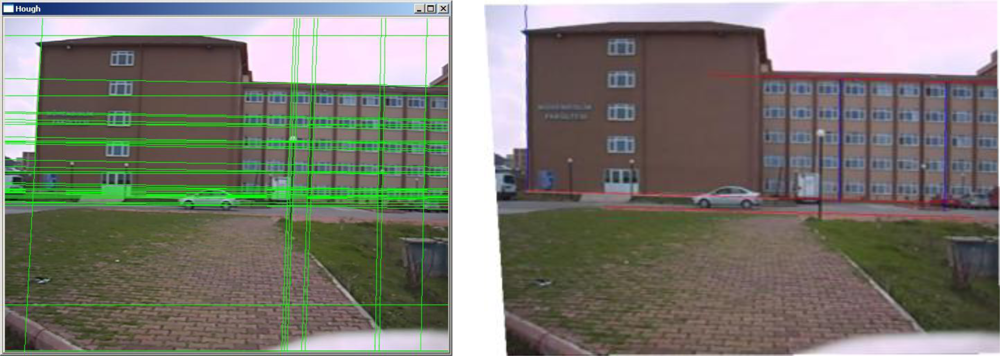
4. Rectification of Frame Images with Vanishing Points
5. Automatic Selection of Points to be Tracked from the Images of the Vehicle
6. Tracking of Selected Points and Estimation of Speed
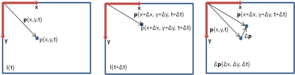
6.1. Optical Flow
6.2. The Lukas-Kanade (LK) Optical Flow Method
7. Conclusions
References
- Cathey, F.W.; Dailey, D.J. A novel technique to dynamically measure vehicle speed using uncalibrated roadway cameras. Proceedings of the IEEE Intelligent Vehicles Symposium, Las Vegas, NV, USA, 6–8 June 2005; pp. 777–782.
- Grammatikopoulos, L.; Karras, G.; Petsa, E. Automatic estimation of vehicle speed from uncalibrated video sequences. Proceedings of the Int. Symposium on Modern Technologies, Education and Professional Practice in Geodesy and Related Fields, Sofia, Bulgaria, 3–4 November 2005; pp. 332–338.
- Melo, J.; Naftel, A.; Bernardino, A.; Victor, J.S. Viewpoint independent detection of vehicle trajectories and lane geometry from uncalibrated traffic surveillance cameras. Proceedings of the International Conference on Image Analysis and Recognition, Porto, Portugal, 29 September–1 October 2004; pp. 454–462.
- Morris, B.; Trivedi, M. Improved vehicle classification in long traffic video by cooperating tracker and classifier modules. Proceedings of the IEEE International Conference on Advanced Video and Signal Based Surveillance, Sydney, Australia, 22–24 November 2006.
- Douxchamps, D.; Macq, B.; Chihara, K. High accuracy traffic monitoring using road-side line scan cameras. Proceedings of the IEEE Intelligent Transportation Systems Conference (ITLS 2006), Toronto, Canada, September 2006; pp. 875–878.
- Gupte, S.; Masaud, O.; Martin, F.K.R.; Papanikolopoulos, N.P. Detection and classification of vehicles. IEEE Trans. Intell. Transp. Syst 2002, 3, 37–47. [Google Scholar]
- Guo, M.; Ammar, M.H.; Zegura, E.W. V3: A vehicle to vehicle live viedo streaming architecture. Pervasive Mob. Comput 2005, 1, 404–424. [Google Scholar]
- Dailey, D.J.; Cathey, F.W.; Pumrin, S. An algorithm to estimate mean traffic speed using uncalibrated cameras. IEEE Trans. Intell. Transp. Syst 2000, 1, 98–107. [Google Scholar]
- Schoepflin, T.N.; Dailey, D.J. Dynamic camera calibration of roadside traffic management cameras for vehicle speed estimation. IEEE Trans. Intell. Transp. Syst 2003, 4, 90–98. [Google Scholar]
- Cucchiara, R.; Grana, C.; Piccardi, M.; Prati, A. Detecting objects, shadows and ghosts in video streams by exploiting colour and motion information. Proceedings of the 11th International Conference on Image Analysis and Processing ICIAP, Palermo, Italy, 26–28 September 2001; pp. 360–365.
- Elgammal, A.; Duraiswami, R. Background and foreground modeling using nonparametric kernel density estimation for visual surveillance. Proc. IEEE 2002, 90, 1151–1163. [Google Scholar]
- Kamijo, S.; Matsushita, Y.; Ikeuchi, M.; Sakauchi, M. Traffic monitoring and accident detection at intersections. IEEE Trans. Intell. Transp. Syst 2000, 1, 108–118. [Google Scholar]
- Koller, D.; Weber, J.; Malik, J. Robust multiple car tracking with occlusion reasoning. Proceeding of the Third European Conference on Computer Vision, Stockholm, Sweden, 1994; pp. 189–196.
- Aghajan, H.; Cavallaro, A. Multi-Camera Networks: Principles and Applications; Academic Press Elsevier Inc: Burlington, MA, USA, 2009. [Google Scholar]
- Bouget, J.Y. Pyramidal Implementation of the Lucas Kanade Feature Tracker Description of the Algorithm; Intel Microprocessor Research Labs: Santa Clara, CA, USA, 2000. [Google Scholar]
- Van Den Heuvel, A.F. Line photogrammetry and its application for reconstruction from a single image. Publikationen der Deutschen Gesellschaft für Photogrammetrie und Fernerkundung 2000, 8, 255–263. [Google Scholar]
- Simond, N.; Rives, P. Homography from a vanishing point in urban scenes. Proceedings of the Intelligent Robots and System, Las Vegas, NV, USA, October 2003; pp. 1005–1010.
- Cipolla, R.; Drummond, T.; Robertson, D. Camera calibration from vanishing points in images of architectural scenes. Proceedings of the 10th British Machine Vision Conference, Nottingham, England, September 1999.
- Grammatikopoulos, L.; Karras, G.E.; Petsa, E. Geometric information from single uncalibrated images of roads. Int. Arch. Photogramm. Remote Sens 2002, 34, 21–26. [Google Scholar]
- Harris, C.; Stephens, M. A Combined corner and edge detector. Proceedings of the 4th Alvey Vision Conference, Manchester, England, 31 August–2 September, 1988; pp. 147–151.
- Bradsky, G.; Kaehler, A. Learning Open CV Computer Vision with the Open CV Library; O’Reilly Media Inc: Sebastopol, CA, USA, 2008. [Google Scholar]
- Shi, J.; Tomasi, C. Good features to track. Proceedings of the 9th IEEE Conference on Computer Vision and Pattern Recognition, Seattle, WA, USA, June 1994; pp. 593–600.
- Lucchese, L.; Mitra, K.S. Using saddle points for subpixel feature detection in camera calibration targets. Proceedings of the 2002 Asia Pacific Conference on Circuits and Systems, Singapore, 16–18 December 2002; pp. 191–195.
- Horn, B.K.P.; Schunck, B.G. Determining optical flow. Artif. Intell 1981, 17, 185–203. [Google Scholar]
- Lucas, B.D.; Kanade, T. An iterative image registration technique with an application to stereo vision. Proceedings of the DARPA Image Understanding Workshop, Washington, USA, June 1981; pp. 121–130.
- Liu, B.S. Association of intersection approach speed with driver characteristics, vehicle type and traffic conditions comparing urban and suburban areas. Accid. Anal. Prevent 2007, 39, 216–223. [Google Scholar]
- Keskin, M.; Say, S.M. Feasibility of low cost GPS receivers for ground speed measurement. Comput. Electron. Agric 2006, 54, 36–43. [Google Scholar]
- Al-Gaadi, K.A. Testing the accuracy of autonomous GPS in ground speed measurement. J. Appl. Sci 2005, 5, 1518–1522. [Google Scholar]


| Step I Operations (performed offline) | Step II Operations (real time operations ) |
|---|---|
|
|
| Real time operation | Computation time (in milliseconds)* | Explanation |
|---|---|---|
| 2.3. Find difference ROI image | < 1.0 | completed in microseconds |
| 2.4. Eliminate background changes with histogram thresholding. | < 1.0 | |
| 2.5. Select tracking points from the foreground (vehicle) image | 10–12 | |
| 2.6. Find corresponding points | 14–16 | |
| 2.7. Rectify the coordinates of the selected and the tracked points | < 1.0 | completed in microseconds |
| 2.8. Compute the velocity vectors | < 1.0 | |
| 2.9. Compute mean and standard deviations of the vectors | < 1.0 | |
| 2.10. Eliminate outlier vectors | < 1.0 | |
| 2.11. Compute the average instantaneous speed of the vehicle | < 1.0 | |
| Total execution time | 29–31 |
| Focal length: 5.9 mm. Fps: 30 | Distance (m) | Max speed (km/h) | Explanation |
| 10 | 75 | ||
| 22.95 | 171 | used in this paper | |
| 26.20 | 196 | ||
| 30 | 224 | ||
| 40 | 300 | ||
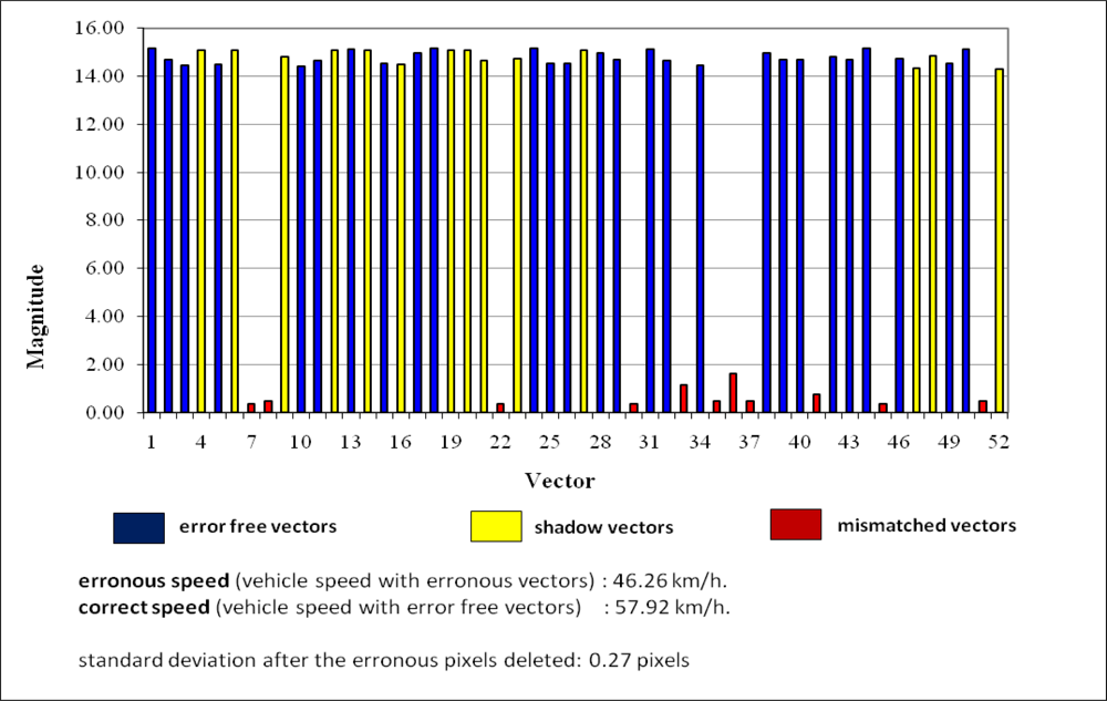
| Vector | Magnitude | Vector | Magnitude | Vector | Magnitude | Vector | Magnitude |
|---|---|---|---|---|---|---|---|
| 1 | 15.17244 | 14 | 15.09534 | 27 | 15.10201 | 40 | 14.67062 |
| 2 | 14.67051 | 15 | 14.53567 | 28 | 14.97215 | 41 | 0.75555 |
| 3 | 14.44615 | 16 | 14.48191 | 29 | 14.67011 | 42 | 14.79012 |
| 4 | 15.09515 | 17 | 14.97209 | 30 | 0.37625 | 43 | 14.67086 |
| 5 | 14.48138 | 18 | 15.17195 | 31 | 15.12538 | 44 | 15.17658 |
| 6 | 15.10202 | 19 | 15.09523 | 32 | 14.63253 | 45 | 0.36652 |
| 7 | 0.367685 | 20 | 15.09504 | 33 | 1.14171 | 46 | 14.73801 |
| 8 | 0.478954 | 21 | 14.64967 | 34 | 14.44434 | 47 | 14.34300 |
| 9 | 14.81166 | 22 | 0.37704 | 35 | 0.47859 | 48 | 14.84108 |
| 10 | 14.42731 | 23 | 14.73827 | 36 | 1.63186 | 49 | 14.52454 |
| 11 | 14.63479 | 24 | 15.17197 | 37 | 0.47909 | 50 | 15.11971 |
| 12 | 15.09527 | 25 | 14.52401 | 38 | 14.97558 | 51 | 0.47341 |
| 13 | 15.11739 | 26 | 14.52534 | 39 | 14.67038 | 52 | 14.29117 |
| Experiment # | Vehicle Direction LR: left to right RL: right to left | Estimated Speed (km/h) | GPS Speed (km/h) | Difference (errors relative to GPS measurements) (km/h) |
|---|---|---|---|---|
| 1 | LR | 38.26 | 38.6 | 0.34 |
| 2 | RL | 36.73 | 38.5 | 1.77 |
| 3 | LR | 37.41 | 38.5 | 1.09 |
| 4 | LR | 47.61 | 48.3 | 0.69 |
| 5 | RL | 57.92 | 57.7 | −0.22 |
| 6 | LR | 57.50 | 57.0 | −0.50 |
| 7 | RL | 64.25 | 63.2 | −1.05 |
| 8 | LR | 68.92 | 67.3 | −1.62 |
| 9 | RL | 75.35 | 76.9 | 1.55 |
© 2010 by the authors; licensee MDPI, Basel, Switzerland. This article is an Open Access article distributed under the terms and conditions of the Creative Commons Attribution license ( http://creativecommons.org/licenses/by/3.0/).
Share and Cite
Doğan, S.; Temiz, M.S.; Külür, S. Real Time Speed Estimation of Moving Vehicles from Side View Images from an Uncalibrated Video Camera. Sensors 2010, 10, 4805-4824. https://doi.org/10.3390/s100504805
Doğan S, Temiz MS, Külür S. Real Time Speed Estimation of Moving Vehicles from Side View Images from an Uncalibrated Video Camera. Sensors. 2010; 10(5):4805-4824. https://doi.org/10.3390/s100504805
Chicago/Turabian StyleDoğan, Sedat, Mahir Serhan Temiz, and Sıtkı Külür. 2010. "Real Time Speed Estimation of Moving Vehicles from Side View Images from an Uncalibrated Video Camera" Sensors 10, no. 5: 4805-4824. https://doi.org/10.3390/s100504805