Optimization of the Sampling Periods and the Quantization Bit Lengths for Networked Estimation

Abstract

This paper is concerned with networked estimation, where sensor data are transmitted over a network of limited transmission rate. The transmission rate depends on the sampling periods and the quantization bit lengths. To investigate how the sampling periods and the quantization bit lengths affect the estimation performance, an equation to compute the estimation performance is provided. An algorithm is proposed to find sampling periods and quantization bit lengths combination, which gives good estimation performance while satisfying the transmission rate constraint. Through the numerical example, the proposed algorithm is verified.

1. Introduction

Recently, networked monitoring systems are becoming increasingly popular, where sensor data are transmitted to a monitoring station through wired or wireless networks [1, 2]. In a monitoring station, estimation algorithms (such as a Kalman filter) are used to estimate the system states. A network between sensor nodes and a monitoring station can induce many problems such as time delays, packet dropouts, and limited bandwidth, where they depend on network types and scheduling methods. We note that the network issue (for example, what kinds of scheduling methods should be used?) itself is a big research area [3]. Also time delays and packet dropouts [4–7] are one of most important problems in networked estimation problems.

In this paper we focus on the case where there are many sensors and the network bandwidth is limited. For example, suppose there are three sensors (A,B,C) and 90 bytes/s can be transmitted over a network. How does one assign 90 bytes/s to each sensor? One method is to assign 30 bytes/s to each sensor. If sensor A monitors fast changing value and sensor B monitors slowly changing value, it might not be the best strategy: more data rate should be assigned to sensor A and the data rate of sensor B should be reduced. These issues are discussed quantitatively in this paper.

Note that the data rate of each sensor depends on the sampling frequency and the quantization bit length. For example, (100 Hz, 8 bit) case and (50 Hz, 16 bit) case have the same data rate (100 bytes/s). Thus given the same data rate, we have many possible combinations of the sampling frequencies and the quantization bit lengths. We first investigate how the sampling frequency and the quantization bit length affect the estimation performance and then propose a method to choose the sampling frequency and the quantization bit length of each sensor.

Using different sampling frequencies for different sensors is discussed in [10], where the sampling frequencies is chosen by minimizing the Kalman filter error covariance. In [11], the sampling frequency assignment algorithm is given, where a sampling frequency is chosen from a finite discrete set. In [12], a similar sampling frequency assignment is considered, where location of sensors and cost of measurement are also considered in the optimization problem. We note there are other attempts, where an event-based transmission method [8, 9] is used instead of a periodic transmission. In this paper, we assume that periodic sampling of sensor data.

Quantization is an extensively studied area [13]. Relating the estimation problem, a logarithm quantizer is proposed in [14]. Although theoretically appealing, the quantizer is applied to the innovation of a filter rather than to an output directly. The effect of quantization can be reduced by treating the quantization error as measurement noises as in [15]. In [16] and [17], quantization bit length assignment algorithms are proposed, where the bit length is computed by minimizing a performance index. The performance index is not directly related to estimation performance (e.g., the filter error covariance).

Simultaneous optimization of the sampling frequency and the quantization bit length has not been reported yet. In this paper, both parameters are selected so that the estimation performance is optimized given the transmission rate constraint.

The paper is organized as follows. In Section 2., estimation performance P is defined, which depends on the sampling periods and quantization bit lengths. In Section 3., a suboptimal algorithm to compute sampling period and quantization bit length combination is proposed. Through numerical examples, the proposed method is verified in Section 4. and conclusion is given in Section 5.

2. Problem Formulation

In this section, estimation performance is defined when the sampling frequency and the quantization bit length of each sensor are given. How to optimize the sampling frequency and the quantization bit length is discussed in Section 3.

Consider a linear time-invariant system given by

$$\begin{array}{lll}\dot{x}(t)\hfill & =\hfill & Ax(t)\hspace{0.17em}+w(t)\hfill \\ y(t)\hfill & =\hfill & Cx(t)\hspace{0.17em}+v(t)\hfill \end{array}$$

(1)

where x ∈ Rⁿ is the state we want to estimate and y ∈ R^p is the measurement. Process noise w(t) and measurement noise υ(t), which are uncorrelated, zero mean white Gaussian random processes, satisfy:

$$\begin{array}{lll}\mathrm{E}\{w(t)w(s)\prime \}\hfill & =\hfill & Q\delta (t-s)\hfill \\ \mathrm{E}\{v(t)v(s)\prime \}\hfill & =\hfill & R\delta (t-s)\hfill \\ \mathrm{E}\{w(t)v(s)\prime \}\hfill & =\hfill & 0\hfill \end{array}$$

where E{·} denotes the mean and Q and R are a process noise covariance and a measurement noise covariance, respectively.

Let T_i be the sampling period of the i-th output and thus the corresponding sampling frequency is 1/T_i. We assume that T_i is an integer multiple of constant T: that is, T_i satisfies the following condition:

$$T_i\hspace{0.17em}=\hspace{0.17em}{M}_{i}T$$

(2)

where M_i is an integer and T is the base sampling period.

Let l_i be the quantization bit length of the i-th output. Let y_max,i be the absolute maximum value of the i-th output: that is,

$$\left|y_{k,i}\right|\hspace{0.17em}\le \hspace{0.17em}{y}_{\mathit{max},i}$$

(3)

where y_k,i is the i-th element of y_k. The index k is used to denote the discrete time index. We assume that the uniform quantizer is used. Let δ_i be the quantization level of the i-th output, which is given by

$${\delta }_i\hspace{0.17em}=\hspace{0.17em}\frac{y_{\mathit{max},i}}{2^{l_i-1}}$$

(4)

Let q_k be the quantization error in y_k, then the following is satisfied

$$\left|q_{k,i}\right|\hspace{0.17em}\le \hspace{0.17em}\frac{{\delta }_i}{2}$$

(5)

where q_k,i is the i-th element of q_k.

Now we are going to model (1) in the discrete time considering the sampling period T_i and the quantization length bit l_i. Assume M_i = 1 (1 ≤ i ≤ p) temporarily:

$$\begin{array}{lll}{x}_{k+1}\hfill & =\hfill & \Phi x_k\hspace{0.17em}+\hspace{0.17em}{w}_k\hfill \\ y_k\hfill & =\hfill & C{x}_k\hspace{0.17em}+\hspace{0.17em}{v}_k\hspace{0.17em}+\hspace{0.17em}{q}_k\hfill \end{array}$$

(6)

where x_k ≜ x(kT), Φ ≜ exp(AT) and y_k is the quantized output of y(kT). Process noise w_k and υ_k are uncorrelated and satisfy

$$\mathrm{E}\{w_k{w}_k^{\prime }\}\hspace{0.17em}=\hspace{0.17em}{Q}_d,\hspace{0.17em}\mathrm{E}\{v_k{v}_k^{\prime }\}\hspace{0.17em}=\hspace{0.17em}R$$

(7)

where

$$Q_d\hspace{0.17em}\triangleq \hspace{0.17em}{\int }_0^T\text{exp}(\mathit{Ar})Q\text{exp}(\mathit{Ar})\prime \hspace{0.17em}\mathit{dr}$$

We treat the quantization error as an additional measurement noise as in (6), which is also considered in [15]. The quantization error q_k is assumed to be uncorrelated with w_k and υ_k. If the uniform distribution is assumed, the covariance is given by

$$\mathrm{E}\{q_k{q}_k^{\prime }\}\hspace{0.17em}=\hspace{0.17em}\Delta \hspace{0.17em}=\hspace{0.17em}\text{Diag}(\frac{{\delta }_1^2}{12},\hspace{0.17em}\cdots ,\hspace{0.17em}\frac{{\delta }_p^2}{12})$$

(8)

Now the temporary assumption (M_i = 1) is removed. The second equation of (6) is no longer true and y_k,i is available if k is an integer multiple of M_i. Let ỹ_k be a collection of all available y_k,i at time k. To define ỹ_k in a more formal way, let {r_k,1, r_k,2, . . ., r_k,pk} be a set of all row numbers of available y_k. Then ỹ_k is given by

$${\tilde{y}}_k\hspace{0.17em}\triangleq \hspace{0.17em}\left[\begin{array}{c}\underset{\_}{y_{k,r_k,1}}\\ \underset{\_}{y_{k,r_{k,2}}}\\ \underset{\_}{\cdots }\\ y_{k,r_{k,p_k}}\end{array}\right]$$

(9)

Similarly υ̃_k and q̃_k can be defined and C̃_k is defined as follows:

$${\tilde{C}}_k\hspace{0.17em}=\hspace{0.17em}\left[\begin{array}{c}\underset{\_}{C_{r_{k,1}}}\\ \underset{\_}{C_{r_{k,2}}}\\ \underset{\_}{\cdots }\\ C_{r_{k,p_k}}\end{array}\right]$$

where C_i is the i-th row of C. Thus the measurement equation at time k is given by

$${\tilde{y}}_k\hspace{0.17em}=\hspace{0.17em}{\tilde{C}}_k{x}_k\hspace{0.17em}+\hspace{0.17em}{\tilde{v}}_k\hspace{0.17em}+\hspace{0.17em}{\tilde{q}}_k$$

(10)

where

$$\begin{array}{lll}\mathrm{E}\{{\tilde{v}}_k{\tilde{v}}_k^{\prime }\}\hfill & =\hfill & {\tilde{R}}_k\hfill \\ \mathrm{E}\{{\tilde{q}}_k{\tilde{q}}_k^{\prime }\}\hfill & =\hfill & {\tilde{\Delta }}_k\hfill \end{array}$$

(11)

R̃_k ∈ R^p_k×p_k is a matrix extracted from R so that R̃_k(i, j) = R(r_k,i, r_k,j). Δ̃_k is defined in the same way.

For example, if M₁ = 1 and M₂ = 2, then ỹ_k and C̃_k are given in

Table 1. ỹ_k and C̃_k example (M₁ = 1 and M₂ = 2)

k	1	2	3	4
ỹk	[yk,1]	$\left[\begin{array}{c}{y}_{k,1}\\ y_{k,2}\end{array}\right]$	[yk,1]	$\left[\begin{array}{c}{y}_{k,1}\\ y_{k,2}\end{array}\right]$
C̃k	[C1]	$\left[\begin{array}{c}{C}_1\\ C_2\end{array}\right]$	[C1]	$\left[\begin{array}{c}{C}_1\\ C_2\end{array}\right]$

. We can see that C̃_k is periodic with the period 2, which is the least common multiple of M₁ = 1 and M₂ = 2.

Generally C̃_k is periodic with the period M, where M is the least common multiple of {M₁, M₂, . . ., M_p}.

Using the first equation of (6) repeatedly b times, we have

$$x_{b+a}\hspace{0.17em}=\hspace{0.17em}{\Phi }^b{x}_a\hspace{0.17em}+\hspace{0.17em}\sum _{i=0}^{b-1}{\Phi }^{b-1-i}{w}_{a+i}$$

(12)

It is known that a periodic system can be transformed into a time-invariant system [18, 19]. From (12) with a = kM and b = M, we have

$$x_{(k+1)M}\hspace{0.17em}=\hspace{0.17em}{\Phi }^M\hspace{0.17em}{x}_{\mathit{kM}}\hspace{0.17em}+\hspace{0.17em}\sum _{i=0}^{M-1}{\Phi }^{M-1-i}{w}_{Mk+i}$$

(13)

Also from (12) with a = kM − j and b = j, we have

$$x_{\mathit{kM}}\hspace{0.17em}=\hspace{0.17em}{\Phi }^j\hspace{0.17em}{x}_{\mathit{kM}-j}\hspace{0.17em}+\hspace{0.17em}\sum _{i=0}^{j-1}{\Phi }^{j-1-i}\hspace{0.17em}{w}_{\mathit{kM}-j+i}$$

(14)

Multiplying Φ^−j, we obtain a backward equation:

$$x_{\mathit{kM}-j}\hspace{0.17em}=\hspace{0.17em}{\Phi }^{-j}\hspace{0.17em}{x}_{\mathit{kM}}\hspace{0.17em}-\hspace{0.17em}\sum _{i=0}^{j-1}{\Phi }^{-1-i}{w}_{\mathit{kM}-j+i}$$

(15)

Let x̄_k, w̄_k ȳ_k, ῡ_k and q̄_k be defined by

$${\overline{x}}_k\hspace{0.17em}\triangleq \hspace{0.17em}{x}_{\mathit{kM}}$$

$$\begin{array}{cc}{\overline{w}}_k\hspace{0.17em}\triangleq \hspace{0.17em}\left[\begin{array}{c}{w}_{\mathit{kM}}\\ w_{\mathit{kM}+1}\\ ⋮\\ w_{\mathit{kM}+M-1}\end{array}\right],& {\overline{y}}_k\hspace{0.17em}\triangleq \hspace{0.17em}\left[\begin{array}{c}{\tilde{y}}_{(k-1)M+1}\\ {\tilde{y}}_{(k-1)M+2}\\ ⋮\\ {\tilde{y}}_{kM}\end{array}\right]\\ {\tilde{v}}_k\hspace{0.17em}\triangleq \hspace{0.17em}\left[\begin{array}{c}{\tilde{v}}_{(k-1)M+1}\\ {\tilde{v}}_{(k-1)M+2}\\ ⋮\\ {\tilde{v}}_{kM}\end{array}\right],& {\overline{q}}_k\hspace{0.17em}\triangleq \hspace{0.17em}\left[\begin{array}{c}{\tilde{q}}_{(k-1)M+1}\\ {\tilde{q}}_{(k-1)M+2}\\ ⋮\\ {\tilde{q}}_{kM}\end{array}\right]\end{array}$$

Combining (13), (15) and (10), we have the following time invariant system:

$$\begin{array}{lll}{\overline{x}}_{k+1}\hfill & =\hfill & \overline{A}{\overline{x}}_k\hspace{0.17em}+\hspace{0.17em}\overline{B}{\overline{w}}_k\hfill \\ \hfill {\overline{y}}_k& =\hfill & \overline{C}{\overline{x}}_k\hspace{0.17em}+\hspace{0.17em}{\overline{v}}_k\hspace{0.17em}+\hspace{0.17em}{\overline{q}}_k\hspace{0.17em}+\hspace{0.17em}\overline{D}{\overline{w}}_{k-1}\hfill \end{array}$$

(16)

where

$$\overline{A}\hspace{0.17em}=\hspace{0.17em}{\Phi }^M$$

$$\overline{B}\hspace{0.17em}\triangleq \hspace{0.17em}\hspace{0.17em}\left[{\Phi }^{M-1}\hspace{0.17em}{\Phi }^{M-2}\hspace{0.17em}\cdots \hspace{0.17em}I\right]$$

$$\overline{C}\hspace{0.17em}\triangleq \hspace{0.17em}\left[\begin{array}{c}{\tilde{C}}_1{\Phi }^{-M+1}\\ {\tilde{C}}_2{\Phi }^{-M+2}\\ ⋮\\ {\tilde{C}}_{M-1}{\Phi }^{-1}\\ {\tilde{C}}_M\end{array}\right]$$

$$\overline{D}\hspace{0.17em}\triangleq \hspace{0.17em}\left[\begin{array}{ccccc}0& {\tilde{C}}_1{\Phi }^{-1}& {\tilde{C}}_1{\Phi }^{-2}& \cdots & {\tilde{C}}_1{\Phi }^{-M+1}\\ 0& 0& {\tilde{C}}_2{\Phi }^{-1}& \cdots & {\tilde{C}}_2{\Phi }^{-M+2}\\ ⋮& ⋮& ⋮& \ddots & ⋮\\ 0& 0& 0& \cdots & {\tilde{C}}_{M-1}{\Phi }^{-1}\\ 0& 0& 0& \cdots & 0\end{array}\right]$$

We will apply a Kalman filter to (16). Note that

$$\mathrm{E}\{{\overline{w}}_k{\overline{w}}_k^{\prime }\}\hspace{0.17em}=\hspace{0.17em}\overline{Q}$$

(17)

where

$$\overline{Q}\hspace{0.17em}=\hspace{0.17em}\text{Diag}(Q_d,\hspace{0.17em}{Q}_d,\hspace{0.17em}\cdots ,\hspace{0.17em}{Q}_d,\hspace{0.17em}{Q}_d)$$

$$\mathrm{E}\{({\overline{v}}_k\hspace{0.17em}+\hspace{0.17em}{\overline{q}}_k+\hspace{0.17em}\overline{D}{\overline{w}}_{k-1})\hspace{0.17em}({\overline{v}}_k\hspace{0.17em}+\hspace{0.17em}{\overline{q}}_k\hspace{0.17em}+\hspace{0.17em}\overline{D}{\overline{w}}_{k-1})\prime \}\hspace{0.17em}=\hspace{0.17em}\overline{R}$$

(18)

where

$$\begin{array}{lll}\overline{R}\hfill & =\hfill & \text{Diag}({\tilde{R}}_1,\hspace{0.17em}\cdots ,\hspace{0.17em}{\tilde{R}}_M)\hspace{0.17em}+\hspace{0.17em}\overline{\Delta }\hspace{0.17em}+\hspace{0.17em}\overline{D}\overline{Q}\overline{D}\prime \hfill \\ \overline{\Delta }\hfill & =\hfill & \text{Diag}({\tilde{\Delta }}_1,\hspace{0.17em}\cdots ,\hspace{0.17em}{\tilde{\Delta }}_M).\hfill \end{array}$$

$$\mathrm{E}\{\overline{B}{\overline{w}}_{k-1}\hspace{0.17em}({\overline{v}}_k^{\prime }\hspace{0.17em}+\hspace{0.17em}{\overline{q}}_k^{\prime }\hspace{0.17em}+\hspace{0.17em}(\overline{D}{\overline{w}}_{k-1})\prime )\}\hspace{0.17em}=\hspace{0.17em}\overline{M}\hspace{0.17em}=\hspace{0.17em}\overline{B}\overline{Q}\overline{D}\prime$$

(19)

It is standard to apply a Kalman filter to (16) using (17), (18) and (19): the measurement update and the time update equations are given as follows [20]:

• measurement update

  $$\begin{array}{l}{K}_k\hspace{0.17em}=\hspace{0.17em}(P_k^{-}\overline{C}\prime \hspace{0.17em}+\hspace{0.17em}\overline{M})\hspace{0.17em}(\overline{C}{P}_k^{-}\overline{C}\prime \hspace{0.17em}+\hspace{0.17em}\overline{R}\hspace{0.17em}+\hspace{0.17em}\overline{C}\overline{M}\\ \hspace{0.17em}\hspace{0.17em}\hspace{0.17em}\hspace{0.17em}\hspace{0.17em}\hspace{0.17em}\hspace{0.17em}\hspace{0.17em}\hspace{0.17em}\hspace{0.17em}\hspace{0.17em}\hspace{0.17em}\hspace{0.17em}\hspace{0.17em}+\hspace{0.17em}\overline{M}\prime \overline{C}\prime {)}^{-1}\end{array}$$

  $$P_k\hspace{0.17em}=\hspace{0.17em}{P}_k^{-}\hspace{0.17em}-\hspace{0.17em}{K}_k\hspace{0.17em}(\overline{C}{P}_k^{-}\overline{C}\prime \hspace{0.17em}+\hspace{0.17em}\overline{R}\hspace{0.17em}+\hspace{0.17em}\overline{C}\overline{M}\hspace{0.17em}+\hspace{0.17em}\overline{M}\prime \overline{C}\prime )K_k^{\prime }$$
• time update

  $$P_{k+1}^{-}\hspace{0.17em}=\hspace{0.17em}\overline{A}{P}_k\overline{A}\prime \hspace{0.17em}+\hspace{0.17em}\overline{B}\overline{Q}\overline{B}\prime$$

We will use P as an estimation performance, where P is the steady-state value of $P_k^{-}$:

$$P\hspace{0.17em}\triangleq \hspace{0.17em}\underset{k\to \infty }{\text{lim}}\hspace{0.17em}{P}_k^{-}$$

In the steady state, we have $P_{k+1}^{-}\hspace{0.17em}=\hspace{0.17em}{P}_k^{-}\hspace{0.17em}=\hspace{0.17em}P$. Inserting this into the Kalman filter equation, we have the following Riccati equation:

$$\begin{array}{c}P\hspace{0.17em}=\hspace{0.17em}\overline{A}P\overline{A}\prime \hspace{0.17em}-\hspace{0.17em}(\overline{A}P\overline{C}\prime \hspace{0.17em}+\hspace{0.17em}\overline{A}\overline{M})\\ {(\overline{C}P\overline{C}\prime \hspace{0.17em}+\hspace{0.17em}\overline{R}\hspace{0.17em}+\overline{C}\overline{M}\hspace{0.17em}+\hspace{0.17em}\overline{M}\prime \overline{C}\prime )}^{-1}\hspace{0.17em}(\overline{A}P\overline{C}\prime \hspace{0.17em}+\hspace{0.17em}\overline{A}\overline{M})\prime \\ +\hspace{0.17em}\overline{B}\overline{Q}\overline{B}\prime \end{array}$$

(20)

If the sampling period T_i and the quantization bit length l_i are given, the corresponding estimation performance can be computed from (20).

3. T_i and l_i Optimization

In this section, a method to select the sampling period T_i and the quantization bit l_i are proposed. The main trade-off is between the transmission rate and the estimation performance.

The optimization problem can be formulated as follows:

$$\begin{array}{c}{\text{min}}_{T_i,l_i}\hspace{0.17em}\lambda \prime \hspace{0.17em}\text{Diag}\hspace{0.17em}P\\ \text{subject to}\hspace{0.17em}{\Sigma }_{i=1}^p\hspace{0.17em}\frac{l_i}{T_i}\le \hspace{0.17em}{S}_{\mathit{max}}\end{array}$$

(21)

where λ ∈ Rⁿ is a weighting vector. Note that the transmission rate S is given by

$$S\hspace{0.17em}\triangleq \hspace{0.17em}\sum _{i=1}^p\frac{l_i}{T_i}$$

(22)

and S_max is the transmission rate constraint. The transmission rate S is defined as the sum of each sensor data rate without considering packet overhead. When we apply the algorithm to a specific network, the transmission rate S should be modified to take the packet overhead into account.

Note that T_i = M_iT and P depends on M, which is the least common multiple of M₁, . . ., M_p. To make M constant, M_i is assumed to satisfy

$$\begin{array}{c}{M}_i\hspace{0.17em}=\hspace{0.17em}{2}^{m_i}\hspace{0.17em}(m_i\hspace{0.17em}\text{is an integer})\\ m_{i,min}\hspace{0.17em}\le \hspace{0.17em}{m}_i\hspace{0.17em}\le \hspace{0.17em}{m}_{i,\mathit{max}}\end{array}$$

(23)

With this assumption, the least common multiple M of all possible combinations of M_i = 2^m_i is given by

$$M\hspace{0.17em}=\hspace{0.17em}{2}^{{\mathit{max}}_i\left\{m_{i,\mathit{max}}\right\}}$$

We assume l_i satisfies

$$l_{i,\mathit{min}}\hspace{0.17em}\le \hspace{0.17em}{l}_i\hspace{0.17em}\le \hspace{0.17em}{l}_{i,\mathit{max}}$$

(24)

If the number of combinations is small, P can be computed for all possible combinations. For a case that the number is too large, we propose a suboptimal algorithm. The proposed algorithm is based on the following lemma.

Lemma 1 Let P (m₁, l₁, . . ., m_i, l_i, . . ., m_p, l_p) be the solution to (20). With the assumption (23), the following is satisfied.

$$P(m_1,\hspace{0.17em}{l}_1,\hspace{0.17em}\cdots ,\hspace{0.17em}{m}_i\hspace{0.17em}-\hspace{0.17em}1,\hspace{0.17em}{l}_i,\hspace{0.17em}\cdots ,\hspace{0.17em}{m}_p,\hspace{0.17em}{l}_p)\hspace{0.17em}\le \hspace{0.17em}P(m_1,\hspace{0.17em}{l}_1,\hspace{0.17em}\cdots ,\hspace{0.17em}{m}_i,\hspace{0.17em}{l}_i,\hspace{0.17em}\cdots ,\hspace{0.17em}{m}_p,\hspace{0.17em}{l}_p)$$

(25)

$$P(m_1,\hspace{0.17em}{l}_1,\hspace{0.17em}\cdots ,\hspace{0.17em}{m}_i,\hspace{0.17em}{l}_i\hspace{0.17em}+\hspace{0.17em}1,\hspace{0.17em}\cdots ,\hspace{0.17em}{m}_p,\hspace{0.17em}{l}_p)\hspace{0.17em}\le \hspace{0.17em}P(m_1,\hspace{0.17em}{l}_1,\hspace{0.17em}\cdots ,\hspace{0.17em}{m}_i,\hspace{0.17em}{l}_i,\hspace{0.17em}\cdots ,\hspace{0.17em}{m}_p,\hspace{0.17em}{l}_p)$$

(26)

$$P(m_1,\hspace{0.17em}{l}_1,\hspace{0.17em}\cdots ,\hspace{0.17em}{m}_i\hspace{0.17em}-\hspace{0.17em}1,\hspace{0.17em}{l}_i\hspace{0.17em}+\hspace{0.17em}1,\hspace{0.17em}\cdots ,\hspace{0.17em}{m}_p,\hspace{0.17em}{l}_p)\hspace{0.17em}\le \hspace{0.17em}P(m_1,\hspace{0.17em}{l}_1,\hspace{0.17em}\cdots ,\hspace{0.17em}{m}_i,\hspace{0.17em}{l}_i,\hspace{0.17em}\cdots ,\hspace{0.17em}{m}_p,\hspace{0.17em}{l}_p)$$

(27)

Proof: We will prove with a simple case with m₁ = 0 m₂ = 0, T = 1, M = 2, and p = 2: note that T₁ = 2^m₁T = T and T₂ = 2^m₂T = T. C̄ for m₁ = 0 and m₂ = 0 is given by

$${\overline{C}}_{m_1=0,m_2=0}\hspace{0.17em}=\hspace{0.17em}\left[\left[\begin{array}{c}{C}_1\\ C_2\\ C_1\\ C_2\end{array}\right]\right]$$

The subscript (m₁ = 0, m₂ = 0) is used to emphasize that m₁ = 0 and m₂ = 0. Also let R̄_m1=0,m2=0 be R̄ defined in (18) and P(0, l₁, 0, l₂) be a solution to (20) when m₁ = 0 and m₂ = 0.

Now consider a case with m₁ = 0 and m₂ = 1 Instead of computing P(0, l₁, 1, l₂) using (20) with C̄_m1=0,m2=1, we can compute P(0, l₁, 1, l₂) using (20) with m₁ = 0 and m₂ = 0 except that R̄_m1=0,m2=0 is replaced by R̄_modified, which is defined by

$${\overline{R}}_{\mathit{modified}}\hspace{0.17em}=\hspace{0.17em}{\overline{R}}_{(m_1=0,m_2=0})\hspace{0.17em}+\hspace{0.17em}\text{Diag}(0,\infty ,0,0).$$

Note that adding ∞ to the (2, 2) element of R̄_m1=0,m2=0 is equivalent to ignoring the second output of y_k when k is an integer multiple of 2. Thus P(0, l₁, 1, l₂) computed in this way is the estimation error covariance when m₁ = 0 and m₂ = 1. Since R̄_modified ≥ R̄, we have from the monotonicity of the Riccati equation (see Corollary 5.2 in [21])

$$P(0,\hspace{0.17em}{l}_1,\hspace{0.17em}0,\hspace{0.17em}{l}_2)\hspace{0.17em}\le \hspace{0.17em}P(0,\hspace{0.17em}{l}_1,\hspace{0.17em}1,\hspace{0.17em}{l}_2)$$

The general case for (25) can be proved similarly.

Proving the second inequality is more straightforward from the monotonicity of the Riccati equation [21] and from the fact

$${\overline{R}}_{(m_1,l_1,\cdots ,m_i,l_i+1,\cdots ,m_p,l_p})\hspace{0.17em}\le \hspace{0.17em}{\overline{R}}_{(m_1,l_1,\cdots ,m_i,l_i,\cdots ,m_p,l_p)}$$

The third inequality (27) is just a combination of (25) and (26):

$$\begin{array}{c}P(m_1,\hspace{0.17em}{l}_1,\hspace{0.17em}\cdots ,\hspace{0.17em}{m}_i\hspace{0.17em}-1,\hspace{0.17em}{l}_i\hspace{0.17em}+\hspace{0.17em}1,\hspace{0.17em}\cdots ,\hspace{0.17em}{m}_p,\hspace{0.17em}{l}_p)\hspace{0.17em}\le \hspace{0.17em}P(m_1,\hspace{0.17em}{l}_1,\hspace{0.17em}\cdots ,\hspace{0.17em}{m}_i,\hspace{0.17em}{l}_i\hspace{0.17em}+\hspace{0.17em}1,\hspace{0.17em}\cdots ,\hspace{0.17em}{m}_p,\hspace{0.17em}{l}_p)\\ \le \hspace{0.17em}P(m_1,\hspace{0.17em}{l}_1,\hspace{0.17em}\cdots ,\hspace{0.17em}{m}_i,\hspace{0.17em}{l}_i,\hspace{0.17em}\cdots ,\hspace{0.17em}{m}_p,\hspace{0.17em}{l}_p)\end{array}$$

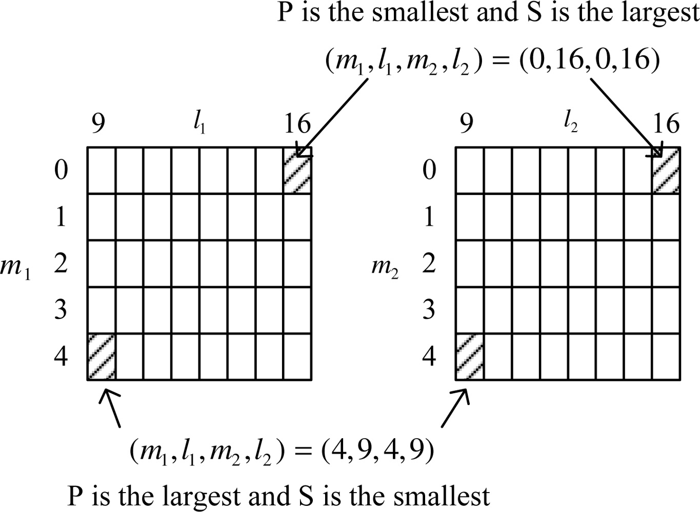
To explain Lemma 1, we consider a simple example with the following parameters:

$$\begin{array}{c}p=2\\ m_{1,\mathit{min}}\hspace{0.17em}=\hspace{0.17em}{m}_{2,\mathit{min}}\hspace{0.17em}=\hspace{0.17em}0,\hspace{0.17em}{m}_{1,\mathit{max}}\hspace{0.17em}=\hspace{0.17em}{m}_{2,\mathit{max}}\hspace{0.17em}=\hspace{0.17em}4\\ l_{1,\mathit{min}}\hspace{0.17em}=\hspace{0.17em}{l}_{2,\mathit{min}}\hspace{0.17em}=\hspace{0.17em}9,\hspace{0.17em}{l}_{1,\mathit{max}}\hspace{0.17em}=\hspace{0.17em}{l}_{2,\mathit{max}}\hspace{0.17em}=\hspace{0.17em}16\end{array}$$

(28)

There are 5 × 8 × 5 × 8 = 1, 600 possible combinations (see Figure 1). Using the result in Lemma 1, we know that P is the smallest when (m₁, l₁, m₂, l₂) = (0, 16, 0, 16) and the largest when (m₁, l₁, m₂, l₂) = (4, 9, 4, 9). On the other hand, the transmission rate S is the largest when (m₁, l₁, m₂, l₂) = (0, 16, 0, 16) and the smallest when (m₁, l₁, m₂, l₂) = (4, 9, 4, 9). Note that m_i − 1 and l_i + 1 in Lemma 1 corresponds to the upper and right combination of (m_i, l_i), respectively. Thus as we move the combination from the left-bottom corner toward the right-top corner, λ′P becomes smaller while the transmission rate increases.

In the proposed algorithm, we start from the left-bottom corner combination and move the combination toward the right-top corner combination while the transmission constrained is satisfied. The proposed algorithm is stated in pseudo-codes.

• (m_i, l_i) = (m_i,max, l_i,min), i = 1, . . ., p
• compute λ′P and S
• (P denotes P(m₁, l₁, . . ., m_p, l_p) and S is from (22))
• while (S < S_max)
•   L = { }
•   for i = 1:p
•     if (m_i > m_i,min)
•       L = L ∪ {(m₁, l₁, . . ., m_i − 1, l_i, . . ., m_p, l_p)}
•     if (l_i < l_i,max)
•       L = L ∪ {(m₁, l₁, . . ., m_i, l_i + 1, . . ., m_p, l_p)}
•   end
•   for every element of L, compute G̃_j

  $${\tilde{G}}_j\hspace{0.17em}=\hspace{0.17em}\frac{\lambda \prime P\hspace{0.17em}-\hspace{0.17em}\lambda \prime {\tilde{P}}_j}{{\tilde{S}}_j\hspace{0.17em}-\hspace{0.17em}S}$$

    where P̃_j = P for the j-th element of L
    and S̃_j = S for the j-th element of L
•   (m_i,old, l_i,old) = (m_i, l_i), i = 1, . . ., p
•   Find the maximum of G_j and choose the
    corresponding combination as (m_i, l_i)
•   compute λ′P and S
• end
• Choose the combination (m_i,old, l_i,old)

Note that G̃_j represents the estimation performance improvement per transmission rate increase. For each given (m_i, l_i), we choose (m_i − 1, l_i) and (m_i, l_i + 1) for the next combination candidates. There are at most 2^p combinations. Among the combinations, we find a combination of which G̃_j is the largest. This process is continued until the current transmission rate exceeds S_max.

The number of combinations tested in the proposed algorithm is small compared with the brute force search. For example, the proposed algorithm starts with the top-right-most combination (m₁, l₁, m₂, l₂) = (0, 16, 0, 16) and moves toward bottom-left-most combination (m₁, l₁, m₂, l₂) = (4, 9, 4, 9) at each step until S ≤ S_max is no longer satisfied. Unfortunately, there is no guarantee that the solution found by the proposed method is near the optimal solution. In Section 4., it is shown, however, through a numerical example that the gap between the suboptimal and optimal solution is not large.

We note that the optimization algorithm is applied once when the networked system is designed. Once the sampling period T_i and quantization length l_i are determined, they are programmed in each sensor node. Thus no additional computation is needed in the sensor node.

4. Numerical Example

In this section, the proposed method is verified for the one dimensional attitude estimation problem. The state is defined by

$$x(t)\hspace{0.17em}=\hspace{0.17em}\left[\begin{array}{c}\theta \\ \dot{\theta }\\ \ddot{\theta }\end{array}\right]$$

where θ is the attitude we want to estimate. An accelerometer-based inclinometer and a gyroscope are used as sensors. The system model is given by

$$\begin{array}{l}A\hspace{0.17em}=\hspace{0.17em}\left[\begin{array}{ccc}0& 1& 0\\ 0& 0& 1\\ 0& 0& 0\end{array}\right],\hspace{0.17em}C=\hspace{0.17em}\left[\begin{array}{lll}1\hfill & 0\hfill & 0\hfill \\ 0\hfill & 1\hfill & 0\hfill \end{array}\right]\hfill \\ Q\hspace{0.17em}=\hspace{0.17em}\left[\begin{array}{ccc}0& 0& 0\\ 0& 0& 0\\ 0& 0& 0.2\end{array}\right],\hspace{0.17em}R\hspace{0.17em}=\hspace{0.17em}\left[\begin{array}{cc}0.0056& 0\\ 0& 0.003\end{array}\right]\hfill \end{array}$$

The values given in (28), y_max,1 = 3.1416, y_max,2 = 2.6180 and T = 1 are used.

The optimization problem (21) with S_max = 500 and λ = [1 0 0]′ is considered. λ is a natural choice since we want to estimate θ.

First the optimization problem is solved by a brute force search: all possible combinations are examined. The optimal solution is given by

$$(m_1,\hspace{0.17em}{l}_1,\hspace{0.17em}{m}_2,\hspace{0.17em}{l}_2)\hspace{0.17em}=\hspace{0.17em}(2,\hspace{0.17em}10,\hspace{0.17em}2,\hspace{0.17em}10)$$

and S and λP at the combination are

$$S\hspace{0.17em}=\hspace{0.17em}500,\hspace{0.17em}\lambda P\hspace{0.17em}=\hspace{0.17em}\mathrm{0.00259.}$$

Secondly the proposed suboptimal algorithm is used, where the solution is given by

$$(m_1,\hspace{0.17em}{l}_1,\hspace{0.17em}{m}_2,\hspace{0.17em}{l}_2)\hspace{0.17em}=\hspace{0.17em}(2,\hspace{0.17em}9,\hspace{0.17em}2,\hspace{0.17em}9)$$

and S and λP at the combination are

$$S\hspace{0.17em}=\hspace{0.17em}450,\hspace{0.17em}\lambda P\hspace{0.17em}=\hspace{0.17em}\mathrm{0.00260.}$$

The proposed method was able to find a nearly optimal solution with less computation time. In the brute force search, 479 combinations are tested while 21 combinations are tested in the proposed algorithm.

To test whether the proposed λP is a good indicator of the estimation performance, the data is generated with Matlab and tested with a Kalman filter. The estimation performance is evaluated with the following:

$$P_{\mathit{experiment}}\hspace{0.17em}=\hspace{0.17em}\frac{1}{N}\hspace{0.17em}\sum _{k,1}^N{\theta }_{\mathit{error},k}^2$$

where N is the number of data and θ_error,k = θ − θ̂. Note that θ̂ is computed by [1 0 0] ◯_k. We computed P_experiment for all possible combinations and the minimizing combination is given by

$$(m_1,\hspace{0.17em}{l}_1,\hspace{0.17em}{m}_2,\hspace{0.17em}{l}_2)\hspace{0.17em}=\hspace{0.17em}(2,\hspace{0.17em}9,\hspace{0.17em}2,\hspace{0.17em}10)$$

and S and P_experiment at the combination is

$$S=\hspace{0.17em}475,\hspace{0.17em}{P}_{\mathit{experiment}}\hspace{0.17em}=\hspace{0.17em}0.00159$$

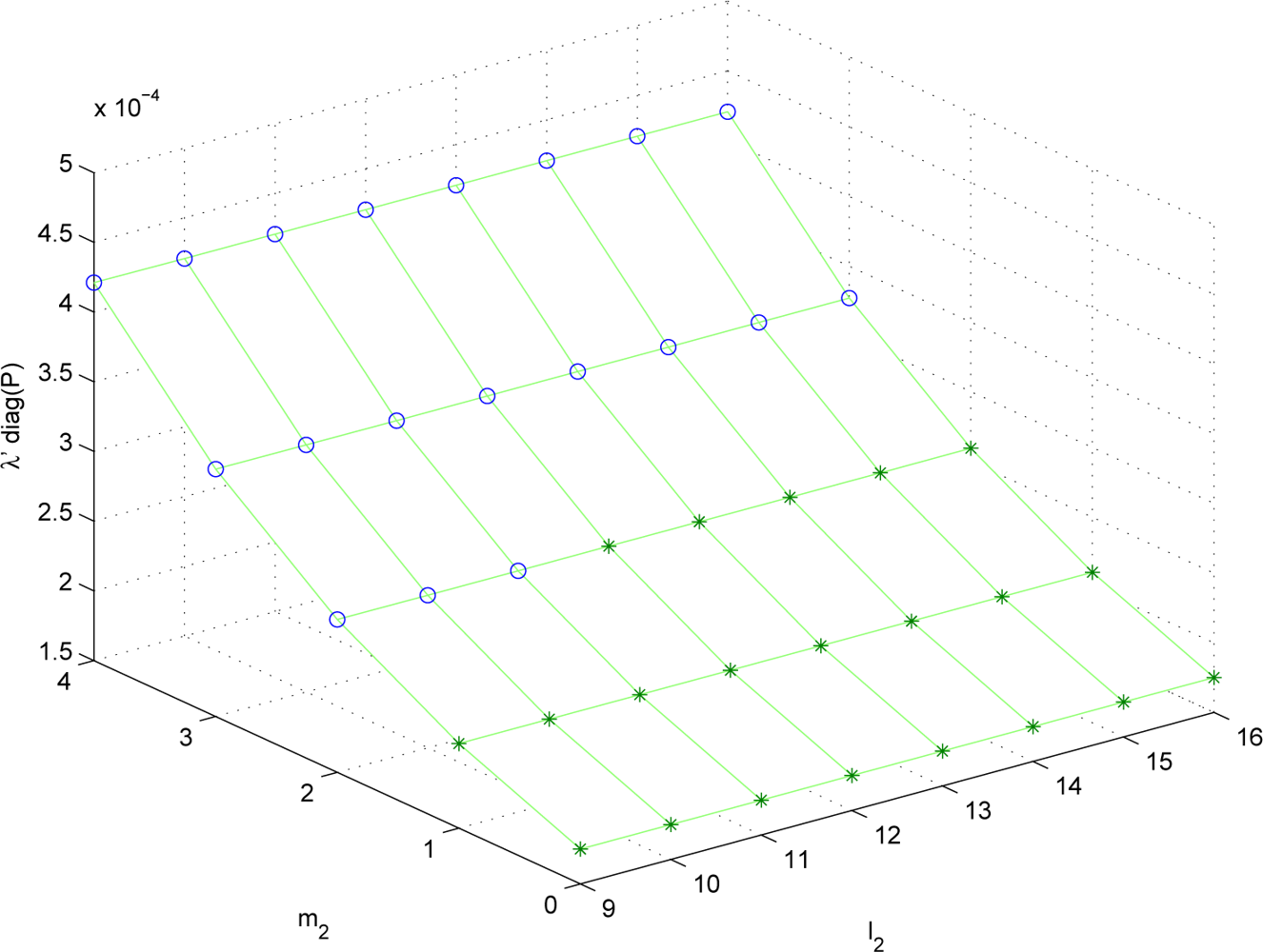
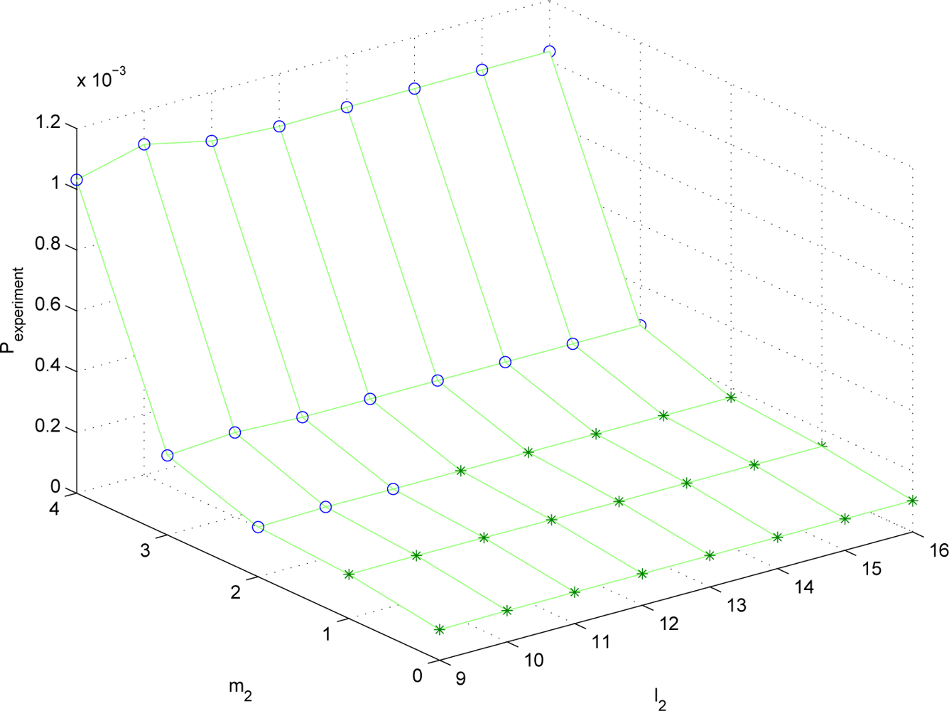
It can be seen that the optimal solution predicted by λP nearly coincides with the real optimal solution. To see how similar λP and P_experiment are, λP and P_experiment are plotted for different (m₁, l₁, m₂, l₂) combinations. Since the parameter space is four dimensional, it is not easy to visualize the result. Thus we fix (m₁, l₁) = (2, 9) and plot λP and P_experiment for (m₂, l₂) combinations in Figures 2 and 3. The data marked with “o” satisfies S ≤ S_max and the data marked with “*” does not satisfy S ≤ S_max.

It can be seen that the trend of λP is almost similar to that of P_experiment. Thus λP can be used to predict the estimation performance given the sampling periods and the quantization bit lengths.

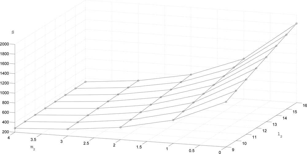
The transmission rate S is given in Figure 4. To see the trade-off between S and the estimation performance, S and λP are given for three (m₁, l₁, m₂, l₂) combinations in

Table 2. S and λP comparison

m1	l1	m2	l2	S	λP
0	16	0	16	3200	0.000080
2	12	2	12	600	0.000165
4	9	4	9	112.5	0.001282

. We can see that when S decreases (that is, if we transmit less data), λP tends to increase (that is, the estimation performance degrades).

Finally, to test the efficiency of the proposed algorithm, we applied the proposed algorithm to 100 random models, where A is randomly generated and the same C as in the previous simulation is used. In the brute force method, 479 combinations are tested as in the previous simulation since the same setting is used. In the proposed algorithm, the number of combinations tested is between 13 and 21. That is, the number of combinations tested in the worst case is 21. Thus we can see the convergence rate is relatively fast. To see the accuracy of the proposed algorithm, the following value is computed:

$$\text{Accuracy}\hspace{0.17em}=\hspace{0.17em}\lambda \frac{100\hspace{0.17em}\times \hspace{0.17em}(P_{\mathit{proposed}}\hspace{0.17em}-\hspace{0.17em}{P}_{\mathit{optimal}})}{P_{\mathit{optimal}}}$$

where P_optimal is computed using the brute force method. In the 100 trials, the worst case accuracy was 7.26% while the average value is 1.73%. Thus we believe the proposed method can find near optimal value while avoiding the large computation.

5. Conclusions

In this paper, attitude estimation over a network with a transmission rate constraint is considered. The transmission rate depends on the sampling periods and the quantization bit lengths. Basically the problem is trade-off between the estimation performance and the transmission rate, where the parameters are the sampling period and the quantization bit length.

First, how the sampling period and the quantization bit length affect the estimation performance is investigated. To do this, we introduced an augmented system and defined the estimation performance P. Secondly, the trade-off problem is formulated as an optimization problem and a suboptimal algorithm is provided. Through numerical examples, we showed that the defined estimation performance matches the real estimation performance in the sense that graphs of P and the real estimation performance are similar. We also showed the proposed algorithm could find a reasonably good solution.

While defining P, we made assumption (23), which makes the derivation of P easier but not essential. Removing that assumption and obtaining a general result is a future work. Also to test an algorithm using a real network is a future work.