1. Introduction
In recent years, a significant amount of work has been published in the field of colour segmentation for Human Computer Interfaces (
HCI). We would like to emphasize those related to the segmentation of the natural colour of skin. In this area, Phung
et al. [
1] proposed a skin segmentation method using a Bayesian classifier, obtaining satisfactory results for different colour spaces such as:
RGB, Hue Saturation Value (
HSV), Luminance blue-Chrominance red-Chrominance (
YCbCr) and Commission Internationale de l'Éclairage’s Luminosity a-channel b-channel (
CIE-Lab), even under adverse illumination conditions. Hsu
et al. [
2] suggested the detection of face skin considering a nonlinear subspace from the
YCbCr space to partially compensate the luminosity variations.
The robustness of the segmentation against luminosity changes is one of the most desirable features in colour segmentation systems. For this reason, much work on this topic has been focused on minimizing the effects of illumination changes by using colour spaces where the luminance or intensity component can be easily isolated, thus providing chromatic constancy. The actual trend in applications with important time-varying-illumination changes is to use dynamic colour models that can adapt themselves to compensate for variations of the scene illumination. In this area, an extensive overview of previous investigations in the skin colour segmentation field is presented by Sigal
et al. [
3].
The most frequently used colour spaces in these types of applications are
HSV [
3,
4] and normalized Red Green (
rg) [
5–
7]. The
HSV space, as well as the Hue Saturation Intensity (
HSI) and Hue Lightness Saturation (
HLS) spaces, are widely used in image processing because it is very intuitive for the human brain to interpret the information as it is represented. In some works, only the Hue (
H) and Intensity (
I) components are used in the clustering process [
8]. In other cases, a threshold value for the Saturation (
S) of each pixel based on its intensity is defined [
9]. This threshold is used before the clustering process to determine if
S should be replaced by
H or
I.
In general, all these segmentation proposals offer good results for objects with significant size in the scene or in cases where the main goal is object tracking, but not in the case of shape recognition. If the goal is to recognize the object shape, the system requirements are higher and very accurate segmentation techniques should be applied. Further difficulties may arise if the images have low quality and spatial resolution. Sign language recognition systems based on computer vision are a good example of these types of applications. In this case, the camera should capture all the upper parts of the speaker’s body, implying that the parts to segment (hands and face) constitute a small part of the captured scene. In this field, Habili
et al. [
10] performed a pixel-by-pixel classification of the skin colour with discriminant features of the
CbCr plane, using the Mahalanobis distance, but they needed a fusion of motion cues to obtain good results. Similar skin segmentation is achieved in the work done by Chai
et al. [
11], where post-segmentation stages were applied, such as morphological operations, in order to surpass the limitations of the segmentation. The
YCbCr space has been also used [
11]. This colour space is one of the most widely used in the segmentation process.
In this field, Ribiero and Gonzana [
12] presented hand segmentation in video sequences by means of the Gaussian Mixture Model (GMM) background subtraction algorithm, which is a well-known statistical model for density estimation due to its tractability and universal approximation capability. In this work, [
12], an adaptive Gaussian mixture in time is used to model each pixel distribution in
RGB space. In Huang and Liu’s work [
13], clustering of colour images using GMM technique in
HSV space is performed.
Less common colour spaces are also used in other works: both linear transformation spaces, like Luminance E-channel S-channel (
YES) [
14], and non-linear, spaces like the Uniform Chromaticity Scale (
UCS) spaces, such as Luminance u-channel v-channel (
L*u*v*) and its representation in cylindrical coordinates Intensity Hue Saturation (
IHS) [
15], Saturation Tint Value (
STV) [
16] which is a representation of
HSV space by the normalized
RGB components. Other spaces used are the Spherical Coordinate Transform (
SCT) [
17] and the geodesic chromaticity space
pq [
18].
We can also find works related to object/background segmentation with the objective of efficiently delimiting object edges. Some of these publications present the use of graph cuts in N-dimensional images to segment medical images from computed tomography (CT) scanners [
19,
20], and multilevel graph cuts to accelerate the segmentation and optimize memory use [
21]. From our point of view, the main disadvantage of these works is that they are not designed for real-time purposes.
The conclusion of these previous works is that important unresolved problems still exist in order to obtain efficient skin segmentation, especially if we take into account that many applications require real time processing, include complex scenes, are prone to important illumination changes, and the objects to segment (face, arms and hands) are small when compared to the captured scene.
Our contribution to the solution of this segmentation problem is to use an object/background pre-processing technique to enhance the contrast (in the HS plane) between the colours corresponding to the objects to segment and the background in each frame. This pre-processing consists of increasing the separation between the object and background classes in the HS plane to optimize the segmentation in that plane.
In our proposal, to increase the class separation, a colour vector of components Δ
R, Δ
G, Δ
B, is added to the
R,
G and
B images directly captured from the camera, modifying the value of each pixel (
n) to (
Rn+Δ
R,
Gn+Δ
G,
Bn+Δ
B). The objective of this paper is to present the process needed to obtain the values Δ
R, Δ
G and Δ
B that optimize the separation between the classes of interest once the image has been converted to the
HS plane. This optimization is carried out by means of an algorithm that maximises the Fisher Ratio. We have called the colour vector addition process “colour injection”. In our proposal, the colour injection process is achieved using the relationships between the
RGB,
YC1C2 [
8,
22,
23] and
HSI [
24–
26] colour spaces, and the properties of the
C1C2 plane.
Our system may be particularized to recognize sign language in real-time and special attention has been paid to the detection of the geometric form of the parts to segment, hands and face edges, in each frame. Our proposal has been thoroughly tested with very good results even with illumination variations, because it isolates the
I component. We always attempt to work outside the instability or achromatic zone of the
HS plane, due to the convenient redistribution in the
HS plane of the existing classes in the colour injected image (seen in [
15] for the
IHS space). In order to perform a comparative qualitative study between the segmentations of the original images and the colour injected images (proposal presented in this paper), a GMM clustering technique in the
HS classification domain is used. This technique has been used in a similar way for the
HSV space [
13]. In previous works, different formulations for the
HSI space can be found [
22,
24–
26]. We use the formulation proposed in [
26].
This paper has been organized as follows: Section 2 describes the basis of the proposed algorithm to increment the separation between classes. Section 3 presents the criteria considered when separating the classes. Section 4 describes the off-line initialization stage of the proposed algorithm. Section 5 details how to improve the separation between classes in the HS plane starting from their location in the C1C2 plane. Section 6 presents the algorithm that performs the optimal class separation. Section 7 describes how to obtain the colour vector for injection, and its effects in the captured images. Section 8 contains the experimental results, and Section 9 provides the conclusions and future work.
2. Overview of the Colour Injection Algorithm
The objective of this work is to improve the segmentation process using colour injection. In order to do that, a colour vector for injection is obtained for each captured image in the
RGB space. This colour vector is considered optimal, because it is calculated to maximize the separation between the classes to segment in the
HS plane (subspace where the segmentation is performed). For this reason, this colour vector will be called optimal colour vector in this paper and will be denoted by
ir. It is injected in the
RGB space and is calculated starting from significant samples (seeds) from the object to segment and from the part of the scene considered as background. The procedure to obtain the vector
ir, and the reason why it is optimal is explained in Sections 6 and 7. This optimal colour vector is given by:
where Δ
R, Δ
G and Δ
B are the increments of the colour components
R,
G and
B, respectively.
The optimal colour vector, ir, is injected in every frame of an image sequence in real-time applications to segment objects in colour images. Its efficiency has been especially tested in applications where a reduced contrast between the background colour and the colour of the object to segment exists, when there are illumination changes and the size of the object to segment is very small in comparison with the size of the captured scene.
An important property of the perceptual colour spaces (such as the
HSI space) is that they produce a maximum disconnection between the chrominance and luminance components. As a result, the luminance can be almost fully isolated, making the segmentation process more invariant to the changes in shades and illumination as in [
4]. For this reason, the analysis of the colour injection effects in the
HSI space is made only using the
H and
S chromatic components (
HS plane).
As the segmentation is performed using the HS components, we try to separate the representative vectors of the two classes (object and background) in angle (H component) and in magnitude (S component) using colour injection. However, special attention should be paid in this separation process to the variations of the dispersions (reliability) of both classes after the colour injection, because it has a very high incidence in the class separation process.
In short, if the original image is denoted by I, the optimal colour vector to add by
ir, and the coloured image resulting of the colour injection by I
i, is fulfilled:
The algorithm proposed in this work is formed by two clearly different stages: an off-line and an on-line stage. The off-line stage is an initialization phase whose objective is to determine the optimal number of existing classes in the initial frame, and, from that, to obtain the object (O class) and background (B class) classes needed to carry out their separation. The off-line stage is explained in detail in Section 4. The result of this stage is the set of significant pixels (seeds) in the RGB space that represent both classes, identified by: ORGB = {rO1, rO2… rON}, and BRGB = {rB1, rB2… rBM}, respectively, where rOr for r = 1, 2… N and rBq for q = 1, 2… M refer to the pixel vectors of the object and background classes, respectively.
The on-line stage is the novel contribution of this paper. Its objective is to determine the optimal colour vector to inject (
ir) for each frame in order to increase, optimally, the separation between classes O and B. The on-line process is executed before the segmentation process for each frame captured in real time.
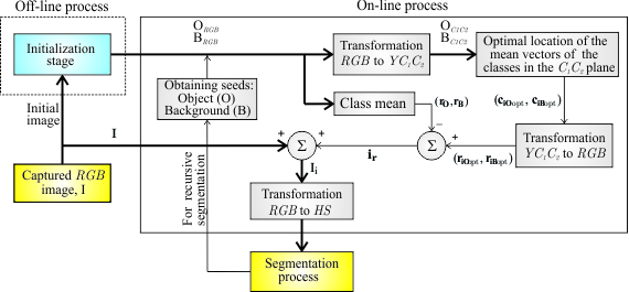
Figure 1 depicts the different phases of a segmentation process that uses the colour injection proposal of this paper.
The on-line process consists of the following stages:
For every ORGB and BRGB sample from the captured RGB image I, a transformation to the YC1C2 space is done. Considering the chromatic components after the transformation, the resulting classes will be referred to as OC1C2 = {cO1, cO2… cON} for the object class and as BC1C2 = {cB1, cB2… cBM} for the background, where the pixel vectors are denoted by “c”.
Using the properties of the C1C2 plane and the relationship between the HSI and YC1C2 colour spaces, the optimal location of the classes in the C1C2 space is obtained by finding the optimal location of their respective mean vectors. The optimal location is the one that maximizes the class separation in the HS plane (maximum distance between the class means and minimum class dispersions). These optimal mean vectors will be referred to as ciOopt and ciBopt. This phase is, undoubtedly, the most important of this work, and will be described in detail in subsequent sections.
From the mean vectors ciOopt and ciBopt, their corresponding ones in the RGB space, riOopt and riBopt, are calculated.
From the vectors
riOopt and
riBopt, and the mean vectors of the original classes (O
RGB, B
RGB) denoted by
rO and
rB, the optimal colour vector for injection is obtained. This optimal colour vector can be calculated from one of these expressions:
Once the optimal colour vector has been obtained, the new “injected” image Ii can be calculated applying (2).
Finally, the coloured image Ii is transformed from the RGB space to the HS plane, where the segmentation is done, because the colour injection has its effects in the HSI space: the increase in the separation between the classes only happens in the HSI space or HS plane (in the RGB space the colour injection only produces a translation of the classes, keeping the distance between them constant, independently of the colour injection).
The proposed method can be implemented easily and can be used in real-time applications. In the following sections, the process to obtain the optimal vector for injection is presented in detail. At the end of this paper, in order to facilitate its reading, we have included three appendices with aspects related to the relationships between the
RGB, the
HSI and
YC1C2 spaces (
Appendix A), statistical analysis of vectors in the
RGB space and its relationships with the components in the
HSI space (
Appendix B), as well as the invariants of the mean vectors in the
C1C2 plane (
Appendix C).
4. Initialization Stage (Off-Line Process)
The first step of the off-line process is the capture of a first frame (initial image). The seed pixels that represent the classes O and B are obtained from this image, by means of any clustering technique used to identify the existing classes of the image, such as K-Means [
30], GMM [
13],
etc. In this paper, the GMM technique is used (in the
HS domain) because it provides highly reliable classes, and, as a final result, it also provides the mean vectors, the covariance matrixes and the a priori probabilities of the classes. The clustering by means of GMM uses the EM algorithm (Expectation Maximization) to obtain the optimal location and dispersion of a predefined image class number (K), projected in the
HS plane. Therefore, a Gaussian model is assumed for each existing class, considering a uniform scene illumination. The GMM algorithm is applied several times, initializing it with different K values, in order to obtain the optimal number of existing classes in the image (K
opt). K
opt corresponds with the K that produces the smallest error in the log-probability function of the EM algorithm, indicating that it is the best fit between the K Gaussians and the existing classes.
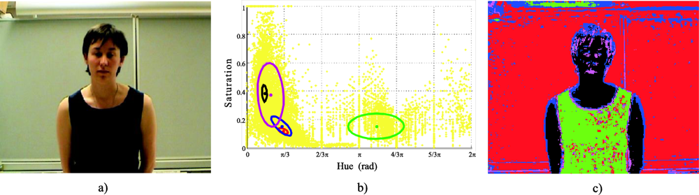
Figure 2b shows the K
opt Gaussians projected in the
HS plane, fitted to the existing classes in the initial image of the example in
Figure 2a. Finally,
Figure 2c depicts the original image segmentation as a function of the different existing classes (
Figure 2b).
Once the GMM algorithm has converged, the following step is to find out the localization of the object class (O) in the HS plane. This off-line process is carried out easily, because the approximate location of the object class (O) in the HS plane is known at the beginning of the off-line process, as a result of the colour calibration adjustments of the camera. This approximate geometric locus in the HS plane is given by the mean vector hinit. Taking that into account, the detection of the object class (O) is performed by simply selecting the class with the minimum Euclidean distance with hinit. We preferred the Euclidean distance over the Mahalanobis distance because the detection of the object class could be incorrect if hinit is close to a class with high dispersion, and this class is also close to the object class (O). The reason of this effect is the consideration of the class covariance in the Mahalanobis distance.
Once the object class is detected, the next step is to select the background class (B). The background is usually formed by several classes, identified by {B
1, B
2… B
Kopt−1}. Our objective is to select the B
k class that will be considered as representative of the background and that we will be identified simply by B. Among all the classes that form the background, we will select the B
k that:
being
PFRk; k = 1, 2… (K
opt − 1) the Fisher Ratio probabilities between the class O and each B
k, defined by
where
FRk is the Fisher Ratio described in Section 3, and
PBk; k = 1, 2… (K
opt − 1) the a priori probabilities of each B
k class to be the background class (B) of the image (given by the GMM algorithm).
Once the classes O and B have been identified, the seed pixels that represent both classes are obtained through an initial segmentation process of both the object class (O) and the background class (B). In this initial segmentation, the
pdf (probability density function) of both classes in the
HS plane are considered as unimodal bidimensional Gaussians, defined by the parameters obtained by the GMM clustering. This segmentation is carried out by selecting the pixels with higher probability to belong to the corresponding Gaussian. This stage of pixel selection is performed by truncating each class
pdf with a determined threshold. This threshold corresponds to a percentage of the maximum probability of the corresponding bidimensional
pdf, P
o, for the class O, and P
b for the class B. The values of {P
o, P
b} ∈ [1, 0], have been experimentally set to P
o = 0.45 and P
b = 0.6, using the Receiver Operating Characteristic (ROC) curves obtained from the different tests performed with real images. In this case a ROC curve was obtained by each class (O and B), using a set of real images, without and with colour injection. The thresholds P
o and P
b correspond with the nearest values to the elbows of the ROC curves. As the pixel selection is carried out in the
HS plane, it is necessary to truncate the
pdf in the Intensity axis, in order to obtain pixel sets that reliably represent the classes O and B in the
RGB space. The truncation of this unidimensional
pdf is necessary because the
H and
I components are independent (
Appendix A) (this is important when the clustering is carried out in the
HS plane) and this generates correspondence problems when the pixels in
RGB components are selected from its projections in the
HS plane. In this second
pdf truncation, the percentages selected of the maximum value of the
pdf intensity of each class are P
fo for O, and P
fb for B. These percentages have been set to P
fo = 0.4 and P
fb = 0.5.
Once the previous process is completed, a random sampling is carried out, selecting N samples for the class O and M for the class B, in order to reduce the working space dimension. This is the method to obtain the sets ORGB and BRGB mentioned in Section 2.
5. Separation of the Classes in the HS Plane from Their Location in the C1C2 Plane
This section details the most important relationships between the statistical mean and variance of the classes in the C1C2 and HS planes. Also, the effect of adding the same vector (colour injection) to two vectors in RGB space on the projections of these vectors in the C1C2 and HS planes is analyzed. This information is used to define an algorithm to easily calculate the optimal vector to inject in order to obtain the maximum separation between classes in the HS plane using translations in the plane C1C2.
5.1. Relationships between the HS and C1C2 Planes
Given two vectors in the
RGB space,
rO and
rB, the resulting projection vectors in the
C1C2 plane,
cO and
cB, and in the
HS plane,
hO and
hB, fulfil (see
Appendix A):
where
θc is the angle between
cO and
cB,
θh the angle between
hO and
hB;
dc is the distance vector between
cO and
cB,
dh is the distance vector between
hO and
hB; and
IO,
IB are the intensity means of both classes, object and background, respectively, corresponding to the
hO and
hB vectors.
f(
H) is a weighting function that depends on the
H component.
f(
H) ∈ [½, 1] (see
Appendix B).
It is important to note that, since the
C1C2 plane is linear, when adding a vector
ir (injected vector) to both
rO and
rB in the
RGB space, the distance vector
dc =
cO −
cB in the
C1C2 plane remains constant. These constant magnitude and orientation values (invariants of the
dc vector) are denoted by ‖
dc‖ and φ (see
Appendix C). Therefore, colour injections in the
C1C2 plane result in class translations, as in the
RGB space. This effect can be achieved with a translation vector
ic (corresponding to
ir) directly added in the
C1C2 plane.
Moreover, in the case of the C1C2 plane, (10) is verified (cosine law). Therefore, given that ‖dc‖ remains constant for the different values of ir, the values of θ, ‖cO‖ and ‖cB‖, will be modified as a function of the value of ir. In the case of the HS plane, it must be said that if ir is added to the vectors rO and rB (contrary to what happens in the C1C2 plane) the difference vector dh also varies. The reason is that, according to (11), dh depends on the value of IO and IB and on the f(H) weighting function. In any case (8) always holds.
In short, to calculate the value of the colour vector to be added in the
RBG space to obtain a particular separation between the classes in the
HS plane, the authors suggest using the relationships between the
h vector components in the
HS plane, and their corresponding
c vector components in the
C1C2 plane, given by (
Equation B.12) and (
Equation B.13) (see
Appendix B), and the relationship between pairs of vectors in these planes, given by (8, 9, 10 and 11).
Therefore, the proposed algorithm is based on the analysis of the behaviour of the vectors cO and cB in the C1C2 plane and the properties of its difference vector dc (‖dc‖ and φ are invariant). These invariants allow us to establish a mathematical relationship between the class mean vectors before and after the colour injection. Thus, for example, the separation angle (hue difference) between two vectors in the HS plane can be easily controlled with the separation angle of the same vectors (cO, cB) in the C1C2 plane, because both angles coincide (8).
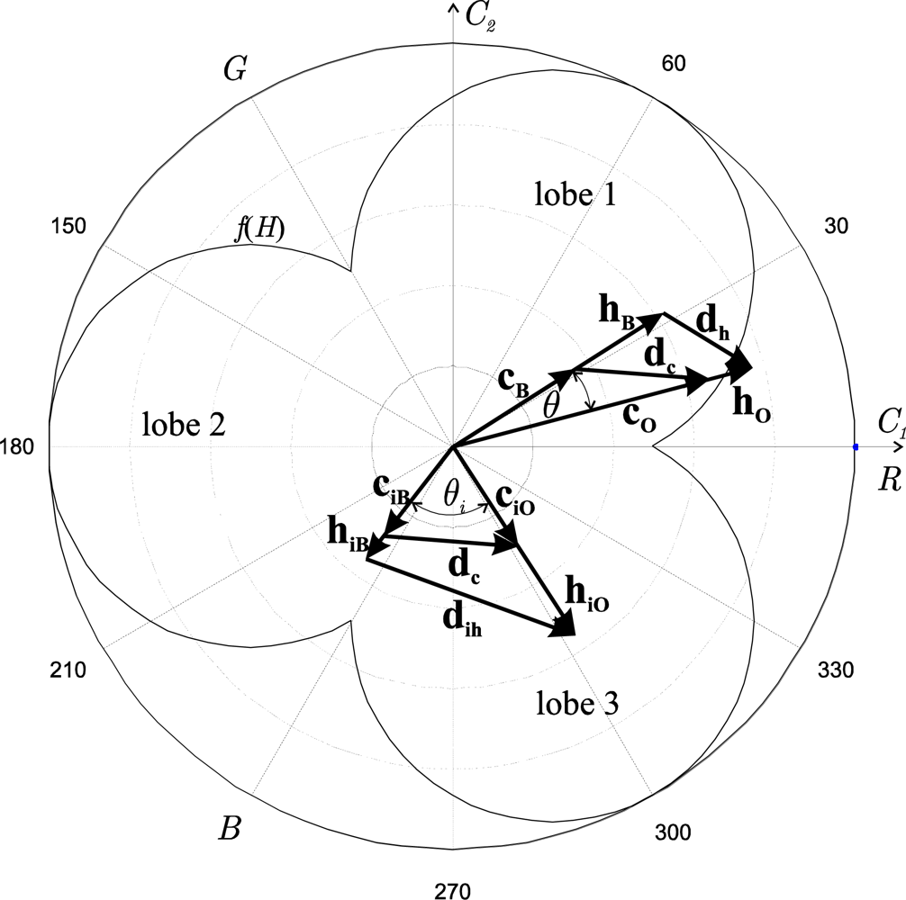
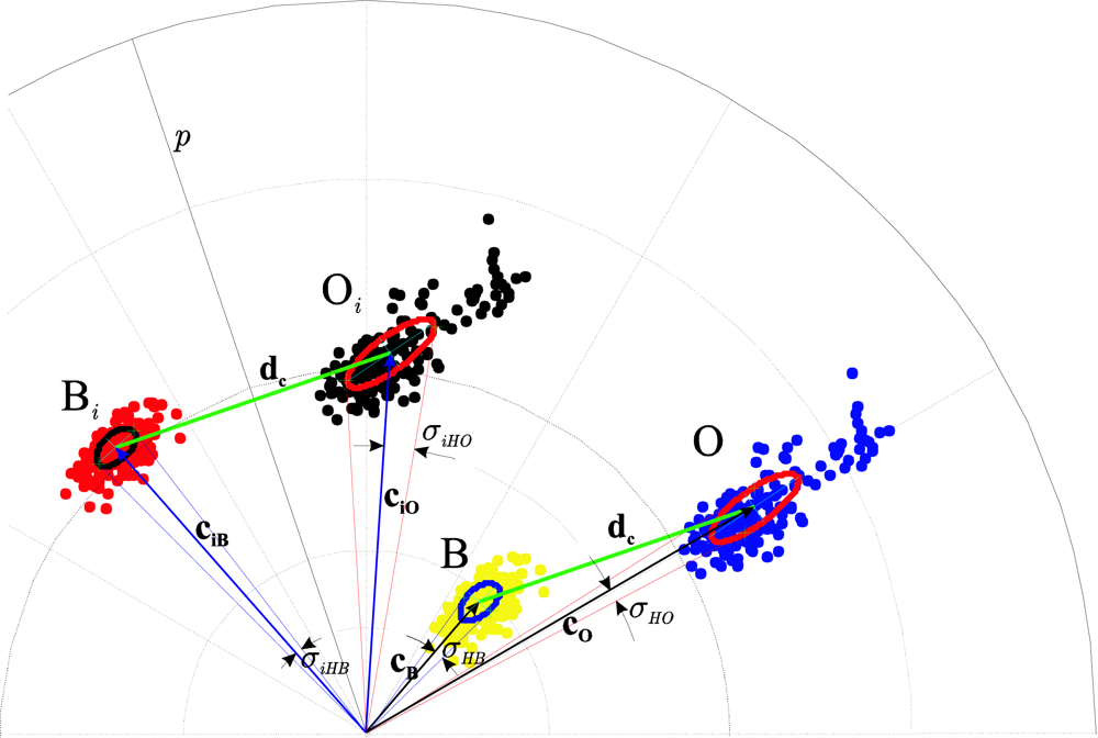
In
Figure 3, an example of the correspondence between the vectors
cO and
cB in the
C1C2 plane and the vectors
hO and
hB in the
HS plane is shown. The relationships after performing the colour injection (vectors
ciO,
ciB and
hiO,
hiB) are also shown, as well as the difference vector
dc before and after the colour injection, where the invariance in magnitude and angle can be observed. From now on, the “i” or “
i” subscript refers to “colour injection”.
Figure 3 depicts how the translation of the vector
dc has favoured the separation of the mean vectors of the classes in both components (
H and
S), because
θi >
θ, and (‖
hiO‖ − ‖
hiB‖) > (‖
hO‖ − ‖
hB‖). An increase in the separation between the vectors after the colour injection can be verified (
θI >
θ). However, the vector modules (saturation) decrease (‖
hiO‖ < ‖
hO‖, ‖
hiB‖ < ‖
hB‖), since there is an unavoidable compensation effect given by (10) (notice that for a fixed
I, ‖
h‖ =
const‖
c‖
f(
H)).
We could obtain a great number of class locations within the HS plane relocating dc with ic all over the C1C2 plane. The determination of the optimal location is not a trivial task. In order to obtain an optimal ic, it is possible to apply learning techniques, such as fuzzy systems and neural networks, that take as parameters some functions derived from FR’s (6) and the invariants of the vector dc.
In the following Section (5.2), an algorithm for the calculation of the optimal ir (corresponding to optimal ic), conditioned to ‖ciO‖ = ‖ciB‖, is explained.
5.2. Separation between the Hue Means (Angular Separation)
The separation between the hue means is given by the angular separation between the vectors
hiO and
hiB, which indicate the colour separation. Once the expression of the distance between
hiO and
hiB is obtained, ‖
dih‖ (see
Figure 3), an optimization process can be applied to it as a function of the
RGB components of
ir in order to obtain the optimal
ir that produces the maximum separation needed. The problem when calculating the optimal colour vector is that it is not possible to obtain its analytical expression, mainly due to the discontinuities in the function of ‖
dih‖ (11).
In order to solve the problem posed by the discontinuities of ‖dih‖ in the HS plane, the authors propose to use the C1C2 plane, where the distance function between the vectors ciO and ciB, (‖dc‖) (10) does not present discontinuities, and, as well, remains constant in magnitude and direction for different injections of colour vectors.
The interrelationship (due to the invariants of the vector dc and the relationships between the HS and C1C2 planes) between the angle (θi) that the vectors ciO and ciB form and their modules (10) should be taken into account to obtain the separation angle (hue difference) of two vectors in the HS plane. Therefore, the maximum separation angle between the vectors may imply (due to the compensation effect) a diminution of their modules, and, consequently, the saturation of both vectors. The saturation reduction of the vectors hiO and hiB implies that they become closer to the achromatic zone (the origin of the coordinates system), which means that the colours approximate to gray scale. The consequence of this phenomenon is the loss of discriminating power in the segmentation.
Therefore, the proposed algorithm has been parameterized as a function of the mentioned separation angle θi between the vectors ciO and ciB. In our case, the optimal angle θi is obtained from an observation function that measures the effectiveness of the class separation in different locations in the HS plane. This function will be described in paragraph f of Section 6.
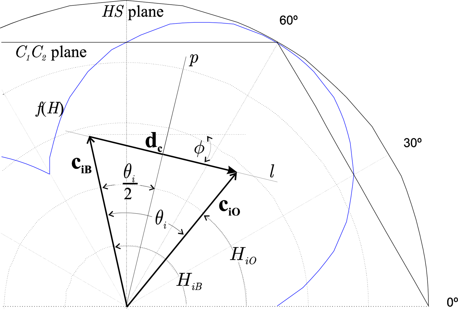
When the angle of separation
θi reaches a maximum,
θi coincides with the angle whose bisector is a straight line
p, which passes through the origin of coordinates and is perpendicular to the straight line,
l, whose director vector is
dc (
Figure 4).
Therefore, the vector for injection (
ir) that causes the maximum hue difference, causes the modules of both vectors
ciO and
ciB to become equal (‖
ciO‖ = ‖
ciB‖). It also causes the distance between the intersection point of the lines
p and
l and the extreme of each vector to be ‖
dc‖/2.
Figure 4 illustrates an example of the location of the vectors
cO and
cB after the injection of the colour vector (
ciO and
ciB) with those imposed restrictions.
The authors have given more importance to the angular (
H) separation, because increasing both
H and
S at the same time is not possible. The main reason is that
H has a discrimination power higher than
S. Besides, the
H component is totally uncorrelated to the
I component, which does not occur to the
S component (see
Appendix B). Parameterization only by
θi implies that we can only control the separation between the hue means. The starting point to obtain the distance between the saturation means is mainly the location of the vectors
ciO and
ciB with respect to the saturation weighting function in the
C1C2 plane. As can be observed, in this process there is no control on the
S component, so its contribution on the class separation will depend on the modification of the statistics of this component with the variation of
θi.
5.3. Separation between the Saturation Means (Saturation Difference)
In this section, an analysis of the behaviour of the separation between the saturation components of two vectors in the
HS plane is performed. Given two vectors, for example
hiO and
hiB, in the
HS plane, we analyze how the value of the saturation difference between both vectors
SO −
SB = ‖
hiO‖ − ‖
hiB‖ varies. In our case, as ‖
ciO‖ = ‖
ciB‖ =
Ci, then the intensities (
IO,
IB) corresponding to both vectors
hiO and
hiB, and the value of the saturation weighting function
f(
H) of each one, are the parameters with significant effect in the value of
SO −
SB. The reason is that, according to (
Equation B.11), the difference
SO −
SB will only have a non-zero value if
I and
f(
H) of both vectors are different (notice that the saturation varies inversely with the intensity, and directly with
f(
H)). As an example,
Figure 3 shows vectors
hiO and
hiB (overlapped to their respective vectors
ciO and
ciB), as well as the saturation weighting curve
f(
H). In the case of
Figure 3, the colour injection is done supposing
IO =
IB, therefore, the weighting function
f(
H) is the only responsible for the difference in the module of the vectors
hiO and
hiB, that is, of the separation between the saturation means of both classes. As previously indicated, in our proposal there is no control of the
SO −
SB value, but its behaviour as a function of the colour injections performed, parameterized by
θi, is known. According to this, it can be said that
SO −
SB is determined, as expressed in (12), by: (
a) the intensities of the vectors
hiO and
hiB (
IO,
IB), and (
b) the module and angle of
dc (the invariants) since these determine the location of the vectors
hiO and
hiB along the curve
f(
H) in the
HS plane. In the case of
Figure 3, where
hiO is located in the third lobe and
hiB in the second, it is fulfilled:
where:
5.4. Analysis of the Class Dispersion
In order to obtain the optimal vector for injection, ir, by means of the suitable election of θi, we should take into account not only the information given by the mean vectors cO and cB in the C1C2 plane, but also the dispersion of the distributions of both classes.
In this section we analyze the behaviour of the class dispersions in the HS plane, that is, how the hue and saturation dispersions are affected when the classes are translated in the C1C2 plane, as a result of the colour injection. A class separation measurement function will be defined to quantify the effectiveness of the colour injection. This analysis will be necessary to understand how the H and S dispersions are modified with the colour injection, in addition to the performance of the class separation measurement function.
5.4.1. Hue dispersion (Angular dispersion)
The hue dispersion is determined by the effects of the dispersion transformation when passing from the
C1C2 plane to the
HS plane. If
Ro is the (2 ×
N) matrix formed by the
N vectors of the O class:
cOr;
r = 1, 2…
N, before any translation, the parameters of the O class uncertainty ellipse,
i.e., the hue dispersion invariants, are obtained from the covariance matrix of
Ro, by:
where
ωO is the angle formed by the semi-major axis of the class uncertainty ellipse with respect to the horizontal axis (
C1), and
C1Ou and
C2Ou are the eigenvector components corresponding to the highest eigenvalue (
λOu) of the covariance matrix. The semi-major and semi-minor uncertainty ellipse axes,
uO and
lO respectively, which represent the maximum and minimum variance, are given by:
where
λOl is the minor eigenvalue of the covariance matrix. From these dispersion invariants, it is possible to obtain the model for the hue dispersion. Therefore, our interest is to obtain a correspondence between the hue dispersions in the
HS plane by means of the information offered by the angular dispersion in the
C1C2 plane. Knowing that the variation of the angular dispersion in the
C1C2 plane corresponds with the variation of the hue dispersion in the
HS plane, and since the
C1C2 plane is a Cartesian plane, the problem is posed in the polar coordinates, taking these two considerations into account:
As previously indicated, in the
C1C2 plane, the colour injections only produce translations of the classes and, therefore, variations of their mean vector modules (‖
ciO‖, ‖
ciB‖). This causes the modification of the angular dispersions of both classes, because they depend on
Ci = ‖
ciO‖ = ‖
ciB‖ (distance between the dispersion centre and the origin of the
C1C2 plane). These effects of the hue dispersion modification have been observed when performing translations of a class by adding Gaussian noise in the
RGB space [
22,
31]. In conclusion, the angular dispersion increases when the magnitude of its respective mean vector decreases due to the increment of the separation angle
θi, according to:
The geometric forms of the class distributions are not predetermined, but they can vary since they depend on the samples randomly taken from the object and the background. The colour injections produce class translations in the
C1C2 plane, implying that from the point of view of the
HS plane, the dispersion also depends on the geometric form of the classes. The reason is that, for different translations of a class, different orientations between the axis of maximum and minimum dispersion (represented by their uncertainty ellipse in a
C1C2 plane) with respect to the orientation of their mean vectors (
ciO or
ciB) are generated. Therefore, independently of the class mean vector module, a distance
da exists that contributes to the angular deviation. This distance
da depends only on the geometric form and orientation of the dispersion after each translation. Then,
da, in this case for the O class, will depend on the values of
ωO,
uO and
lO given by (13) and (14). This
da can be approximated by means of the distance between the centre of the uncertainty ellipse and the intersection point between two right lines: one is the tangent line to the ellipse which at the same time passes through the origin of plane, and the other line is perpendicular to the previous one and it crosses the centre of the ellipse. With
da and (15) the angular deviation can be approximated by:
As an example, in
Figure 5 we depict the object class (O) before a translation, for the addition of a vector
ic in this
C1C2 plane, or, for the injection of a vector
ir, directly to the classes in
RGB components. Over the object class, its respective uncertainty ellipse is shown.
In
Figure 5, we can observe that the semi-major axis of the ellipse is relatively aligned to the mean vector
cO of the class, causing the perception of the minimum angular dispersion of that class. It can also be observed that the module of this mean vector,
cO, before the injection is greater than the module of the vector after it has been injected,
ciO, which, therefore, is also perceived as a minor angular dispersion by this effect. We may conclude then, that the initial location of this class in the
HS plane represents a very favourable case, since the angular deviation before the colour injection is small.
Nevertheless, for the background class (B) before the colour injection, certain alignment between the mean vector
cB and the axis of greater dispersion of this class can also be observed, implying a reduced angular deviation. However, the problem is that the module of the vector
cB is reduced and, therefore, the angular deviation increases. In this case, it can be observed in
Figure 5 that after the colour injection, the angular dispersion of the class B
i is smaller, since the module
ciB is greater.
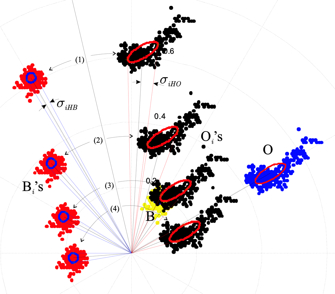
Figure 6 depicts another example, with the different class locations after four colour injections. The modifications of the angular deviations
σiHO and
σiHB of the object and background classes as a function of the orientation of their respective uncertainty ellipses and the modules of their respective mean vectors can be observed.
5.4.2. Saturation dispersion
The dispersion of the saturation component is not directly affected by the class translations (due to the colour injections) in the
C1C2 plane, if all the class vectors have the same intensity. The reason is that the saturation is a linear function of the
C1 and
C2 components. The expression of the saturation for lobe 1 of
f(
H) is (
Equation B.13) (see
Appendix B):
This characteristic of linearity in the C1C2 plane makes the deviation of the saturation (σS) constant, since the distance between vectors in the C1C2 plane remains constant, independent of the colour injection. Nevertheless, in the HS plane σS will be different for each lobe of f(H) but will stay constant within each lobe. Evidently, if the class vectors have different intensity, the dispersion of the saturation will not be constant for each location, not even within the lobes (there is a greater variation of σS when the dispersion of the intensity component is greater).
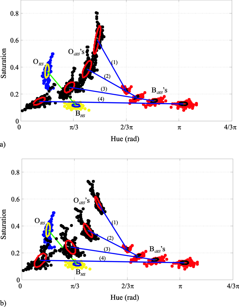
Figure 7 illustrates how the hue and saturation dispersions are modified for the four colour injections of
Figure 6.
In this case, the locations of both classes are projected in an
HS Cartesian plane. The magnitude of the
H and
S deviation can be appreciated by means of the projections of the corresponding uncertainty ellipses of both classes in the axes
H and
S. In
Figure 7a we can observe a diminution of the
H deviation and the increase of the
S deviation when the angle
θi between the classes decreases, because the modules of the mean vectors of both classes increase. It can also be observed how the
S deviation of the O
i class, is modified more than the deviation of B
i, because the
I dispersion of O
i is greater.
Figure 7b shows the same example as
Figure 7a, but with the intensities of the class vectors equal to its intensity mean,
i.e.,
IO1 =
IO2 = ... =
ION =
IO, and
IB1 =
IB2 = … =
IBM =
IB, implying that
σIO =
σIB = 0. Then, we can see how the
S deviation of O
i, remains constant for each colour injection.
However, our interest in this paragraph is to understand how the colour injections affect the saturation dispersion. This is the reason why in our algorithm the S deviations of both classes are obtained considering their original intensities.
6. Algorithm for the Optimal Location of the Mean Vectors of Both Classes in C1C2 Plane
This section presents the strategy used to obtain, in the
C1C2 plane, the mean vectors that maximize the separation between the classes in the
HS plane. This section constitutes the main stage in
Figure 1: “Optimal location of the mean vectors of the classes in the
C1C2 plane”. As shown in
Figure 1, for each captured image, an algorithm to obtain the optimal location in the
C1C2 plane of the mean vectors of both classes (object and background) is executed. From these optimal vectors,
ciOopt and
ciBopt, and once the transformation to the
RGB space is performed (
riOopt,
riBopt), the optimal vector to inject,
ir, is obtained using (3).
The proposal to obtain these optimal vectors,
ciOopt and
ciBopt, consists of different phases, and its general block diagram is depicted in
Figure 8.
As can be observed, the proposal includes an iterative algorithm to obtain a set of locations for the mean vectors of the classes (ciO and ciB) in the C1C2 plane. The location of each vector will be parameterized by the angle formed between both vectors, θi. Therefore, we try to obtain a set of θin (θi1, θi2…). Each of them will have associated a measurement index of separation between classes that we will identify by βHSn (βHS1, βHS2 …). From the function βHSn = f (θin), the value of θin that produces the maximum separation between classes is obtained, θin optimal: θopt.
The process begins obtaining the mean vectors of each class in
C1C2 plane. These mean vectors will be,
From the vectors
cO and
cB, its difference vector,
dc, is obtained. As previously indicated, the magnitude, ‖
dc‖, and angle,
φ, of the vector
dc are invariant against translations in the
C1C2 plane. Their values are given by
equation (19):
where
dC1 =
C1O −
C1B and
dC2 =
C2O −
C2B, such that (
C1O,
C2O) and (
C1B,
C2B) are the components of the vectors
cO and
cB, respectively.
The iterative process consists of the following six steps:
(a) Forced location of the mean vectors in the C1C2 plane
The original vectors
cO and
cB are relocated (forced) in the
C1C2 plane using the invariants (‖
dc‖,
φ), obtaining the new vectors (
cIo and
cIb). Each location of the vectors (
cIo and
cIb) should fulfil the following geometric restriction: the straight line that passes through the origin of the
C1C2 plane and is perpendicular to the vector
dc should intersect this last one in ‖
dc‖/2. As previously indicated, this implies that:
This θI is the parameter to vary in order to obtain the different locations of the vectors CIO and CIB, and, therefore, of the locations of the classes in the C1C2 plane.
The Cartesian components of these vectors (
Figure 4), particularized for the vector
CIO, are given by:
where
hIO is the angle of the vector that can be expressed by:
Similar expressions can be obtained for CIB.
The iterative algorithm is initialized with an θi equal to θ (θ is the angle formed by the vectors cO and cB). In each iteration (j) of the algorithm, the value of θi is increased: θi(j) = θi(j − 1) + Δθ.
We should also take into account that θi represents the hue distance between the mean vectors (HIO and HIB) of the classes in the HS plane. This indicates that a direct relationship exists between the class translations in the C1C2 plane and the hue separation distance between the class means in the HS plane.
(b) Verification of the validity for the locations of the CIO and CIB vectors
For each increase of θi, the validity of the locations of the vectors CIO and CIB is verified. In case they are valid, the value of θi is included in the set θin. The validity of CIO and CIB (validity of θi) is tested by checking if the components of the corresponding vectors in RGB space (RIO, RIB) fulfil the limitations imposed by this space, i.e., the values are in the range [0, 1], because they are normalized with respect to 255.
(c) Calculation of the class translation vector in the C1C2 plane
The translation vector
ic is obtained for each value of
θin. This vector
ic is responsible for the class translations from its original position to the forced location defined by
θin. The translation vector
ic in the
C1C2 plane corresponds to the vector to inject
ir in the
RGB space. This translation vector can be calculated from any of the following expressions:
(d) Translation of the classes in the C1C2 plane
The class translations in the
C1C2 plane are performed with the value of
ic that has been calculated. Therefore, each vector
c belonging to the object and background classes are increased by
ic:
(e) Class transformation from the C1C2 plane to the HS
(f) Observation function: calculation of the class separation measurement index (βHSn) in the HS plane
As the class separation observation function, a normalized measurement index has been defined (
βHS) from the
FR described in (5). It has been normalized to obtain
βHSn = 1 when the class separation is maximum. To obtain the
βHSn corresponding with each
θin, we consider the mean and the dispersion of
H and
S of the classes, according to (6). Therefore, two class separation measurement indexes as a function of
θin have been defined, one for each component:
The final class separation measurement index is given by:
where
kh is a weighting factor between
βHn and
βSn. The value of
kh ∈ [0, 1] is chosen depending on the prominence we want to give
H or
S in the segmentation process. Taking into account that
H has a greater discriminating power than
S,
kh > ½ should be fixed.
This iterative process is repeated until the first non valid value of θin is generated, and the pairs (βHSn, θin) are registered to obtain the function βHSn = f(θin) afterwards.
Once the set of pairs (
βHSn,
θin) is obtained, the
θin that produces the maximum class separation measurement index is selected. A cubic interpolation is performed around that local maximum to obtain the maximum of the interpolation index,
βHSmax, and its associated angle,
θopt. Finally, with this
θopt, the
ciOopt and
ciBopt vectors are obtained using
(20),
(21) and
(22).
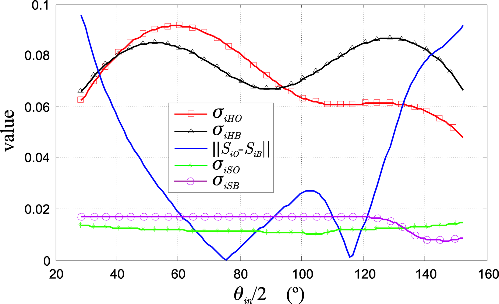
As an example,
Figure 9 shows the variation curves, as a function of
θin/2, of the statistical data: deviations of hue (
σiHO and
σiHB), deviation of saturation (
σiSO and
σiSB), and difference between the saturation means ‖
SiO −
SiB‖ needed to obtain the different class separation measurement indexes (25).
7. Calculation of the Optimal Colour Vector to Add and the Effects that it Produces on the Images
The calculation of the optimal colour vector to add, ir, is the goal of our proposal, because this vector changes the colours of the captured image in a suitable manner, so that the classes separate and, therefore, the object class can be more easily segmented.
Figure 10 shows the values of
βHn,
βSn and
βHSn obtained from the values of the statistical data depicted in
Figure 9. The values of (
θopt,
βHSmax) obtained by interpolation are also shown.
As depicted in the block diagram of
Figure 1, once the vectors
ciOopt and
ciBopt, that represent the optimal location of the classes in the
HS plane, are obtained, the vectors
riOopt and
riBopt can be calculated. Thus, for instance, for the object class, O: if
C1Oopt and
C2Oopt are the
C1 and
C2 components of the vector
ciOopt respectively, the vector
riOopt in
RGB space is obtained by:
where
Q is the transformation matrix (
Equation A.2) and
YiO is the intensity mean of the object class translated in the
C1C2 plane. The
ir vector is obtained with this
riOopt applying (3). Considering that the colour injection can be made without modifying the mean intensity of the class after the injection of
ir,
YiO =
IO holds. Although it is possible to modify the saturation mean varying the intensity mean, in this case, we want the saturation mean to be only affected by the
f(
H) value and the Chroma component (
C). Therefore, the vector to inject,
ir, should have zero mean (E{
ir} = 0). The fact that E{
ir} = 0 implies that the intensity mean of the original image (I) and the injected one (I
i) are equal.
The effect of injecting the vector
ir to the original image in the new image, I
i, is a greater concentration of the pixel colours around the mean colour of each one of the two classes. That is, the colour injection contributes to the histogram equalization of the captured image in the
HS plane. This equalization has a concentration effect on each class, and, therefore, the injection of
ir contributes to approaching the class distributions to a Gaussian shape. As an example,
Figure 11 shows the 2D histograms of image I (
Figure 11a) and of the coloured image resulting from the colour injection I
i, (
Figure 11b), for a particular case (
Figure 12 images).
In these
figures (11a and
11b), the equalization of the histogram produced by the effect of the colour injection can be clearly observed. The segmentation of both images is shown in
Figure 12c and
12d respectively. In this example, K
opt = 4, the O class corresponds with the jacket and the B class with the wall.
The effect of the class separation between O and B classes can also be directly seen, analyzing the class locations before and after the colour injection in their histograms.
Figure 13 shows the histograms corresponding to the sets O
HS and B
HS in (a), and the sets O
iHS and B
iHS in (b). A remarkable increase in the hue component separation can be observed in the histograms of
Figure 13b due to the colour injection.
The rest of the image classes different from B, B
x ≠ B;
x = 1, 2 … K
opt − 2, are also affected by the effects of the colour injection. In this sense, as the class selected as B is the closest to the class O that also has a high probability to be the image background (fulfils
equation (7)), when the separation between the classes O and B increases, the classes B
x also increase their separation with the class O. However, the colour injection decreases the separation between the class O and those classes B
x (B′
x; x = 1, 2 …) that are closer than B to the class O but that were not selected as class B because they had a lower a priori probability. The consequence is that these classes (B′
x) can be considered as class O, producing false positives in the object pixel classification.
Another effect of the colour injection is the automatic compensation of the illumination changes. That is, due to the equalization and the separation of the classes O and B in the injected image, there is a minimization of the problems produced by the illumination changes. The reason is that the main colour component affected by the illumination changes is S, and, as previously explained, our algorithm gives more importance to the separation of the most discriminant component, H. Then, both classes, O and B, always keep a certain separation, independently of the parameter variation of both distributions, and mainly when the mean and variance of the S component vary due to changes in the luminous intensity.
Next, in
Figure 14, three histograms are presented, for the original and the injected image. All of them have been obtained with the different mean luminous intensity of the image (
Im = E{I} = E{I
i}): (
Im1 = 0.70,
Im2 = 0.45 and
Im3 = 0.21). The illumination compensation effects mentioned above can be observed in this figure.
8. Experimental Results
A bank of real images from different scenes has been used in a first phase of the practical tests, in order to evaluate the effectiveness of the proposed method. Here, a Gaussian classifier has been used as a segmentation technique, supposing a unimodal Gaussian model for the respective object and background class-conditional
pdfs,
i.e.,
p(
hi|O
i) and
p(
hi|B
i). Thus,
p(
hi|O
i) =
g(
hi;
hiO,
ΣiO) is given by:
where
hi represents each pixel of the image I
i, and
ΣiO is the covariance matrix of the injected object class in the
HS plane. The segmentation is performed by thresholding the
pdf (28) with a
Th value. This threshold is obtained knowing that we want to segment the class O
i taking the background class B
i as reference, so,
Th corresponds to the value of
pdf (28) when:
. Therefore,
Th is given by:
The problems derived from the cyclical nature of the hue in the segmentations have been solved via software, using the convention introduced by Zhang and Wang [
8].
In the evaluation, the same number of samples (seeds) for the object class (O) and the background (B) has been taken,
M =
N, in order to ensure that the difference between their statistical data is for intrinsic reasons, and not for differences in the sample space dimension. In the tests, the following data have been used: samples number:
M =
N = 50. Other tests with a higher number of seeds (
M =
N = 100, 200, 400, 800 and 1,600) have also been carried out, providing similar qualitative results in all of them, but with an increase in the iterative process computational cost. The increase of
θ used in the algorithm shown in
Figure 8:
Δθ = 5°, interpolation interval
ΔΘ = ±3
Δθ and the weighting factor
kh in (26) has been experimentally selected for each experiment, always fulfilling
kh ∈ [0.75, 0.97]. In this stage, the experimental results have been quantified by means of the
FR defined in (5).
Table 1 shows the values of
FR for 14 cases of the bank of images used in the tests.
Fourteen examples of segmentation can be seen in
Figure 15 (figures a, b, c, d, e, f, g, h, i, j, k, l, m and n) that correspond with the 14 cases of
FR calculated in
Table 1. Four images are shown in each column (from up to down): the upper image is the original one (I), the second one is the coloured image (I
i), the third one, the results of the segmentation of the original image (I segmentation), and the lower one, the results of the segmentation of the injected image (I
i segmentation). The segmented images show the object pixels in green colour. For the figures between
Figure 15a and
Figure 15m, the object class (O) is the skin, and for
Figure 15n, the object class is a jacket.
As can be observed, our proposal to inject a colour vector allows the attainment of remarkable improvements in the segmentation process, even with a segmentation technique as studied and effective as the Gaussian classifier.
As a second phase of the experimental tests, and in order to quantify the improvement in the segmentation of the injected image with respect to the original image, an analysis, pixel by pixel, has been made, comparing with the manually segmented reference images for the 14 cases. The data generated in this analysis, without noise added, are shown in
Table 2. The performance of the segmentation has been measured taking into account the classification Correct Detection Rate (
CDR) and False Detection Rate (
FDR) and the total Classification Rate (
CR).
CDR is the percentage of object pixels correctly classified,
FDR is the percentage of background pixels incorrectly classified and
CR is the total percentage of correctly classified pixels.
Table 2 also shows the number (K) of Gaussians used by the GMM algorithm, the
FR obtained by the statistics given by GMM for both classes, as well as the
kh used for each image.
Table 3 shows the results of the comparison of the same images, but contaminated by additive zero-mean Gaussian noise. As can be seen, results obtained with the colour injection technique for both tests are better than those obtained using only a Gaussian classification.
As a third phase of the tests, an example of image sequence segmentation is presented. In this case, each frame illumination has been modified before the segmentation process, in order to verify the advantage of our proposal against illumination changes. The illumination is applied to each frame in a uniform way. A zero-mean Gaussian noise with standard deviation np = 0.15IO was also added to the pixels of the images. Moreover, a sinusoidal time variation in the luminous intensity has been set up.
With this example, we try to show the improvements in the segmentation phase when the colour injection preprocessing step proposed in this paper is used before the segmentation. In this example, the GMM technique is used as an on-line segmentation technique (the same used in the off-line process). The original image I is identified by Ik for each captured frame in time kT (k = 1, 2... and T = time between consecutive images), and its corresponding image after the colour injection,
, are segmented using the optimal class number obtained as a result of the off-line stage. In this case Kopt = 5.
For the images I
k and
, the GMM segmentation process is applied recursively using the a priori probabilities, means and variances obtained in the images I
k−1 and
, respectively. For the segmentation of the image
, the next steps are also added: (
a) we obtain the pixels (seeds) in the
RGB space of the object and background of the image
, (
b) the vector
ir is subtracted from them, (
c) they are transformed to the
HSI space, (
d) the truncation process described in Section 4 is applied, and, finally, (
e) the sets
and
are obtained. These steps (
a,
b,
c,
d and
e) represent the block: “Obtaining seeds: Object (O) and Background (B)”, for recursive segmentation in the block-diagram of the
Figure 1.
In image sequence segmentation, as this example, the iterative process (seen in Section 6) has been slightly modified in order to reduce the processing time and to increase the stability of the colour injection in time. The first modification, is to use
(
θopt of the previous frame) as a starting point to obtain
, thus reducing the search interval to:
. In the example of
Figure 16, we have fixed experimentally
θf = 12°,
Δθ = 1° and
kh = 0.91. The second modification in the iterative process is that the optimal colour vector to inject
is obtained recursively, using for the calculation of
the following expression:
, where
kt ∈ [1, 0] is the constant fixed to obtain a proper smoothing of the evolution of the different parameters involved in the colour injection.
kt has been fixed experimentally to 0.1.
The GMM technique is used in these tests, mainly to obtain a better adjustment of the Kopt Gaussians in each frame, and, therefore, to obtain the maximum quality in the object segmentation. Then, a reliable comparison of the segmentation quality between the segmentation of the images I and Ii in the time can be carried out, and the compensation effects in the segmentation against illumination changes, applying the colour injection or not, can be verified. However, as it is known, this technique may have a relatively high computational cost due to the convergence iterations of the EM algorithm, so, its use in video segmentation is sometimes limited. For the consecutive segmentation of an image sequence in real time, our proposal in this work is to track recursively the parameters that define each Gaussian: O and B, using the optimal estimation provided by the Kalman filter, tracking technique widely studied in the image processing field.
Figure 16 shows the results of the segmentation of the images I
k and
of the example sequence, for the frames captured in
k = 21, 42, 63, 84, 105, 126, 147, 168, 189 and 210. The respective mean intensities of these frames are:
,
,
,
,
,
,
,
,
and
.
However, if the variation of the parameters of the different classes of the scene in the image sequence is very small, that is, when the scene is relatively uniform in the time with small illumination changes, the colour injection can be carried out applying the same colour vector ir to each frame in the time kT, with no need to recalculate it. This is possible due to the illumination compensation effect previously mentioned in Section 7. In this sense, the segmentation can be carried out keeping the parameters of both Gaussians as fixed values in all the sequence. Then, the computational cost is noticeably reduced.
Figure 17 depicts the results of the segmentation of the images I
k and
corresponding to the instants:
k = 50, 100, 150, 200, 250 and 300 of the previous example image sequence, but, this time, without recalculating the colour vector
ir and with fixed parameters for both Gaussians. The objective of this example is to appreciate the improvement in the segmentation of the sequence of colour injected images, although the same colour vector
ir is used in the injection.
In
Figure 17, the upper row depicts the I
k images, the central row shows the results of the segmentation without colour injection (I
k segmentation), and the lower one contains the results of the segmentations after the colour injection proposed in this work (
segmentation). The segmented images show the object pixels in green colour. The segmentation process used in this phase has been used in the first stage of the experimental tests.
As a reference, the average execution time (Tp) in Matlab of the on-line process for different M = N values is approximately: Tp = 74.9 ms. for N = 50, Tp = 80.0 ms. for N = 100, Tp = 85.4 ms. for N = 200, Tp = 95.9 ms. for N = 400, Tp = 117.3 ms. for N = 800 and Tp = 160.4 ms. for N = 1,600. The tests have been made with the following configuration: θf = 12° in the recursive process, 10% of pixels segmented in the previous frame are used to obtain the
and
sets, and the image size is 346 × 421 pixels. The image size affects the execution time of the injection of ir to the original image, and the conversion of the injected image to the HS plane for its posterior segmentation. The tests have been carried out in a PC with a processor Intel Core 2 Duo with a 2.4 GHz frequency.
Finally, we show some results of the real-time segmentation of images captured in a scene with significative illumination changes. These results highlight again the advantages of using the colour injection proposal presented in this paper.
Figure 18 depicts the comparative results in two columns: the left column (a) shows the segmented images without the colour injection, and in the right one (b) the images segmented after applying the colour injection.
The segmentation has been performed by thresholding the
pdf of the skin class seen in (28), once all the classes have been obtained with the GMM algorithm. In this case, K = 10 predefined classes were used. In order to demonstrate the robustness to illumination changes, an incandescent light bulb has been used (that produces a hue change in the whole image that tends to yellow) to really change the illumination of the scenes. The different luminous Intensity levels have been quantified with the mean intensity of the image normalized between [0, 1]. The corresponding Intensity levels for the five images of each column of
Figure 18, starting from the image above, are: I
1 = 0.351, I
2 = 0.390, I
3 = 0.521, I
4 = 0.565, I
5 = 0.610.
In the performance of this last practical test, a PC with an Intel Quad Core Q6600 @ 2.4 GHz processor and 2 GB SDRAM @ 633 MHz memory has been used. Although it is a last generation PC with four processing cores (CPUs), our application has only used a single CPU. A Fire-Wire video camera with a 1/2” CCD sensor with a 640 × 480 spatial resolution and an image capture rate of 30 fps (RGB without compression) was used. The optic used is a C-Mount of 3/4” with a focal length of f = 12 mm. The different algorithms of our proposal (GMM, colour injection and segmentation) have been developed in C, under Linux OpenSuSE10.3 (×86_64) operating system. With this configuration, the average processing time of the on-line process (Tp) is approximately 2 ms for N = 50.


