Electromagnetic Imaging Methods for Nondestructive Evaluation Applications

Abstract
: Electromagnetic nondestructive tests are important and widely used within the field of nondestructive evaluation (NDE). The recent advances in sensing technology, hardware and software development dedicated to imaging and image processing, and material sciences have greatly expanded the application fields, sophisticated the systems design and made the potential of electromagnetic NDE imaging seemingly unlimited. This review provides a comprehensive summary of research works on electromagnetic imaging methods for NDE applications, followed by the summary and discussions on future directions.1. Introduction
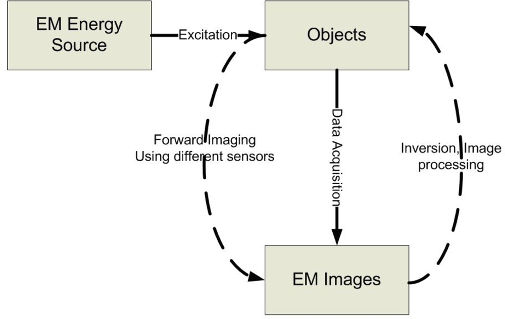
The development of imaging techniques for investigating physically inaccessible objects has been a topic of research for many years and have found widespread applications in the field of nondestructive evaluation (NDE) [1]. All electromagnetic (EM) methods in nondestructive evaluation involve Maxwell’s equations and cover a broad range of the electromagnetic spectrum, from static or direct current (DC), such as magnetic particle method, to high frequencies, e.g., X-ray and gamma-ray methods. Imaging, simply speaking, is the formation of images. Imaging science is concerned with the formation, collection, duplication, analysis, modification, and visualization of images. Electromagnetic NDE imaging is essential for detecting anomalies or defects in both conducting and dielectric materials by generating two-dimensional (2D) or three-dimensional (3D) image data based on the electromagnetic principles. A generic EM NDE imaging system can be simply represented as shown in Figure 1. For the forward imaging approaches, the excitation transducers usually couple the EM energy into the test objects, while the receiving sensors measure the response of energy/material interaction. Depends on different energy types and/or levels, various EM sensors/transducers can be used for a broad range of applications, e.g., eddy current imaging, microwave imaging, terahertz imaging, etc. After acquiring and storing the EM images, those data are passed through the inversion techniques block, which involves the object reconstruction, pattern recognition, etc. [2].
The usable electromagnetic frequencies for NDE purposes cover almost the entire EM spectrum, from DC to gamma radiation at the short wavelength end. However, this review article covers the imaging methods according to the different excitation EM frequencies only up to terahertz (THz). The reasons are two-fold: first, the optical NDE imaging with frequencies as low as in infrared range has been recently reviewed by another group [3]; second, the paper is intended to summarize and discuss the image modalities from the fields and waves perspective. As a result, the X-ray and gamma-ray NDE imaging techniques are not included here. Meanwhile, for non-EM methods, a heavily cited review article authored by Achenbach on quantitative NDE but focusing on acoustic imaging and applications was published in 2000 [4], which the readers can refer to for a complete understanding of NDE imaging methods.
2. Techniques Based on Different Electromagnetic Frequencies
The EM NDE imaging techniques covered in this review article include: direct current (DC) or static imaging methods, such as magnetic flux leakage imaging and impedance tomography imaging, to low frequency eddy current (EC) imaging that includes conventional EC imaging, EC sensor arrays, EC tomography and recently developed high resolution EC-based microscopy. Within the high frequency bands, microwave imaging, millimeter wave imaging and THz imaging are discussed. Some emerging methods like hybrid EM imaging, super-conducting quantum interference device (SQUID) imaging are also briefly summarized at the end of the paper. Overall, this paper is organized based on the different frequencies from longer wavelength end to shorter wavelength end those are applied in the EM imaging. Inverse problems in imaging such as image reconstruction, image characterization and analysis are also included in each section as key components of EM NDE imaging.
2.1. Static Electromagnetic Methods
In 1988 and 1990, Jiles at Center for Nondestructive Evaluation (CNDE), Iowa State University published two comprehensive and pioneering reviews about a variety of magnetic methods for NDE on ferromagnetic materials [5,6]. Magnetic particle inspection, magnetic flux leakage, leakage field calculations and eddy current inspection, including the remote field electromagnetic inspection method have been briefly discussed in his papers and he foresaw that with the upsurge of interest in that field, there must certainly be new magnetic methods awaiting development in the near future. In the past two decades, his statement has been validated as numerous electromagnetic imaging methods were developed while the ongoing research in this field still offers wide scope for future development and growth. In comparison with ultrasound, the instrumentation required in EM imaging is becoming far complicated than it used to be. However, the unique advantages that EM imaging has made this field promising, which is also the main driving force for the authors to review the current EM NDE imaging that are up to date through this article.
2.1.1. Magnetic Flux Leakage Method
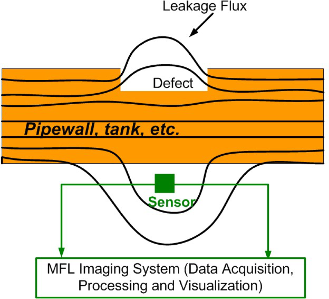
Magnetic flux leakage(MFL) method is one important and widely used techniques in static eletromagnetic imaging methods. It is used for nondestructive evaluation of ferromagnetic objects and generates grey scale images that are representative of the integrity of those objects. Defective areas typically appear as bright regions in the image. The schematic of an MFL imaging system can be found in Figure 2. It clearly shows effects of induction on magnetic lines at discontinuity: surface leakage flux occurs at high magnetization level and with defects present, then gets picked up by the MFL sensors before passing to the imaging system for processing.
Since early 1990s, Udpa’s Materials Assessment group at Iowa State University (now Nondestructive Evaluation Laboratory at Michigan State University) were one of the pioneering groups in the US conducting MFL inspection and imaging research [7–10].
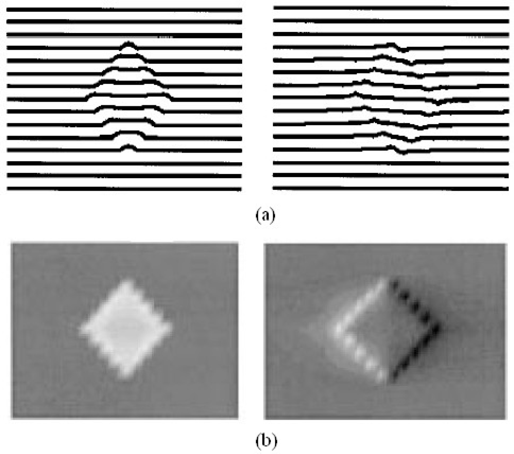
Their work mainly focus on defect characterization using MFL imaging data while the effect of variations in the test parameters associated with the experiment presenting. Mandayam and Udpa developed several novel but general techniques for deriving selective image invariants and performing invariance transformations to compensate for such variations. For example, wavelet basis functions can be used and typical magnetic flux leakage images obtained from finite element (FE) simulation of the pipeline inspection process are presented in their paper [7].
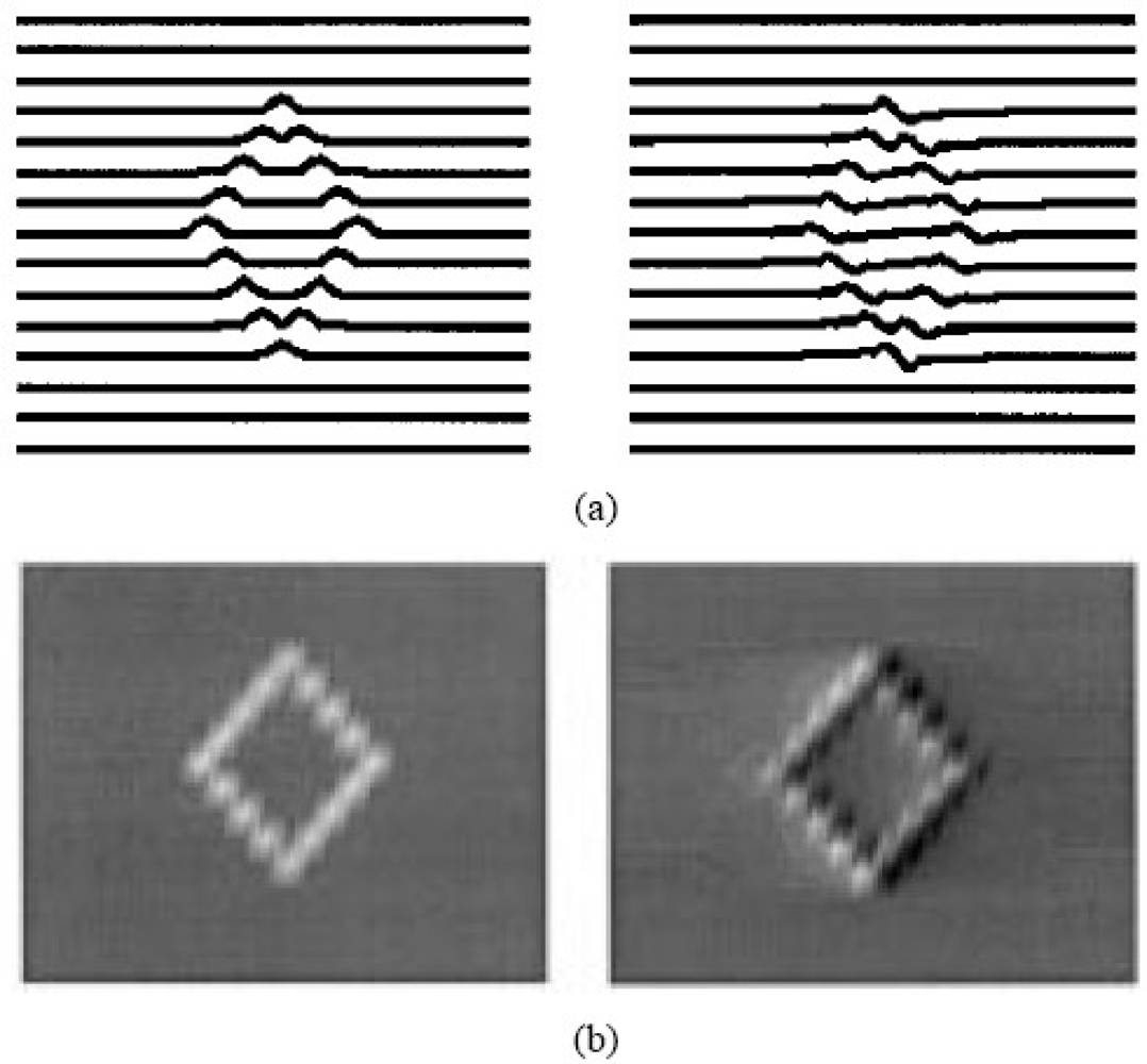
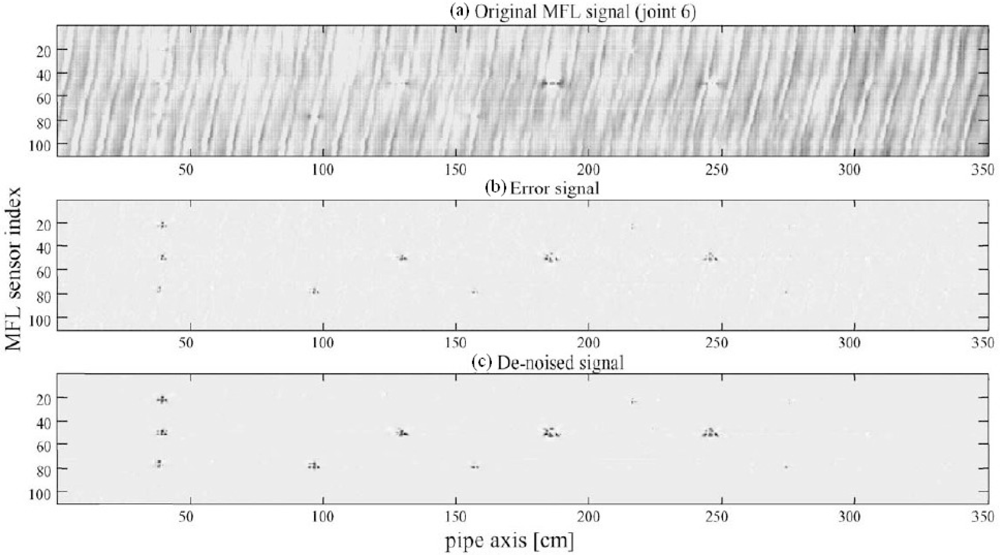
In 2002, Afzal and Udpa introduced a new technique that employs wavelet based de-noising and adaptive filtering for detecting signals in MFL images, which were obtained from seamless pipes [8]. The proposed algorithm is computationally efficient and data independent. Field test imaging results before and after the seamless pipe noise (SPN) removal are shown in Figure 3. The stripe pattern can easily bury the useful information and significant improvement has been demonstrated according to the original MFL image and de-noised images comparison.
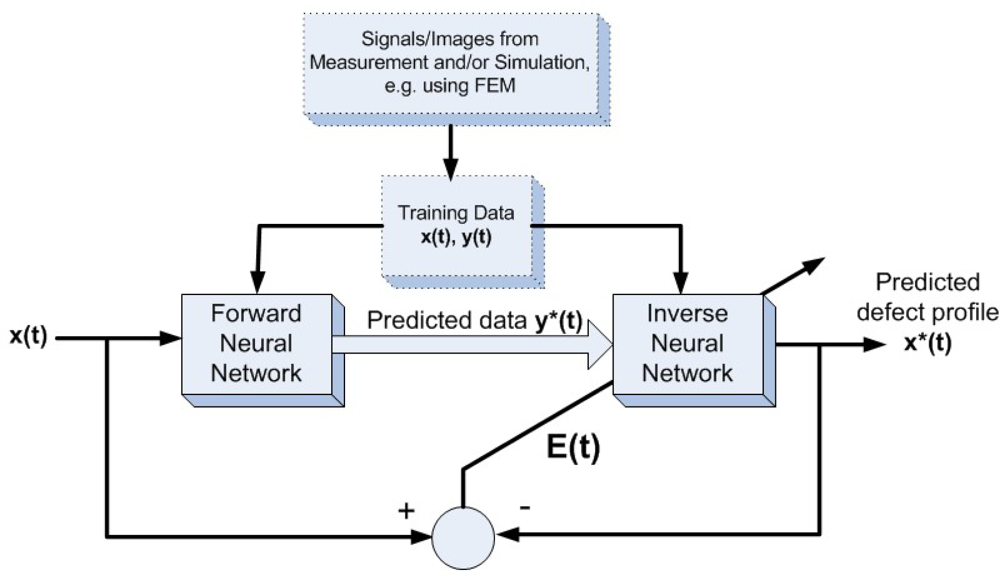
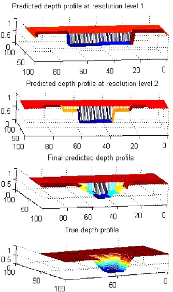
For image inversion techniques, the same group published two articles on MFL image reconstruction based on neural networks in 2002 and 2003 by Ramuhalli and Udpa [9,10]. In their papers, the radial basis function and wavelet basis function were first trained to approximate the mapping from the measured signal to the defect space, and the trained networks were used iteratively to estimate the defect profile. They extended their approach to the innovative multi-networks that are in feedback configuration and composed of a forward network and an inverse network. The schematic of the multi-networks are shown in Figure 4 with typical inversion results presented in [10]. Three-dimensional defect reconstruction for MFL imaging were further developed in 2006 by Joshi and Udpa based on the RBFNN approach with the coarse to fine results shown in Figure 5 [11].
Besides the efforts on those basis functions based forward and inverse methods, Haueisen et al. investigated both linear and nonlinear methods that include maximum entropy method (MEM), low resolution electromagnetic tomography (LORETA), L1 norm and L2 norm methods, to detect and characterize the MFL imaging data in early 2000s. Image reconstruction results using the above three methods were compared in their 2002 paper [12] concluding that the MEM, L1 norm and L2 norm methods usually performed well in MFL data inversion. However, in the authors’ opinion, both Udpa and Haueisen’s approaches suffer from the dependence on high and costly computational resources needed.
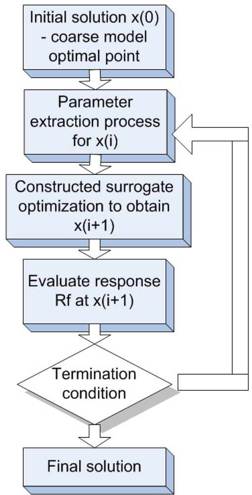
Recently, space mapping methodology(SMM) was proposed by Amineh et al. for defect characterization in MFL imaging, which is efficient due to the optimization burden shifts from a computationally expensive accurate or fine model to a less accurate or coarse model with faster speed. The simplified flowchart of the space mapping method is shown in Figure 6, the detailed SMM approach can be referred to the paper published in 2008 [13]. The challenge to achieve both fast computation or image processing and better interpretation of physics remains an active research topic.
Besides the image analysis and signal reconstruction for better interpretation and understanding of the MFL data, efforts on improving this magnetic imaging system itself have also been constant. In 2002, Parks proposed an optimum design to determine the size of the magnet in order to maximize the MFL signals and consequently generate superior MFL images [14]. The sensitivity of their optimum imaging system has been increased up to 200% and verified by measurement according to their findings. Their superior imaging results are shown in Figures 7 and 8. The authors do believe the next major breakthrough for MFL imaging should be initialized by development in innovative imaging instruments.
Most recently, a group in UK led by G.Y. Tian proposed to overcome the pitfalls of traditional MFL imaging by measuring the 3D magnetic field. Instead of the measurement of the two field components perpendicular to the testing surface (z axis) and parallel to the applied field (x axis), a high sensitivity three–axis magnetic field sensor was employed in their lab. Both finite element and experimental results demonstrated the merits of including additional information from the y axis. The 3D MFL imaging in Li and Tian’s work improved the defect characterization capabilities significantly, especially for irregular geometries. Both FE and experimental results were presented in 2007 [15].
Sophian et al. presented a new approach of imaging mechanism in 2006, termed as pulsed magnetic flux leakage (PMFL) method. Conventional MFL imaging techniques suffer in crack characterization such as sizing in the situations where defects take place on the near and far surfaces of the structures under inspection. Without introducing extra transducers or extra field components, like what Li and Tian proposed above, to overcome this problem, the PMFL clearly demonstrated advantages in terms of defect location and sizing by extracting features in time–frequency domain [16].
2.1.2. Electromagnetic Tomography Imaging
Eggleston et al. published one of the pioneering papers in 1990 on EM tomography imaging, who developed the electric current computed tomography for defect imaging in metals [17]. A variety of clinical and nonclinical applications were developed since then and the imaging method is well known as electrical impedance tomography (EIT). EIT seeks the electrical conductivity and permittivity inside a body or structures, given simultaneous measurements of electrical currents and potentials at the boundary. However, human imaging using EIT has gained a lot of attentions and achieved relative successes over those NDE imaging applications. One of the most cited articles was published in 1999 by Cheney et al., in which a survey on EIT and its mathematical model was extensively discussed [18]. Borcea et al. reviewed the theoretical and numerical studies for the inverse problems of EIT [19] in 2002. Another excellent review article on the pitfalls, challenges and developments of EIT imaging was published by Lionheart et al. in 2004 [20], which is worth mentioning. Similar imaging method, such as electrical resistive tomography(ERT), was also introduced and summarized in 2002 by Kemnaa et al., (for details, see [21]).
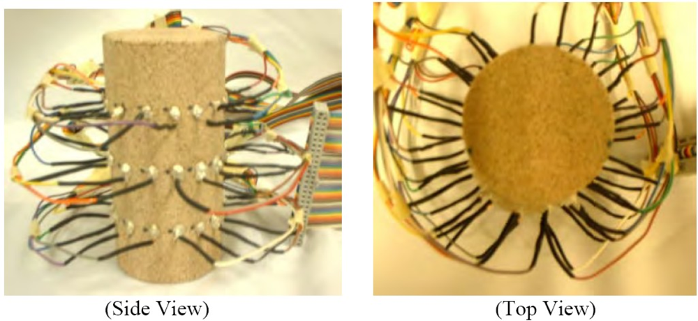
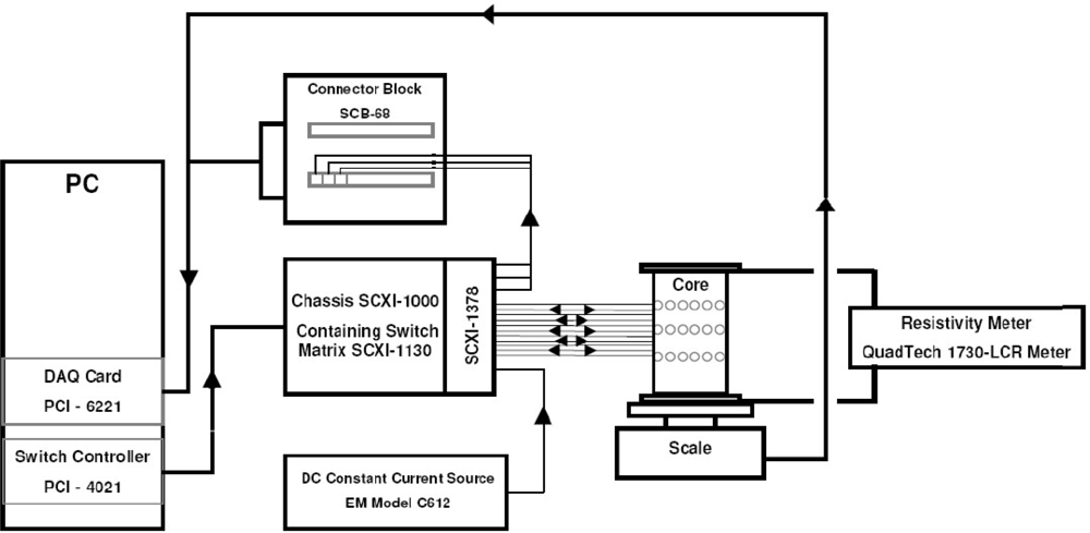
In the authors’ point of view, the three-dimensional EIT imaging is still in its infancy for nondestructive evaluation purposes. Stacey et al. at Stanford University published a technical report in 2006 on 3D EIT imaging that provides estimates of reservoir saturation at multiple scales by determining the resistivity distribution within the subsurface [22]. Although their system is limited to specific applications, their initial experimental results are promising, which used a Berea sandstone core with 48 electrodes attached in three rings of 16. The side and top view of electrode design is shown in Figure 9 and the EIT imaging system schematic is illustrated in Figure 10. To summarize their system, the voltage potential field was measured by applying a direct current pulse across the core and measuring the voltage potential at all electrodes, essentially applying the 4–wire resistance technique over all electrodes in turn. The PC cycles through the sequence by measuring the voltage potential at every electrode before changing the current source electrodes. The current is supplied by the data acquisition (DAQ) card. The scale and resistivity meter are used to calibrate the EIT measurements by providing the actual saturation and resistivity [22]. EIDORS toolkit, which was developed for applications to nonlinear and ill-posed inverse problem, was utilized. Experiments conducted by Stacey et al. have indicated that 3D EIT is a viable technique for studying the displacement characteristics of fluids with contrasting resistivity and is capable of detecting displacement fronts in near real-time. Again, in our perspective, EM tomography imaging techniques have been underestimated in NDE community and should be exploited more in future. More discussion will be conducted in the last section of this paper.
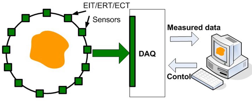
In contrast to EIT and ERT, electrical capacitance tomography (ECT) imaging attempts to image the permittivity distribution of an object by measuring the electrical capacitances between sets of electrodes placed around its periphery. Yang et al. reviewed the existing image reconstruction methods for ECT, including linear back-projection, singular value decomposition, Tikhonov regularization, Newton–Raphson, iterative Tikhonov, the steepest descent method, Landweber iteration, the conjugate gradient method, algebraic reconstruction techniques, simultaneous iterative reconstruction techniques and model-based reconstruction [23]. Figure 11 shows a typical EIT/ERT/ECT system with an multiple electrode sensor.
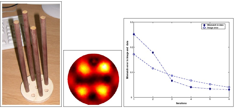
In addition to Yang’s comprehensive review paper on ECT reconstruction, Soleimani et al. studied the nonlinearity of the inverse permittivity problem of ECT and implemented a regularized Gauss–Newton for nonlinear image reconstruction with adoption of finite element method(FEM) as the forward model solver [24], recently in 2005. The ECT results of four plastic rods is shown in Figure 12. Soleimani and colleagues presented a Helmholtz type Regularization Method for ECT reconstruction in 2010 [25]. More recent literatures on ECT development can be referred to [26,27] and [28].
The other advances in magnetic based imaging other than the increasing in sensitivity include but are not limited to that, for example in 2004, Knauss et al. reported a high resolution, non-contact magnetic based current imaging technology localizing high resistance defects in packages to within 30 μm, an order of magnitude better than time domain reflectometry [29]. They also applied this novel imaging technique on various applications, such as present and next generation semiconductor devices by introducing the very low magnetic field [30].
2.2. Quasi-Static Imaging Methods
This section reviews the electromagnetic imaging methods with low excitation frequencies: quasi-static imaging techniques such as conventional eddy current imaging. Several hybrid imaging techniques utilizing eddy current are also summarized here including the EC-based magneto-optic (MO) imaging and EC-based giant magnetoresistive (GMR) imaging.
2.2.1. Eddy Current Imaging
Eddy current methods were initiated a few decades back and used extensively as one important electromagnetic NDE methods. Eddy current imaging is widely accepted as a nondestructive testing technique enabling efficient flaw reconstruction based on much richer and comprehensive data sets than the traditional Lissajous patterns obtained from a single EC scan [31]. Some of the pioneers, such as William Lord at Colorado State University in the 1980s, advanced both the theoretical and experimental aspects of EC imaging greatly [32–34]. In 1991, L. Udpa and S. S. Udpa co-authored a paper on neural networks based EC signals classification and the major contribution of their work was to introduce a rotation- and translation-invariant internal representation of the signals [35]. During the same year, Zorgati et al. published another pioneering paper on quantitative EC imaging of anomalies in conductive materials, which is the reflection mode diffraction tomography (DT) technique [36]. The applications of deterministic and stochastic quantitative inversion techniques to similar configurations were published later. Another early paper on EC imaging was published by Guettinger in 1993 [37].
Besides defect detection, material loss due to corrosion can also be imaged by eddy current and by assuming the linearized relationship between eddy current loop impedance change with the loss profile. Luong et al. developed a quantitative EC imaging system for corrosion detection and characterization in 1998 [38]. Numerical results using consistent data with noise are shown in Figure 13, which demonstrate the capability of the imaging system to accurately and quantitatively estimate the corrosion loss.
Understanding the physics and physical limits of eddy current imaging is always important. From both theoretical and experimental approaches, Auld et al. [39] and Albanese et al. [40] published during the same year of 1999 on eddy current modeling to understand how the eddy current energy interacting with the materials. Both the forward problem and inversion techniques were covered in their work. Blodgett and Nagy et al. investigated the lateral resolution limits of EC imaging in 2000 with results shown in Figures 14 and 15 [41]. They performed comparison between eddy current microscopy and acoustic microscopy results, which demonstrated the feasibility of high resolution EC imaging.
Also it is worthwhile to mention that innovative EC imaging sensors were continuously developed in the past two decades, such as array geometry invented for reconstruction of 3D flaw images by Gramz et al. in 1994 [31], orthogonal coils EC transducer proposed by Grimberg in 2000 [42] and the EC magnetic induction tomography (MIT) imaging system by Soleimani in 2006 [43]. Similar to the EIT in the static EM imaging category, the MIT tries to image the electrical conductivity of the target based on impedance measurements, however by injecting energy from pairs of EC excitation and generating images from detection coils.
Recently, a circular EC probe array geometry was introduced by Abascal in 2008, for the applications of measuring the variations of impedance data collected close to the inner surface of the metal tube, which can further characterize the locations and shapes of defects, such as inner, outer and through-wall void flaws [44]. As the readers can tell, new EC sensors will be on a track of continuously development at both academic institutions and commercial sectors. One most recent development is the rotating magnetic field probe design at Michigan State University (MSU) that were presented at the Quantitative Nondestructive Evaluation (QNDE) conference held in Burlington, VT in 2011.
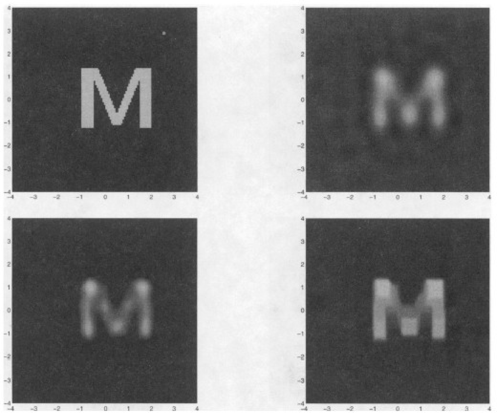
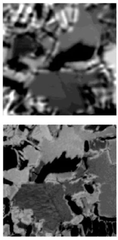
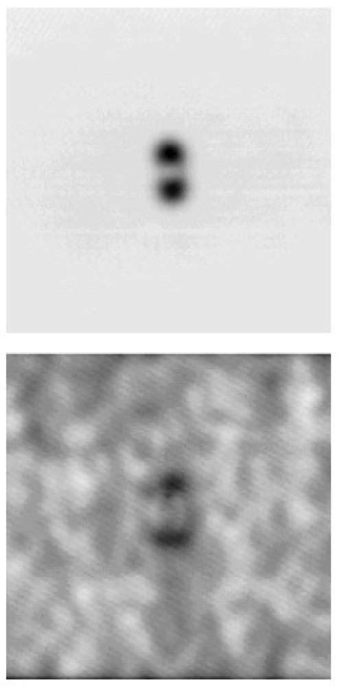
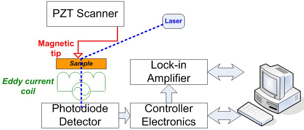
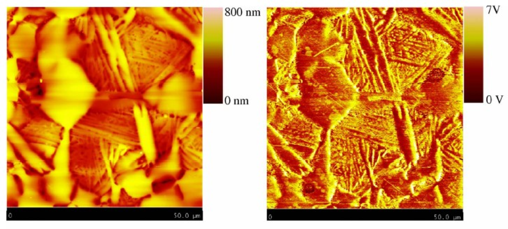
In 2008 and 2009, Nalladega et al. published an interesting paper and his doctoral dissertation [45], respectively, on a high resolution electrical conductivity imaging technique based on the principles of eddy current and atomic force microscopy (AFM). In the imaging system that he proposed, an electromagnetic coil is used to generate eddy currents in an electrically conducting material. The eddy currents generated in the conducting sample are detected and measured with a magnetic tip attached to a flexible cantilever of an AFM [46]. The contrast in the image was explained based on the electrical conductivity and eddy current force between the magnetic tip and the sample, where the spatial resolution of the eddy current imaging system was determined by imaging carbon nanofibers in a polymer matrix. The schematic of this high resolution eddy current microscopy is illustrated in Figure 16 with imaging results shown in Figure 17 [47].
2.2.2. Pulsed Eddy Current Methods
Pulsed Eddy Current (PEC) Imaging was initially proposed during the early 1990s but bloomed during the past decade [48–50]. PEC imaging takes advantage of the broad frequency spectrum of an short excitation pulse in time domain over the conventional single frequency EC imaging.
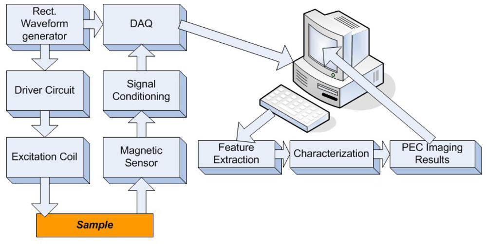
The early pulsed eddy current sensors usually extracted defect information from the peak values and temporal profiles of the signals. Tian et al. proposed a prototype of pulsed eddy-current imaging with multiple sensors and used the principal component analysis (PCA)-based feature extraction that provides orthogonal information [51]. The schematic of a typical PEC imaging system is shown in Figure 18.
In 2010, the authors and their colleagues Yang et al. developed a novel PEC–GMR imaging technique by integrating the giant magnetoresistive field sensor for the detection and characterization of buried cracks in multiple layered structures [52]. The PEC–GMR system is illustrated in Figure 19 and typical imaging results shown in Figure 20.
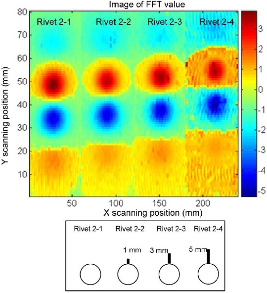
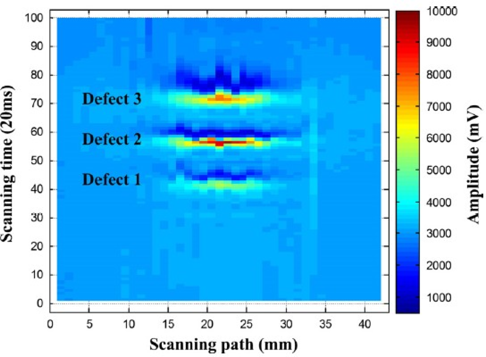
A different excitation coil structure with rectangular shape was proposed by He et al. in 2011 and various C–scan images were obtained for the buried subsurface defects. The top view of the PEC probe can be seen in Figure 21 and their sample PEC images were shown in Figure 22 for three different crack sizes [53].
2.2.3. Eddy Current Magneto-Optic Imaging
In order to achieve faster imaging speed with higher image resolution, several EC-based hybrid imaging techniques were developed. One of the most successful methods among them is the magneto-optic (MO) imaging technique invented by Shih and Fitzpatrick in the early 1990s [54]. The magneto-optic imager (MOI) is widely used in detecting surface and subsurface cracks and corrosion in aircraft skins. The instrument provides analog images of the anomalies based on eddy current induction techniques and an MO sensor using the Faraday rotation effect. The schematic of the EC–MOI system is shown in Figure 23.
The merits of the MOI that make it attractive include rapid and large-area inspection, insensitivity to liftoff variations, and easy interpretation in contrast to the complex impedance data of conventional eddy current inspections [55]. Fan and Deng et al. developed a real-time aircraft rivet imaging, crack detection and classification system implemented on a TMS320C6000 DSP platform in 2006 and demonstrated at Kuka Robotics in Detroit, 2007. Their system can not only reduce the detection variability from inspector to inspector but also have the capability of fully automated image analysis, such as segmentation, enhancement (noise removal), quantization and classification [56]. A quantitative basis for MO image processing and characterization was established by Deng et al. during the same year by introducing the skewness functions. Meanwhile, to understand the MO imaging physics, a numerical simulation model that produces quantitative values of the magnetic fields associated with induced eddy currents interacting with structural defects using 3D FEM simulation was presented by Zeng et al. [57], which is an essential complement to the instrument development process. This eddy current based hybrid technique became a great success. The dynamic collaborative research team among government, industries and academia including the authors was awarded the 2005 FAA-ATA Better Way Award because of their contributions in the MOI technique. This state-of-the-art system can be used by mounting the MO imager on a robot for fully automated scanning.
In 2006, one similar system named linear MO imager (LMOI) was patented in Europe by Joubert et al., which consists of the combination of a dedicated MO sensor featuring a linear and hysteresis-free magnetization loop, used with an original image acquisition system based on a stroboscopic approach, and a specific high sensitivity eddy current inductor [58]. The first schematic of the LMOI integrated prototype is shown in Figure 24, which is similar to the setup of the pioneering MOI system by Shih and Fitzpatrick. The field of view of Joubert’s LMOI system, in contrast to the US version, is circular as imaging results shown in Figure 25. This research group published another two articles in 2009 and 2010 for characterization of subsurface defects in aeronautical riveted lap joints using a multi-frequency imaging setting [59,60]. Further improvement on magneto-optic based imaging methods explored new sources of optical energy. Instead of using polarized light, Cheng et al. adopted laser and combined with MO thin films technology to achieve an enhanced MO imaging system in 2007 [61].
2.2.4. Eddy Current Magnetoresistive Imaging
Another hybrid EC imaging utilized the Nobel-winning discovery, giant magnetoresistive effect, and measured the 3D magnetic field generated by the eddy current perturbation directly. The use of giant magnetoresistive (GMR) sensors for electromagnetic imaging in nondestructive evaluation has grown considerably in the last few years. A key advantage of GMR sensors is a flat frequency response extending from DC to hundreds of MHz, making them particularly attractive for low-frequency and multi-frequency eddy current detection [62].
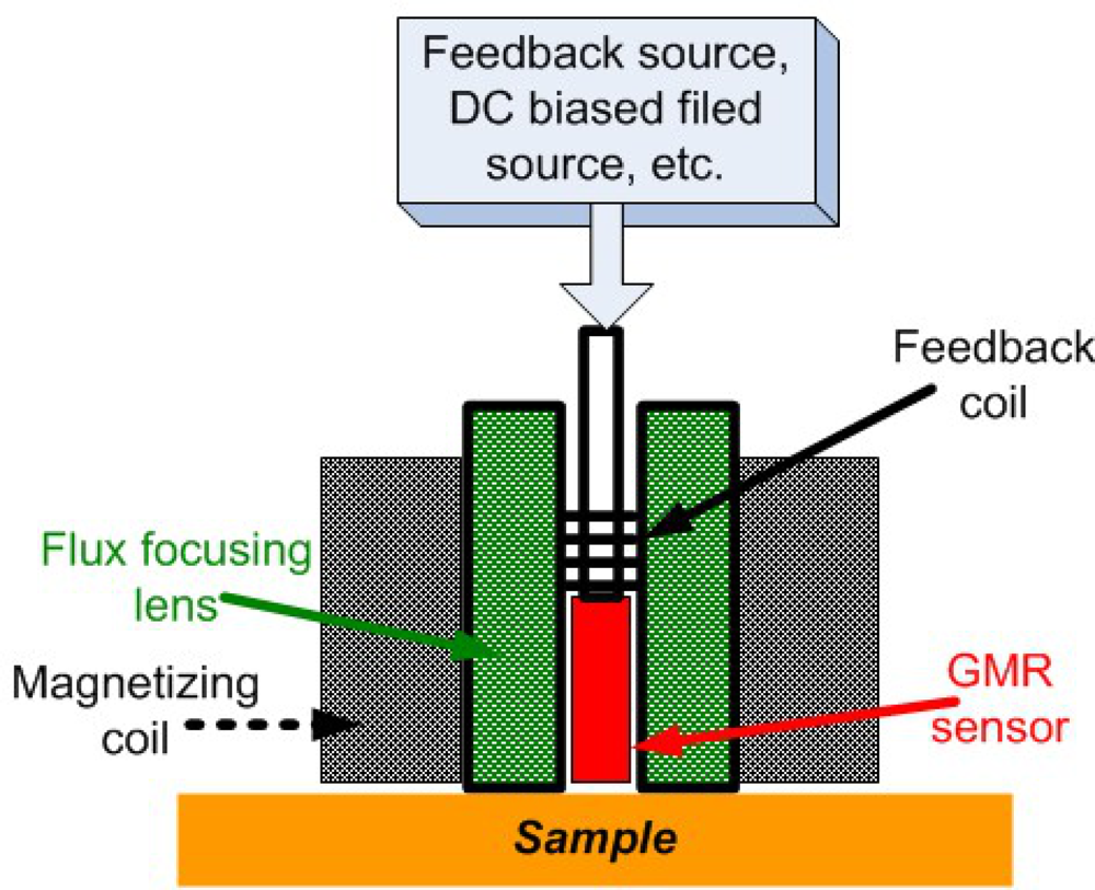
For EC imaging, there is always a trade-off between the penetration depth due to skin depth effect and better image resolution that is directly related to frequency. In particular, the low frequency sensitivity of the GMR provides a practical means to perform electromagnetic inspections on thick layered conducting structures. Wincheski et al. at NASA Langley Research Center incorporated a commercially available GMR sensor into the self-nulling probe and their research showed that this imaging set up can greatly enhance the low frequency capabilities of the imaging device. By combining with image processing, their system has resulted in a greatly improved signal-to-noise ratio (SNR) for very deeply buried flaws in conducting materials [63]. Figure 26 shows an illustration of their system schematic.
If the readers want more background knowledge on magnetoresistive physics, one excellent review article on magnetoresistive imaging sensors was published by Jander in 2005, in which the physical principles, manufacturing process, and performance characteristics of the three main types of MR devices, anisotropic magnetoresistance (AMR), giant magnetoresistance (GMR) and tunneling magnetoresistance (TMR) are thoroughly discussed [62].
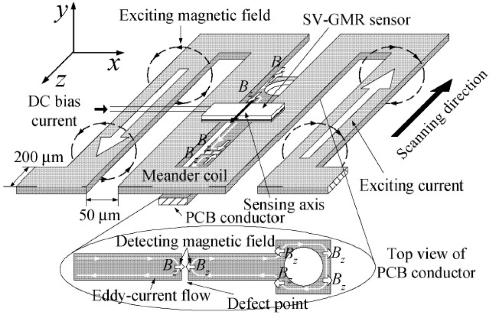
In the year of 2006, Yamada et al. proposed a needle type GMR imaging technique, SV–GMR system and the applications of this new sensor including the inspection of bare printed circuit board and the measurement of the density of magnetic fluid injected in living body for the hyperthermia treatment [64]. The SV–GMR imaging system schematic is shown in Figure 27. Singh and Raj et al. developed another novel imaging system involved both GMR sensors and MFL principles for detection of various near side notches and far side notches in a 12 mm thick carbon steel [65]. At NDE lab of Michigan State University, a flexible and efficient real-time GMR imaging system for nondestructive evaluation of aircraft was developed by Nair et al. with several advantages over the past prototypes [66]. The reader can find other similar types of EC-GMR system that were developed within the last decades, for example the system by Postolache et al. published in 2008 [67] or Tsukada system in 2006 [68], etc.
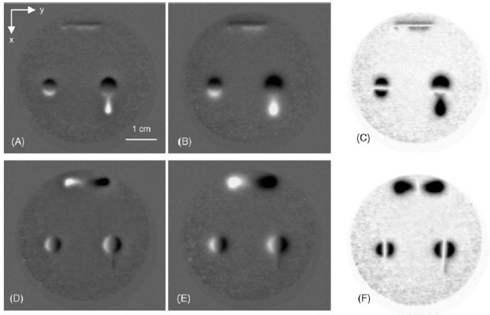
Due to the low operating frequency and subsequent noisy signals, the EC–GMR image processing and analysis is always critical and challenging. Numerous efforts have been put into this problem, and in 2009, Deng et al. introduced the optimum detection angle (ODA) to combine the in-phase and quadrature components of GMR signals, enhanced the GMR image data by over ten orders of magnitude in SNR [69]. Kim et al. developed a PEC–GMR imaging platform in 2010 and proposed a principle component analysis (PCA) based feature extraction and classification algorithm for those data [70], which took advantage of both pulsed excitation and sensitive GMR sensors. Most recently, Zeng et al. published several quantitative metrics for characterizing EC–GMR images and the improvement in probability of detection(POD) was clearly demonstrated [71].
2.2.5. Other Low Frequency EM Imaging Sensors
Other EM imaging sensors that fall into this low frequency category include, but are not limited to, magnetic induction tomography (MIT), giant magneto-impedance (GMI) imaging, which will be briefly introduced in this review article. MIT applies a magnetic field from an excitation coil to induce eddy currents in the material, and the magnetic field is then detected by sensing coils [72]. Griffiths et al. discussed the physics of MIT as a fascinating and new imaging modality for both industry and medical imaging, also the challenges in acquiring good quality MIT data in 2001.
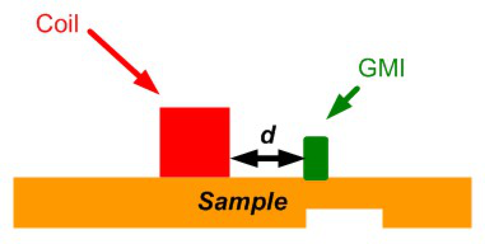
Vachera et al. developed a high sensitivity imaging sensor based on GMI effect that combines good sensitivity performances at low frequencies and small size of sensors in 2007 [73]. A simple configuration of GMI imaging is shown in Figure 28.
2.3. High Frequency Time Varying Imaging Methods
High frequency time-varying EM imaging methods are discussed in this section. In contrast to the static and low frequency EM imaging modalities, they have their unique advantages and specific applications.
2.3.1. Microwave Imaging
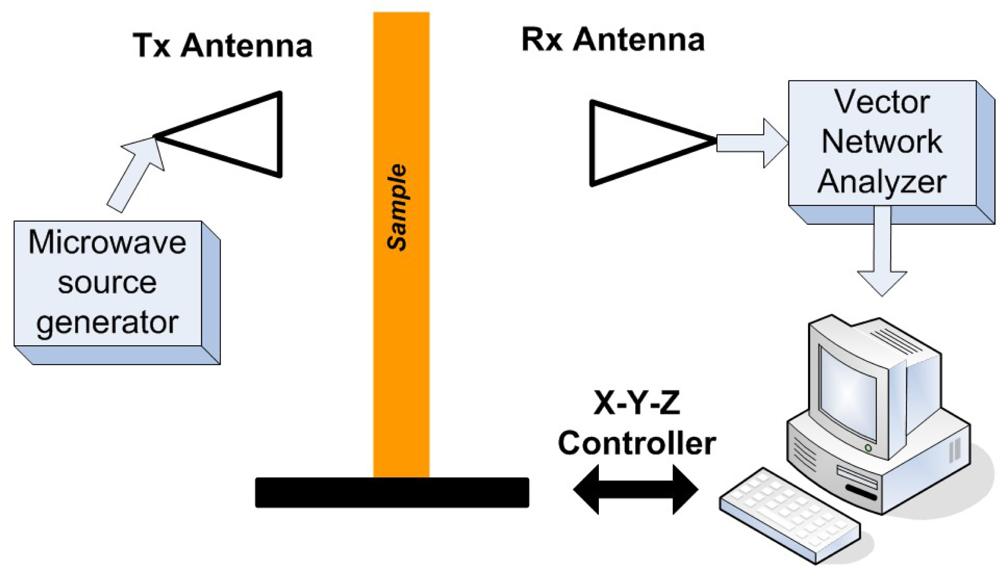
For the past a few decades, the tremendous advances of microwave NDE imaging is clearly one proof of the importance of EM imaging within this high frequency band. Several articles in the late 1980s and early 1990s foresaw the potential and a growing field of applications in microwave sensing, especially for nondestructive evaluation [74–76]. An excellent review on this topic was given by Zoughi et al. in the year of 2007 [77]. Examples of the state-of-the-art microwave imaging for various applications, such as inspection of Carbon Fibre Reinforced Polymer (CFRP) composite laminate strengthened structures, detection and evaluation of corrosion and precursor pitting under paint, etc., were covered in this article. However, Zoughi stated that the inadequate commercial availability of microwave systems for NDE purposes has limited its more extensive implementation. The authors do believe and expect microwave imaging to be one of the most dominant and versatile NDE imaging techniques in the near future. A typical but simple microwave imaging system setup can be seen in Figure 29 [78].
In 1995, Diener et al. studied an imaging system with an open-ended waveguide at the frequency of 30 GHz for evaluation of dielectric materials. He compared the results obtained from microwave energy with the more prominent NDE methods at that time such as ultrasonics, X-rays and thermal waves and demonstrated the great performance of microwave imaging [79]. Another driving force for this technique lies in the biomedical applications and clinical imaging needs, for example, the breast cancer imaging and biological tissue characterization [80] utilize the microwave energy extensively. These medical related literatures will not be elaborated in this paper but are worth mentioning since it is another active research field of microwave imaging nowadays.
Another major application of microwave imaging is to determine the shape and location of an buried object or defect from the measurements of the field scattered by the object or defect. Underground object detection research has undergone a long way with numerous applications. Ground penetrating radar (GPR) techniques have been thoroughly studied and developed. Belkebir et al. proposed a microwave imaging system and tested two different reconstruction algorithms, a Newton–Kantorovich (NK) method and the modified gradient (MG) method by comparing their effectiveness and robustness [81]. In 1999, Tabib-Azar et al. imaged and mapped material non-uniformities and defects using microwave generated at the end of a micro-stripline resonator with 0.4 mm lateral spatial resolution at 1 GHz. They introduced a novel sensor called evanescent microwave probe (EMP) and demonstrated the overall capabilities of EMP imaging techniques as well as discussed various probe parameters that can be used to design EMPs for different applications [82].
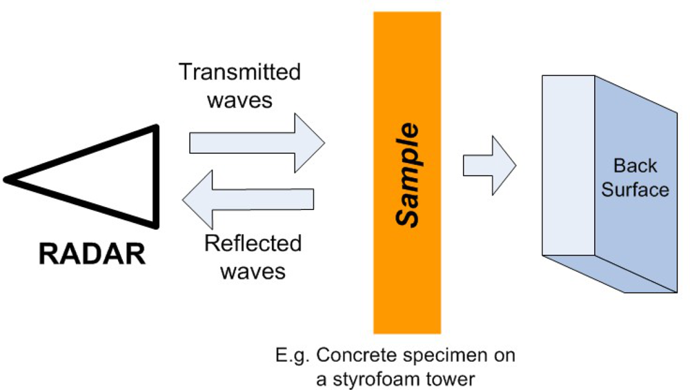
Critical infrastructure monitoring and inspection is always a challenging problem. Radar imaging has become a powerful and effective tool for the nondestructive testing of concrete structures. Weedon et al. proposed a step-frequency radar imaging system in 1994 [76]. An advancement of the method can be achieved through the understanding of the interaction between electromagnetic waves and concrete, and the identification of optimum radar measurement parameters for probing concrete [83]. Figure 30 is a simple radar imaging experimental system setup. Rhim et al. developed a wide band imaging radar to obtain 2D and 3D imagery of concrete targets.Three different types of internal configurations were imaged. For the determination of optimum parameters after systematic radar measurements, they found that 2 to 3.4 GHz waveforms are adequate for the concrete thickness measurement, 3.4 to 5.8 GHz waveforms are adequate for the detection of delamination, and 8 to 12 GHz waveforms are adequate for the detection of inclusions embedded inside concrete [83]. Rhim, in the year of 1998, also published the concrete materials characterization results using electromagnetic frequencies from 0.1 to 20 GHz that will serve as a basis in applying wide band microwave imaging techniques for NDE of concrete using radar [84].
In 2004, Pastorino summarized the development of efficient inverse scattering based procedures for electromagnetic imaging at microwave frequencies, especially for 2D tomographic imaging approach. He also introduced the modulated scattering technique, which is a promising technique strongly related to electromagnetic scattering concepts [78]. The modulated scattering system schematic is shown in Figure 31.
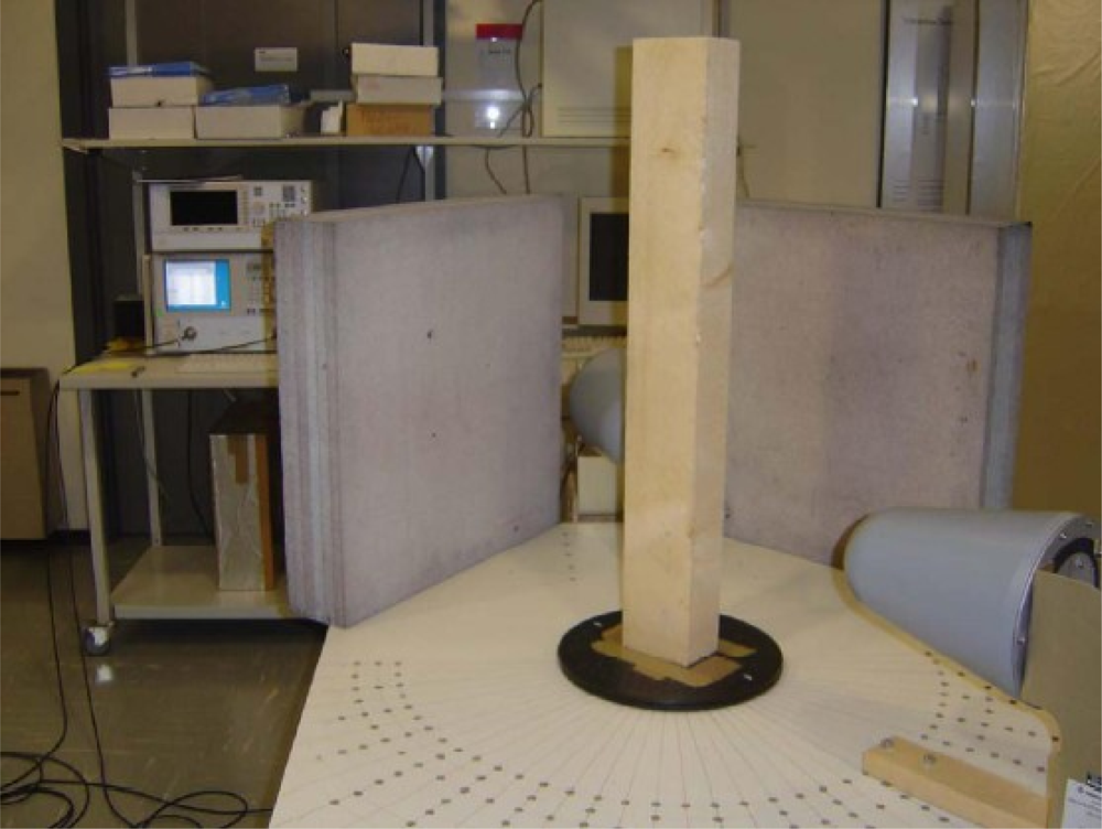
In [85], Pastorino extensively reviewed the stochastic optimization methods applied to microwave imaging with various imaging modalities considered, such as tomography, buried object detection and borehole sensing. Pastorino et al. also presented an experimental setup based on interrogating microwaves to obtain images of the cross section of dielectric cylinders. Both experimental results and numerical validations have been conducted. Figures 32 and 33 show the system schematic and experimental setup, respectively.
In the years of 2003 and 2004, Caorsi et al. proposed a hybrid genetic algorithm (GA) based microwave imaging procedure for detecting defects in dielectric structures by pre-computing the Green’s function for the configuration without defects and consequently saving significant imaging and reconstruction time [86,87], which was considered as a big improvement in microwave imaging inversion.
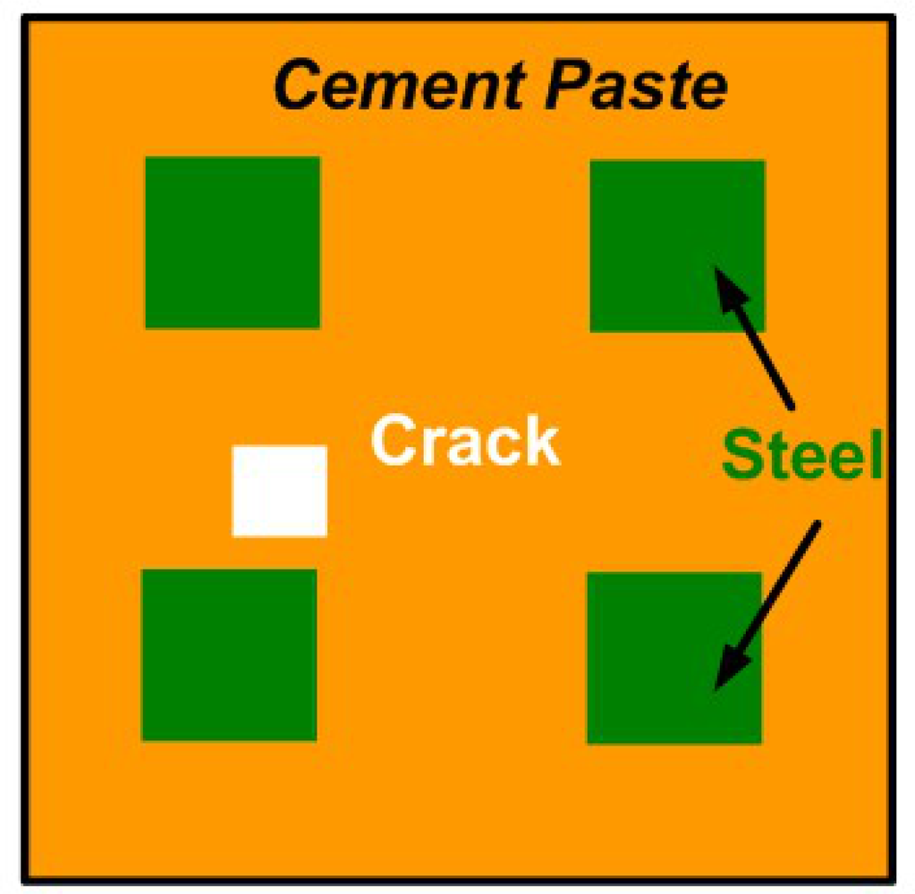
Similar types of efforts were carried out by Benedetti et al., who developed an innovative inversion procedure based on the use of GA and on the Sherman–Morrison–Woodbury (SMW) matrix inversion method [88,89] with the testing structure shown in Figure 34. Also, Massa et al. from the same group presented the improved tomographic microwave imaging approach based on the use of the SMW updating formula for electric field computation with applications in civil structures. Donelli and Massa et al. in 2005 developed another innovative stochastic algorithm called the particle swarm optimizer (PSO) for the solution of microwave inverse scattering problem [90]. In 2011, this group tried to solve the 2D inverse scattering problem by probing the unknown scenarios with TE and TM waves with multi-zooming approach [91]. Besides those literatures, there is another excellent technical article published in 2006 by Langenberg et al., who tried to unify the theory of electromagnetic, acoustic and elastic wave fields for imaging purposes with examples of bridge NDE [92].
Zoughi et al. conducted pioneering research in microwave imaging at the Missouri University of Science and Technology (known as University of Missouri–Rolla before) and he published a review paper in 2008 on the near-field microwave imaging demonstrating the capabilities of EM imaging for detecting cracks and evaluating their various dimensional properties including determining a crack tip location accurately [93] at time varying frequencies. Recently, Wu et al. presented the development of an experimental microwave tomography system intended for oil and gas flow measurements in 2009 [94].
2.3.2. Millimeter Wave Imaging and Terahertz Imaging
Millimeter wave imaging or terahertz (THz) imaging has drawn more and more attention in recent years. The implementation of THz imaging for nondestructive evaluation shows great promise in 2D and 3D non-contact inspection of non-conductive materials such as plastics, foam, composites, ceramics, paper, wood and glass [95]. For a review of these high frequency NDE imaging techniques, the readers can refer to the paper by Kharkovsky et al. published in 2007 [77].
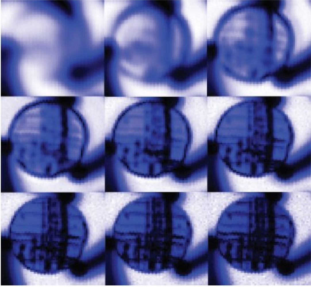
Similar to the efforts in high resolution EC imaging methods, Hor et al. in 2008 examined the cork’s surface and interior using this short wavelength and achieved roughly 100 to 300 μm resolution for the presence of voids, defects and changes in grain structures [96]. Their results can be seen in Figure 35.
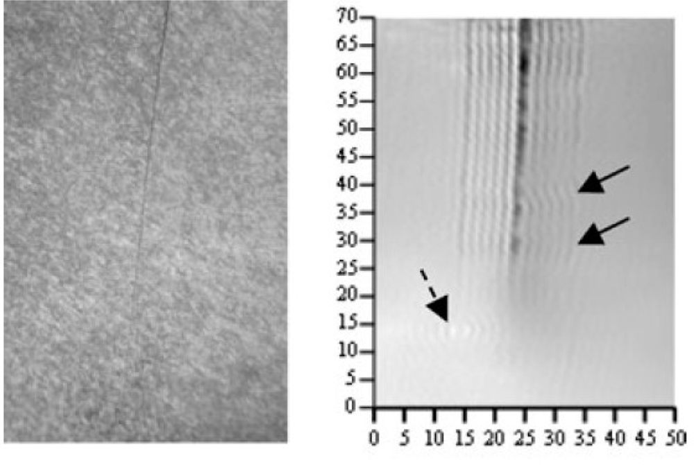
Zoughi et al. have successfully applied millimeter wave techniques on nondestructive detection and evaluation of stress-induced fatigue cracks in metals working in several critical environments including surface transportation (steel bridges, railroad tracks, railroad car wheels, etc.), aerospace transportation (aircraft fuselage, landing gears, etc.) and power plants (steam generator tubings, etc.) [93]. See Figure 36 for the comparison between the images obtained from microscope and the 90 GHz microwave imaging system. In 2009, Kharkovsky, who works with Zoughi, evaluated the efficacy of near-field millimeter-wave NDE techniques, using open-ended flange-mounted rectangular waveguide probes [97]. Because of the ability to penetrate through dielectric substances, Kemp et al. published the development of a millimeter and sub-millimeter continuous wave system for imaging corrosion pitting, structural defects and beat damage in common aircraft materials such as aluminum and polyamides in 2010 [98].
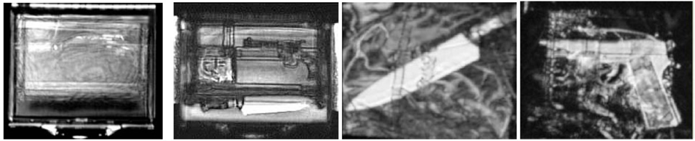
On the other hand, for polymer materials, Beckmann et al. proposed to use THz frequencies from 0.05 to 2 THz to detect flaws in those materials like degradation areas in polymer pipelines, moisture distributions and de-laminations in composites used in aircraft industry [99]. In 2005, Zimdars et al. reported on the applications of a transmission and reflection reconfigurable large area time domain THz imager for homeland security and NDE applications [95,100]. See Figure 37 for their results of co-linear THz reflection imaging. Other imaging system development effort includes: a compact sub-THz imaging system that was presented by Oyama et al. for the application of inspecting timbers, concrete and ceramic tiles [101]. The most recent progress in general THz science and technology can be found in the review article authored by the researchers at RPI [102] and in another outstanding review paper by Bogue et al. in 2009 that provided a detailed insight into the present state of THz imaging [103].
2.4. Other EM Imaging Methods and Inverse Problems
It is neither a possibility nor our intention to complete an exhaustive search on all the EM imaging methods literatures for NDE applications. However, a comprehensive coverage of most of the major EM NDE imaging methods is our objective for this article and in this paragraph, we briefly introduce several other EM imaging methods that are important to NDE community, such as: the super-conducting quantum interference device (SQUID) imaging for NDE [104–106]; magneto-acoustic imaging [107,108]; millimeter acoustic imaging [109]; microwave induced thermoacoustic imaging [110]; and general EM tomography imaging techniques [111–115]. The inversion of EM NDE imaging is a separate but very comprehensive topic. If interested, the readers can refer to the following articles for more information [116–121].
3. Summary and Conclusions
A comprehensive and up-to-date review of electromagnetic imaging methods for NDE applications has been conducted in this article. The recent advances in sensing technology, hardware and software development dedicated to imaging, image processing and material sciences have greatly expanded the application fields, sophisticated the systems design and made the potential of electromagnetic NDE imaging seemingly unlimited. Like the research and development in other imaging techniques, there are always trade-off and hurdles for us in achieving both higher image resolution/SNR and lower noise, faster image acquisition and reasonably good image quality, etc. It is believed that the emerging technologies in computer engineering will significantly impact the EM NDE imaging development. For instance, by introducing the graphics processing units (GPU), it will not only redefine the computational related works for many imaging methods we mentioned above, but also push the development of imaging sensors forward through parallel data processing, fast image acquisition, enhancement and compression. The authors foresee that there is great potential and future development in the field of EM imaging for NDE and SHM applications, including both active and passive sensors.
References
- Tricoles, G.; Farhat, N.H. Microwave holography: Applications and techniques. Proc. IEEE 1977, 65, 108–121. [Google Scholar]
- Deng, Y. Forward and Inverse Problems in Noninvasive Imaging Techniques. Ph.D. Thesis,. Michigan State University, East Lansing, MI, USA, 2009. [Google Scholar]
- Zhu, Y.K.; Tian, G.Y.; Lu, R.S.; Zhang, H. A review of optical NDT technologies. Sensors 2011, 11, 7773–7798. [Google Scholar]
- Achenbach, J. Quantitative nondestructive evaluation. Int. J. Solids Struct 2000, 37, 13–27. [Google Scholar]
- Jiles, D.C. Review of magnetic methods for nondestructive evaluation. NDT Int 1988, 21, 311–319. [Google Scholar]
- Jiles, D. Review of magnetic methods for nondestructive evaluation (Part 2). NDT Int 1990, 23, 83–92. [Google Scholar]
- Mandayam, S.; Udpa, L.; Udpa, S.S.; Lord, W. Wavelet-based permeability compensation technique for characterizing magnetic flux leakage images. NDT&E Int 1997, 30, 297–303. [Google Scholar]
- Afzal, M.; Udpa, S. Advanced signal processing of magnetic flux leakage data obtained from seamless gas pipeline. NDT&E Int 2002, 35, 449–457. [Google Scholar]
- Ramuhalli, P.; Udpa, L.; Udpa, S.S. Electromagnetic NDE signal inversion by function-approximation neural networks. IEEE Trans. Magn 2002, 38, 3633–3642. [Google Scholar]
- Ramuhalli, P.; Udpa, L.; Udpa, S.S. Neural network-based inversion algorithms in magnetic flux leakage nondestructive evaluation. J. Appl. Phys 2003, 93, 8274–8276. [Google Scholar]
- Joshi, A.; Udpa, L.; Udpa, S.; Tamburrino, A. Adaptive wavelets for characterizing magnetic flux leakage signals from pipeline inspection. IEEE Trans. Magn 2006, 42, 3168–3170. [Google Scholar]
- Haueisen, J.; Unger, R.; Beuker, T.; Bellemann, M.E. Evaluation of inverse algorithms in the analysis of magnetic flux leakage data. IEEE Trans. Magn 2002, 38, 1481–1488. [Google Scholar]
- Amineh, R.K.; Koziel, S.; Nikolova, N.K.; Bandler, J.W.; Reilly, J.P. A space mapping methodology for defect characterization from magnetic flux leakage measurements. IEEE Trans. Magn 2008, 44, 2050–2065. [Google Scholar]
- Park, G.S.; Park, E.S. Improvement of the sensor system in magnetic flux leakage-type Nondestructive Testing (NDT). IEEE Trans. Magn 2002, 38, 1277–1280. [Google Scholar]
- Li, Y.; Wilson, J.; Tian, G.Y. Experiment and simulation study of 3D magnetic field sensing for magnetic flux leakage defect characterisation. NDT&E Int 2007, 40, 179–184. [Google Scholar]
- Sophian, A.; Tian, G.Y.; Zairi, S. Pulsed magnetic flux leakage techniques for crack detection and characterisation. Sens. Actuat. A 2006, 125, 186–191. [Google Scholar]
- Eggleston, M.R.; Schwabe, R.J.; Isaacson, D.; Coffin, L.F. The application of electric current computed tomography to defect imaging in metals. Rev. Prog. Quant. NDE 1990, 9, 455–462. [Google Scholar]
- Cheney, M.; Isaacson, D.; Newell, J.C. Electrical impedance tomography. SIAM Rev 1999, 41, 85–101. [Google Scholar]
- Borcea, L. Electrical impedance tomography. Inverse Probl 2002, 18, R99–R136. [Google Scholar]
- Lionheart, W.R.B. EIT reconstruction algorithms pitfalls, challenges and recent developments. Physiol. Meas 2004, 25, 125–142. [Google Scholar]
- Kemnaa, A.; Vanderborghta, J.; Kulessab, B.; Vereecken, H. Imaging and characterisation of subsurface solute transport using electrical resistivity tomography (ERT) and equivalent transport models. J. Hydrol 2002, 267, 125–146. [Google Scholar]
- Stacey, R.W. Electrical Impedance Tomography; Technical Report SGP-TR-182; The Department of Petroleum Engineering, Stanford University: Stanford, CA, USA, 2006. [Google Scholar]
- Yang, W.; Peng, L. Image reconstruction algorithms for electrical capacitance tomography. Meas. Sci. Technol 2003, 14, R1–R13. [Google Scholar]
- Soleimani, M.; Lionheart, W.R.B. Nonlinear image reconstruction for electrical capacitance tomography using experimental data. Meas. Sci. Technol 2005, 16, 1987–1996. [Google Scholar]
- Soleimani, M.; Yalavarthy, P.K.; Dehghani, H. Helmholtz-type regularization method for permittivity reconstruction using experimental phantom data of electrical capacitance tomography. IEEE Trans. Instrum. Meas 2010, 59, 78–83. [Google Scholar]
- Marashdeh, Q.; Warsito, W.; Fan, L.S.; Teixeira, F.L. Nonlinear forward problem solution for electrical capacitance tomography using feed forward neural network. IEEE Sens. J 2006, 6, 441–449. [Google Scholar]
- Marashdeh, Q.; Warsito, W.; Fan, L.S.; Teixeira, F.L. A multimodal tomography system based on ECT sensors. IEEE Sens. J 2007, 7, 426–433. [Google Scholar]
- Martinez, Olmos M.; Carvajal, M.A.; Morales, D.P.; Garcia, A.; Palma, A.J. Development of an electrical capacitance tomography system using four rotating electrodes. Sens. Actuat. A Phys 2008, 148, 366–375. [Google Scholar]
- Knauss, L.A.; Orozco, A.; Woods, S.I.; Wang, Z. Advances in Magnetic-Based Current Imaging for High Resistance Defects and Sub-Micron Resolution. Proceedings of the 11th International Symposium on the Physical and Failure Analysis of Integrated Circuits, (IPFA’04), Hsinchu, Taiwan, 5–8 July 2004; pp. 267–270.
- Knauss, L.; Woods, S.; Orozco, A. Current imaging using magnetic field sensors. Microelectron. Fail. Anal 2004, 1, 303–311. [Google Scholar]
- Gramz, M.; Stepinski, T. Eddy current imaging, array sensors and flaw reconstruction. Res. Nondestruct. Eval 1994, 5, 157–174. [Google Scholar]
- Udpa, S.S. Parametric Signal Processing for Eddy Current NDT. Ph.D. Thesis,. Colorado State University, Fort Collins, CO, USA, 1983. [Google Scholar]
- Udpa, L. Imaging of Electromagnetic NDT Phenomena. Ph.D. Thesis,. Colorado State University, Fort Collins, CO, USA, 1986. [Google Scholar]
- Udpa, L.; Lord, W. Search based imaging technique for electromagnetic NDT. Proc. IEEE 1989. [Google Scholar]
- Udpa, L.; Udpa, S.S. Neural Networks for the Classification of Nondestructive Evaluation Signals. IEE Proc-F Rad. Sig. Proc 1991, 138, 41–45. [Google Scholar]
- Zorgati, R.; Duchene, B.; Lesselier, D.; Pons, F. Eddy current testing of anomalies in conductive qualitative materials part I: Quantitative imaging via diffraction tomography techniques. IEEE Trans. Magn 1991, 27, 4416–4437. [Google Scholar]
- Guettinger, T.W.; Grotzn, K.; Wezel, H. Eddy current imaging. Mater. Eval 1993, 51, 444–451. [Google Scholar]
- Luong, B.; Santosa, F. Quantitative imaging of corrosion in plates by eddy current methods. SIAM J. Appl. Math 1998, 58, 1509–1531. [Google Scholar]
- Auld, B.A.; Moulder, J.C. Review of advances in quantitative eddy current nondestructive evaluation. J. Nondestruct. Eval 1999, 18, 3–36. [Google Scholar]
- Albanese, R.; Rubinacci, G.; Villoney, F. An integral computational model for crack simulation and detection via eddy currents. J. Comput. Phys 1999, 152, 736–755. [Google Scholar]
- Blodgett, M.; Hassan, W.; Nagy, P.B. Theoritical and experimental investigations of the lateral resolution of eddy current imaging. Mater. Eval 2000, 58, 647–654. [Google Scholar]
- Grimberg, R.; Savin, A.; Radu, E.; Mihalache, O. Nondestructive evaluation of the severity of discontinuities in flat conductive materials by an eddy-current transducer with orthogonal coils. IEEE Trans. Magn 2000, 36, 299–307. [Google Scholar]
- Soleimani, M.; Lionheart, W.R.B.; Peyton, A.J.; Ma, X.; Higson, S.R. A three-dimensional inverse finite-element method applied to experimental eddy-current imaging data. IEEE Trans. Magn 2006, 42, 1560–1567. [Google Scholar]
- Abascal, J.F.P.J.; Lambert, M.; Lesselier, D.; Dorn, O. 3-D eddy-current imaging of metal tubes by gradient-based, controlled evolution of level sets. IEEE Trans. Magn 2008, 44, 4721–4729. [Google Scholar]
- Nalladega, V. Design and Development of Scanning Eddy Current Force Microscopy for Characterization of Electrical, Magnetic and Ferroelectric Properties with Nanometer Resolution. Ph.D. Thesis,. University of Dayton, Dayton, OH, USA, 2009. [Google Scholar]
- Nalladega, V.; Sathish, S.; Jata, K.V.; Blodgett, M.P. High resolution eddy current imaging with atomic force microscope. Rev. Quant. Nondestruct. Eval 2008, 27, 400–406. [Google Scholar]
- Nalladega, V.; Sathish, S.; Jata, K.V.; Blodgett, M.P. Development of eddy current microscopy for high resolution electrical conductivity imaging using atomic force microscopy. Rev. Sci. Instrum 2008, 79, 1–11. [Google Scholar]
- Dai, X.; Ludwig, R.; Palanisamy, R. Numerical simulation of pulsed eddy current nondestructive testing phenomena. IEEE Trans. Magn 1990, 26, 3089–3096. [Google Scholar]
- Bowler, J.; Johnson, M. Pulsed eddy-current response to a conducting half-space. IEEE Trans. Magn 1997, 33, 2258–2264. [Google Scholar]
- Giguere, S.; Lepine, B.A.; Dubois, J.M.S. Pulsed eddy current technology: Characterizing material loss with gap and lift-off variations. Res. Nondestruct. Eval 2001, 13, 119–129. [Google Scholar]
- Tian, G.Y.; Sophian, A.; Taylor, D.; Rudlin, J. Multiple sensors on pulsed eddy-current detection for 3-D subsurface crack assessment. IEEE Sens. J 2005, 5, 90–96. [Google Scholar]
- Yang, G.; Tamburrino, A.; Udpa, L.; Udpa, S.; Zeng, Z.; Deng, Y.; Que, P. Pulsed eddy current based giant magnetoresistive system for the inspection of aircraft structures. IEEE Trans. Magn 2010, 46, 910–917. [Google Scholar]
- He, Y.; Pan, M.; Luo, F.; Tian, G. Pulsed eddy current imaging and frequency spectrum analysis for hidden defect nondestructive testing and evaluation. NDT&E Int 2011, 44, 344–352. [Google Scholar]
- Fitzpatrick, G.L.; Thome, D.K.; Skaugset, R.L.; Shih, E.Y.C.; Shih, W.C.L. Magneto-optic/eddy current imaging of aging aircraft: A new NDI technique. Mater. Eval 1993, 51, 1402–1407. [Google Scholar]
- Deng, Y.; Liu, X.; Fan, Y.; Zeng, Z.; Udpa, L.; Shih, W. Characterization of magneto-optic imaging data for aircraft inspection. IEEE Trans. Magn 2006, 42, 3228–3230. [Google Scholar]
- Fan, Y.; Deng, Y.; Zeng, Z.; Udpa, L.; Shih, W.; Fitzpatrick, G. Aging Aircraft Rivet Site Inspection Using Magneto-Optic Imaging: Automation and Real-Time Image Processing. Proceedings of the 9th Joint FAA/DoD/NASA Aging Aircraft Conference, Atlanta, GA, USA, March 2006.
- Zeng, Z.; Liu, X.; Deng, Y.; Udpa, L.; Xuan, L.; Shih, W.C.L.; Fitzpatrick, G.L. A parametric study of magneto-optic imaging using finite-element analysis applied to aircraft rivet site inspection. IEEE Trans. Magn 2006, 42, 3737–3744. [Google Scholar]
- Joubert, P.Y.; Pinassaud, J. Linear magneto-optic imager for non-destructive evaluation. Sens. Actuat. A 2006, 129, 126–130. [Google Scholar]
- Diraison, Y.L.; Joubert, P.Y.; Placko, D. Characterization of subsurface defects in aeronautical riveted lap-joints using multi-frequency eddy current imaging. NDT&E Int 2009, 42, 133–140. [Google Scholar]
- Bosse, J.; Joubert, P.Y.; Larzabal, P.; Ferreol, A. High resolution approach for the localization of buried defects in the multi-frequency eddy current imaging of metallic structures. NDT&E Int 2010, 43, 250–257. [Google Scholar]
- Cheng, Y.H.; Zhou, Z.F.; Tian, G.Y. Enhanced magneto-optic imaging system for nondestructive evaluation. NDT&E Int 2007, 40, 374–377. [Google Scholar]
- Jander, A.; Smith, C.; Schneider, R. Magnetoresistive Sensors for Nondestructive Evaluation. Proceedings of the 10th SPIE International Symposium, Nondestructive Evaluation for Health Monitoring and Diagnostics, San Diego, CA, USA, 7–11 March 2005.
- Wincheski, B.; Namkung, M. Deep Flaw Detection with Giant Magneto Resistive Based Self-nulling Probe; Technical Report; NASA Langley Research Center: Hampton, VA, USA, 1999. [Google Scholar]
- Yamada, S.; Chomsuwan, K.; Iwahara, M. Application of Giant Magnetoresistive Sensor for Nondestructive Evaluation. Proceedings of the 5th IEEE Conference on Sensors, Daegu, Korea, 22–25 October 2006.
- Singh, W.S.; Rao, B.P.C.; Vaidyanathan, S.; Jayakumar, T.; Raj, B. Detection of leakage magnetic flux from near-side and far-side defects in carbon steel plates using a giant magneto-resistive sensor. Meas. Sci. Technol 2008, 19, 1–8. [Google Scholar]
- Nair, N.V.; Melapudi, V.R.; Jimenez, H.R.; Liu, X.; Deng, Y.; Zeng, Z.; Udpa, L.; Moran, T.J.; Udpa, S.S. A GMR-based eddy current system for NDE of aircraft structures. IEEE Trans. Magn 2006, 42, 3312–3314. [Google Scholar]
- Postolache, O.; Pereira, M.D.; Ramos, H.; Ribeirol, A.L. NDT on Aluminum Aircraft Plates based on Eddy Current Sensing and Image Processing. Proceedings of the IEEE International Instrumentation and Measurement Technology Conference, Victoria, BC, Canada, 12–15 May 2008.
- Tsukada, K.; Kiwa, T.; Kawata, T.; Ishihara, Y. Low-frequency eddy current imaging using MR sensor detecting tangential magnetic field components for nondestructive evaluation. IEEE Trans. Magn 2006, 42, 3315–3317. [Google Scholar]
- Deng, Y.; Liu, X.; Zeng, Z.; Koltenbah, B.; Bossi, R.; Steffes, G.; Udpa, L. Automated analysis of eddy current giant magneto resistive data. Rev. Quant. Nondestruct. Eval 2009, 28, 588–595. [Google Scholar]
- Kim, J.; Yang, G.; Udpa, L.; Udpa, S. Classification of pulsed eddy current GMR data on aircraft structures. NDT&E Int 2010, 43, 141–144. [Google Scholar]
- Zeng, Z.; Deng, Y.; Liu, X.; Udpa, L.; Udpa, S.S.; Koltenbah, B.; Bossi, R.; Steffes, G. EC-GMR data analysis for inspection of multilayer airframe structures. IEEE Trans. Magn 2011, 47, 1–10. [Google Scholar]
- Griffiths, H. Magnetic induction tomography. Meas. Sci. Technol 2001, 12, 1126–1131. [Google Scholar]
- Vachera, F.; Alves, F.; Gilles-Pascaud, C. Eddy current nondestructive testing with giant magnetoimpedance sensor. NDT&E Int 2007, 40, 439–442. [Google Scholar]
- Rolomey, J.C. Recent european developments in active microwave imaging for industrial, scientific, and medical applications. IEEE Trans. Microwave Theory Tech 1989, 37, 2109–2117. [Google Scholar]
- Garnero, L.; Franchois, A.; Hugonin, J.P.; Pichot, C.; Joachimowicz, N. Microwave imaging: Complex permittivity reconstruction by simulated annealing. IEEE Trans. Microwave Theory Tech 1991, 39, 1801–1807. [Google Scholar]
- Weedon, W.H.; Chew, W.C.; Mayes, P.E. A step-frequency radar imaging system for microwave nondestructive evaluation. SPIE Proc 1994, 2275, 1–25. [Google Scholar]
- Kharkovsky, S.; Zoughi, R. Microwave and millimeter-wave nondestructive testing and evaluation: Overview and recent advances. IEEE Instrum. Meas. Mag 2007, 10, 26–38. [Google Scholar]
- Pastorino, M. Recent inversion procedures for microwave imaging in biomedical, subsurface detection and nondestructive evaluation applications. Measurement 2004, 36, 257–269. [Google Scholar]
- Diener, L. Microwave near-field imaging with open-endedwaveguide comparison with other techniques of nondestructive testing. Res. Nondestr. Eval 1995, 7, 137–152. [Google Scholar]
- Franchois, A.; Pichot, C. Microwave imaging-complex permittivity reconstruction with a levenberg-marquardt method. IEEE Trans. Antennas Propag 1997, 45, 203–215. [Google Scholar]
- Belkebir, K.; Kleinman, R.E.; Pichot, C. Microwave imaging: Location and shape reconstruction from multifrequency scattering data. IEEE Trans. Microwave Theory Tech 1997, 45, 469–476. [Google Scholar]
- Tabib-Azar, M.; Pathak, P.S.; Ponchak, G.; LeClair, S. Nondestructive superresolution imaging of defects and nonuniformities in metals, semiconductors, dielectrics, composites, and plants using evanescent microwaves. Rev. Sci. Instrum 1999, 70, 2783–2792. [Google Scholar]
- Rhim, H.C.; Buyukozturk, O. Wideband microwave imaging of concrete for nondestructive testing. J. Struct. Eng 2000, 126, 1451–1457. [Google Scholar]
- Rhim, H.C.; Bykztrk, O. Electromagnetic properties of concrete at microwave frequency range. ACI Mater. J 1998, 95, 262–271. [Google Scholar]
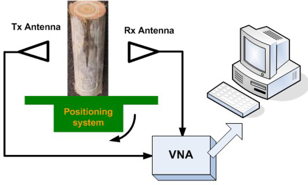
- Pastorino, M.; Salvade, A.; Monleone, R.; Bartesaghi, T.; Bozza, G.; Randazzo, A. Detection of Defects in Wood Slabs by Using a Microwave Imaging Technique. Proceedings of the IEEE Instrumentation and Measurement Technology Conference, (IMTC’07), Warsaw, Poland, 1–3 May 2007.
- Caorsi, S. Improved Microwave Imaging Procedure for Nondestructive Evaluation of Two Dimensional Structures; Technical Report; University of Pavia: Pavia, Italy, 2003. [Google Scholar]
- Caorsi, S.; Massa, A.; Pastorino, M.; Donelli, M. Improved microwave imaging procedure for nondestructive evaluations of two-dimensional structures. IEEE Trans. Antennas Propag 2004, 52, 1386–1397. [Google Scholar]
- Benedetti, M.; Donelli, M.; Martini, A.; Massa, A.; Rosani, A. An Innovative Microwave Imaging Technique for Non Destructive Evaluation: Applications to Civil Structures Monitoring and Biological Bodies Inspection; Technical Report; University of Trento: Trento, Italy, 2005. [Google Scholar]
- Benedetti, M.; Donelli, M.; Martini, A.; Pastorino, M.; Rosani, A.; Massa, A. An innovative microwave-imaging technique for nondestructive evaluation: Applications to civil structures monitoring and biological bodies inspection. IEEE Trans. Instrum. Meas 2006, 55, 1878–1884. [Google Scholar]
- Donelli, M.; Massa, A. Computational approach based on a particle swarm optimizer for microwave imaging of two-dimensional dielectric scatterers. IEEE Trans. Microwave Theory Tech 2005, 53, 1761–1776. [Google Scholar]
- Poli, L.; Rocca, P. Exploitation of TE-TM Scattering Data For Microwave Imaging Through the Multi-Scaling Reconstruction Strategy; Technical Report; University of Trento: Trento, Italy, 2011. [Google Scholar]
- Langenberg, K.; Mayer, K.; Marklein, R. Nondestructive testing of concrete with electromagnetic and elastic waves: Modeling and imaging. Cement Concr. Compos 2006, 28, 370–383. [Google Scholar]
- Zoughi, R.; Kharkovsky, S. Microwave and millimetre wave sensors for crack detection. Fatigue Fract. Eng. Mater. Struct 2008, 31, 695–713. [Google Scholar]
- Wu, Z.; McCann, H.; Davis, L.E.; Hu, J.; Fontes, A.; Xie, C.G. Microwave-tomographic system for oiland gas-multiphase-flow imaging. Meas. Sci. Technol 2009, 20, 104026. [Google Scholar]
- Zimdars, D.; Valdmanis, J.A.; White, J.S.; Stuk, G.; Williamson, S.; Winfree, W.P.; Madaras, E.I. Technology and applications of terahertz imaging nondestructive examination: Inspection of space shuttle sprayed on foam insulation. Rev. Quant. Nondestruct. Eval 2005, 24, 570–577. [Google Scholar]
- Hor, Y.L.; Federici, J.F.; Wample, R.L. Nondestructive evaluation of cork enclosures using terahertzmillimeter wave spectroscopy and imaging. Appl. Opt 2008, 47, 72–78. [Google Scholar]
- Kharkovsky, S.; Ghasr, M.T.; Zoughi, R. Near-field millimeter-wave imaging of exposed and covered fatigue cracks. IEEE Trans. Instrum. Meas 2009, 58, 2367–2370. [Google Scholar]
- Kemp, I.; Peterson, M.; Benton, C.; Petkie, D.T. Sub-mm wave imaging techniques for non-destructive aerospace materials evaluation. IEEE Aerosp. Electron. Syst. Mag 2010, 25, 17–19. [Google Scholar]
- Beckmann, J.; Richter, H.; Zscherpel, U.; Ewert, U.; Weinzierl, J.; Schmidt, L.P.; Rutz, F.; Koch, M.; Richter, H.; Hubers, H.W. Imaging Capability of Terahertz and Millimeter-Wave Instrumentations for NDT of Polymer Materials. Proceedings of the European Conference on NDT, (ECNDT’06), Berlin, Germany, September 2006.
- Zimdars, D.; White, J.S.; Stuk, G.; Chernovsky, A.; Fichter, G.; Williamson, S. Security and Non Destructive Evaluation Application of High Speed Time Domain Terahertz Imaging. Proceedings of theLasers and Electro-Optics, 2006 and 2006 Quantum Electronics and Laser Science Conference, (CLEO/QELS ’06), Long Beach, CA, USA, 21–26 May 2006.
- Oyama, Y.; Zhen, L.; Tanabe, T.; Kagaya, M. Sub-terahertz imaging of defects in building blocks. NDT&E Int 2009, 42, 28–33. [Google Scholar]
- Redo-Sanchez, A.; Kaur, G.; Zhang, X.C.; Buersgens, F.; Kersting, R. 2-D acoustic phase imaging with millimeter-wave radiation. IEEE Trans. Microwave Theory Tech 2009, 57, 589–593. [Google Scholar]
- Bogue, R. Terahertz imaging: A report on progress. Sens. Rev 2009, 29, 6–12. [Google Scholar]
- Jenks, W.G.; Sadeghi, S.S.H.; Wikswo, J.P., Jr. SQUIDs for nondestructive evaluation. J. Phys. D Appl. Phys 1997, 30, 293–323. [Google Scholar]
- Tralshawala, N.; Claycomb, J.R.; Miller, J.H. Practical SQUID instrument for nondestructive testing. Appl. Phys. Lett 1997, 71, 1753–1575. [Google Scholar]
- Krausea, H.J.; Kreutzbruck, M. Recent developments in SQUID NDE. Physica C: Superconductivity 2002, 368, 70–79. [Google Scholar]
- Xu, Y.; He, B. Magnetoacoustic tomography with magnetic induction (MAT-MI). Phys. Med. Biol 2005, 50, 5175–5187. [Google Scholar]
- Li, X.; Xu, Y.; He, B. Imaging electrical impedance from acoustic measurements by means of Magnetoacoustic Tomography with Magnetic Induction (MAT-MI). IEEE Trans. Biomed. Eng 2007, 54, 323–330. [Google Scholar]
- Redo-Sanchez, A.; Kaur, G.; Zhang, X.C.; Buersgens, F.; Kersting, R. 2-D acoustic phase imaging with millimeter-wave radiation. IEEE Trans. Microwave Theory Tech 2009, 57, 589–593. [Google Scholar]
- Deng, Y.; Golkowski, M. MIcrowave Induced Thermoacoustic Imaging: A Hybrid FDTD Model. Proceedings of The URSI National Conference, Boulder, USA, 5–10 January, 2011.
- Dorn, O.; Berte-Aguirey, H.; Beryman, J.; Papniolaou, G. A Nonlinear Inversion Method for 3D Eletromagnetic Imaging Using Adjoint Fields; Technical Report; Stanford University: Stanford, CA, USA, 1999. [Google Scholar]
- Dorn, O.; Miller, E.L.; Rappaport, C.M. A shape reconstruction method for electromagnetic tomography using adjoint fields and level sets. Inverse Probl 2000, 16, 1119–1156. [Google Scholar]
- Lionheart, W.R. Reconstruction Algorithms for Permittivity and Conductivity Imaging; Technical Report; The University of Manchester: Manchester, UK, 2001. [Google Scholar]
- Polydorides, N. Image Reconstruction Algorithms for Soft Field Tomography. Ph.D. Thesis,. University of Manchester, Manchester, UK, 2002. [Google Scholar]
- Mook, G.; Michel, F.; Simonin, J. Electromagnetic Imaging using Probe Arrays. Proceedings of the 10th International Conference of The Slovenian Society for Non-Destructive Testing, Ljubljana, Slovenia, 1–3 September 2009.
- Chaturvedi, P.; Plumb, R.G. Electromagnetic imaging of underground targets using constrained optimization. IEEE Trans. Geosci. Remote Sens 1995, 33, 551–561. [Google Scholar]
- Azaro, R.; Bozza, G.; Estatico, C.; Massa, A.; Pastorino, M.; Pregnolato, D.; Randazzo, A. New Results on Electromagnetic Imaging Based on the Inversion of Measured Scattered-Field Data. Proceedings of the Instrumentation and Measurement Technology Conference, (IMTC’05), Ottawa, ON, Canada, 16–19 May 2005.
- Dorn, O.; Lesselier, D. Level set methods for inverse scattering. Inverse Probl 2006, 22, R67–R131. [Google Scholar]
- Ammari, H.; Iakovleva, E.; Lesselier, D.; Perrusson, G. Music-type electromagnetic imaging of a collection of small three-dimensional inclusions. SIAM J. Sci. Comput 2007, 29, 674–709. [Google Scholar]
- Pastorino, M. Stochastic optimization methods applied to microwave imaging: A review. IEEE Trans. Antennas Propag 2007, 55, 538–548. [Google Scholar]
- Simm, A.; Abidin, I.Z.; Tian, G.Y.; Woo, W.L. Simulation and Visualisation for Electromagnetic Nondestructive Evaluation. Proceedings of the 14th International Conference Information Visualisation, London, UK, 26–29 July 2010.


© 2011 by the authors; licensee MDPI, Basel, Switzerland. This article is an open access article distributed under the terms and conditions of the Creative Commons Attribution license (http://creativecommons.org/licenses/by/3.0/).
Share and Cite
Deng, Y.; Liu, X. Electromagnetic Imaging Methods for Nondestructive Evaluation Applications. Sensors 2011, 11, 11774-11808. https://doi.org/10.3390/s111211774
Deng Y, Liu X. Electromagnetic Imaging Methods for Nondestructive Evaluation Applications. Sensors. 2011; 11(12):11774-11808. https://doi.org/10.3390/s111211774
Chicago/Turabian StyleDeng, Yiming, and Xin Liu. 2011. "Electromagnetic Imaging Methods for Nondestructive Evaluation Applications" Sensors 11, no. 12: 11774-11808. https://doi.org/10.3390/s111211774