Fuzzy Adaptive Interacting Multiple Model Nonlinear Filter for Integrated Navigation Sensor Fusion

Abstract
: In this paper, the application of the fuzzy interacting multiple model unscented Kalman filter (FUZZY-IMMUKF) approach to integrated navigation processing for the maneuvering vehicle is presented. The unscented Kalman filter (UKF) employs a set of sigma points through deterministic sampling, such that a linearization process is not necessary, and therefore the errors caused by linearization as in the traditional extended Kalman filter (EKF) can be avoided. The nonlinear filters naturally suffer, to some extent, the same problem as the EKF for which the uncertainty of the process noise and measurement noise will degrade the performance. As a structural adaptation (model switching) mechanism, the interacting multiple model (IMM), which describes a set of switching models, can be utilized for determining the adequate value of process noise covariance. The fuzzy logic adaptive system (FLAS) is employed to determine the lower and upper bounds of the system noise through the fuzzy inference system (FIS). The resulting sensor fusion strategy can efficiently deal with the nonlinear problem for the vehicle navigation. The proposed FUZZY-IMMUKF algorithm shows remarkable improvement in the navigation estimation accuracy as compared to the relatively conventional approaches such as the UKF and IMMUKF.1. Introduction
A navigation filter is commonly designed by use of an extended Kalman filter (EKF) [1–3] to estimate the vehicle state variables and suppress the navigation measurement noise. Although it has been shown to be a minimum mean square error estimator, the fact that EKF highly depends on a predefined dynamics model forms a major drawback. For achieving good filtering results, the designers are required to have the complete a priori knowledge on both the dynamic process and measurement models, in addition to the assumption that both the process and measurement are corrupted by zero-mean Gaussian white sequences.
As a deterministic sampling approach, the unscented Kalman filter (UKF) [4–9] was first proposed by Julier, et al. [4] to address nonlinear state estimation in the context of control theory. The UKF is a nonlinear, distribution approximation method, which uses a finite number of carefully chosen sigma points to propagate the probability of state distribution through the nonlinear dynamics of system so as to completely capture the true mean and covariance of the Gaussian random variable (GRV) with a minimal set of samples. The UKF made a Gaussian approximation with a limited number sigma points by using the Unscented Transform (UT). The basic premise behind the UKF is it is easier to approximate a Gaussian distribution than it is to approximate an arbitrary nonlinear function. When the sample points are propagated through the true nonlinear system, the posterior mean and covariance can be captured accurately to the second order of Taylor series expansion for any nonlinear system. One of the remarkable merits is that the overall computational complexity of the UKF is the same as that of the EKF [8].
A high gain (high bandwidth) filter is needed to respond fast enough to the platform maneuvers while a low gain filter is necessary to reduce the estimation errors during the uniform motion periods. Under various circumstances where there are uncertainties in the system model and noise description, and the assumptions on the statistics of disturbances are violated due to the fact that in a number of practical situations, the availability of a precisely known model is unrealistic. One way to take them into account is to consider a nominal model affected by uncertainty. An a parametric adaptation approach, the adaptive Kalman filter (AKF) algorithm has been one of the strategies considered for estimating the state vector to prevent divergence problem due to modeling errors [9–11]. Many efforts have been made to improve the estimation of the covariance matrices based on the innovation-based estimation approach, resulting in the innovation adaptive estimation (IAE) [2,10,11]. Two popular types of the adaptive Kalman filter algorithms include the innovation-based adaptive estimation (IAE) approach [10,11] and the adaptive fading memory filter approach, which is a type of covariance scaling method. One of the adaptive fading memory filters is called the strong tracking Kalman filter [9], where the strong tracking algorithm (STA) involves a nonlinear smoother algorithm that employs suboptimal multiple fading factors.
The other major approach that has been proposed for AKF is the multiple model adaptive estimate (MMAE). An a structural adaptation approach, the interacting multiple model (IMM) algorithm [3,12,13] has the configuration that runs in parallel several model-matched state estimation filters, which exchange information (interact) at each sampling time. The IMM approach is based on filter structural adaptation (model switching). Based on a soft-switching framework, the IMM algorithm allows the possibility of using highly dynamic models just when required, diminishing unrealistic noise considerations in non-maneuvering situations of the system. The use of an IMM allows exploiting the benefits of high dynamic models in the problem of vehicle navigation. The IMM estimator obtains its estimate as a weighted sum of the individual estimates from a number of parallel filters matched to different motion modes of the platform. The objective is to design the nonlinear filter in an IMM algorithm suitable for high dynamic or curvilinear motions to navigate a maneuvering vehicle. Selected results presented in this paper confirm the improvements.
The IMM algorithm has been originally applied to target tracking [14–17], and recently extended to Global Positioning System (GPS) navigation [18,19], and integrated navigation designs [20–23]. A model probability evaluator calculates the current probability of the vehicle being in each of the possible modes. A global estimate of the vehicle’s state is computed using the latest mode probabilities. This algorithm carries out a soft-switching between the various modes by adjusting the probabilities of each mode, which are used as weightings in the combined global state estimate. The covariance matrix associated with this combined estimate takes into account the covariances of the mode-conditioned estimates as well as the differences between these estimates.
The UKF naturally suffers the same problem as the EKF. The uncertainty of the process noise and measurement noise will degrade the performance of the UKF. An adaptive mechanism which dynamically identifies uncertainties or modeling errors can be adopted. To deal with the noise uncertainty and system nonlinearity simultaneously, the IMMUKF can be introduced [24,25]. In the approach, these multiple models are developed to describe various dynamic behaviors. In each model an UKF is running, and the IMM algorithm makes uses of model probabilities to weight the inputs and output of a bank of parallel filters at each time instant. The fuzzy logic reasoning system is based on the Takagi-Sugeno (T-S) model. The fuzzy reasoning system is constructed for obtaining the suitable process noise according to the time-varying change in dynamics. By monitoring the innovation information, the Fuzzy logic adaptive system (FLAS) is employed for dynamically on-line determining better lower and upper bounds of the process noise covariance according to the innovation information, and therefore improves the estimation performance.
The synergy of Global Positioning System (GPS) and inertial navigation system (INS) has been widely explored due to their complementary operational characteristics [1,26]. The GPS/INS integrated navigation system, typically carried out through the EKF and UKF, is the adequate solution to provide a navigation system that has the superior performance in comparison with either the GPS or INS stand-alone system. The example on the tightly-coupled GPS/INS integrated navigation processing based on the FUZZY-IMMUKF will be presented. The performance comparison will be demonstrated by using the proposed FUZZY-IMMUKF method as compared to the relatively conventional UKF and IMMUKF approaches.
The remainder of this paper is organized as follows. In Section 2, the preliminary background on the interacting multiple model unscented Kalman filter for the navigation processing is discussed. The proposed sensor fusion strategy is introduced in Section 3. In Section 4, the navigation integration processing and performance evaluation are carried out to evaluate the performance comparison will be demonstrated using the proposed FUZZY-IMMUKF method as compared to the relatively conventional UKF and IMMUKF approaches. Conclusions are given in Section 5.
2. The Interacting Multiple Model Unscented Kalman Filter
The unscented Kalman filtering deals with the case governed by the nonlinear stochastic difference equations:
The IMM approach takes into account a set of models to represent the system behaviour patterns or system model. The estimator carries out a ‘soft switching’ among various models by the model probability. The overall estimates is obtained by a combination of the estimates from the filters running in parallel based on the individual models that match the system modes. The measurements could be obtained from one or more sensors, and the model-matched filters could be linear or nonlinear. The algorithm of IMM-nonlinear filters is introduced to deal with the noise uncertainty and system nonlinearity simultaneously.
Let a general system for multiple models in discrete time be described by:
Instead of linearizing using the Jacobian matrices as in the EKF and achieving first-order accuracy, the UKF uses a deterministic sampling approach to capture the mean and covariance estimates with a minimal set of sample points. The UKF was proposed to address nonlinear state estimation in the context of control theory. When the sample points are propagated through the true nonlinear system, the posterior mean and covariance can be captured accurately to the 3rd order of Taylor series expansion for any nonlinear system. One of the remarkable merits is that the overall computational complexity of the UKF is the same as that of the EKF [8].
The first step in the UKF is to sample the prior state distribution, i.e., generate the sigma points through the UT, which is a method for calculating the statistics of a random variable which undergoes a nonlinear transformation. The basic premise is that to approximate a probability distribution is easier than to approximate an arbitrary nonlinear transformation. The samples are propagated through true nonlinear equations, and the linearization of the model is not required.
Suppose the mean x̄ and covariance P of vector x are known, a set of deterministic vector called sigma points can then be found. The ensemble mean and covariance of the sigma points are equal to x̄ and P. The nonlinear function y = f (x) is applied to each deterministic vector to obtain transformed vectors. The ensemble mean and covariance of the transformed vectors will give a good estimate of the true mean and covariance of y, which is the key to the unscented transformation. The UKF approach estimates are expected to be closer to the true values than the EKF approach.
The sigma vectors are propagated through the nonlinear function to yield a set of transformed sigma points:
The mean and covariance of yi are approximated by a weighted average mean and covariance of the transformed sigma points as follows:
As compared to the EKF’s linear approximation, the unscented transformation is accurate to the second order for any nonlinear function. The UKF algorithm is summarized in Appendix. Incorporation of the STA (also provided in Appendix) into the UKF results in the strong tracking unscented Kalman filter (STUKF).
The IMMUKF algorithm uses model (Markov chain state) probabilities to weight the input and output of a bank of parallel UKFs at each time instant. The approach takes into account a set of models to represent the system behavior patterns or system model. The overall estimates is obtained by a combination of the estimates from the filters running in parallel based on the individual models that match the system modes. An IMM cycle consists of four major stages: interaction (mixing), filtering, model probability calculation, and estimate combination, as described in the following subsections.
2.1. Model Interaction/Mixing
For given states with corresponding covariances and mixing probabilities for every model, the initial condition for the model j is:
The covariance corresponding to the above is:
The model transition probabilities, which are related to Markov chain, are defined as:
2.2. Model Individual Filtering
- Step 1 in UKF loop. The unscented transform creates 2n+ 1 sigma vectors X (a capital letter) and weighted points W. For state estimation at instant k − 1, sigma points are generated according to:
where is the i th row (or column) of the matrix square root. can be obtained from the lower-triangular matrix of the Cholesky factorization; λ = α2(n + k) − n is a scaling parameter used to control the covariance matrix; α determines the spread of the sigma points and is usually set to a small positive (e.g., 1e − 4 ≤ α ≤ 1); k is a secondly scaling parameter (usually set as 0); β is used to incorporate prior knowledge of the distribution of x̄ (when x is normally distributed, β = 2 is an optimal value); is the weight for the mean associated with the i th point; and is the weight for the covariance associated with the i th point:- Step 2 in UKF loop. Time update (prediction steps):
- Step 3 in UKF loop. Measurement update (correction steps):
The samples are propagated through true nonlinear equations; the linearization is unnecessary (Calculation of the Jacobian matrix is not required).
2.3. Model Probabilities Update
The model probability is updated according to the model likelihood and model transition probability governed by the finite-state Markov chain:
2.4. Combination of State Estimation and Covariance Combination
The model-individual estimates and covariances are combined to an overall state and covariance:
3. The Proposed Fuzzy Adaptive Filter Strategy
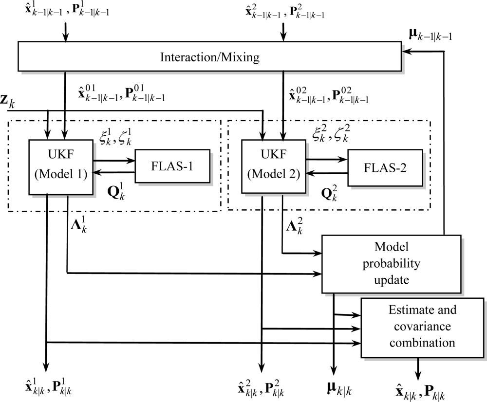
Figure 1 shows the block diagram for implementation of the proposed FUZZY-IMMUKF algorithm. The block on the right hand side, indicated by the dashed-line, is the fuzzy logic adaptive system (FLAS) for determining the value of process noise covariance. The rest represents the IMMUKF loop.
3.1. The Fuzzy Logic Adaptive System (FLAS)
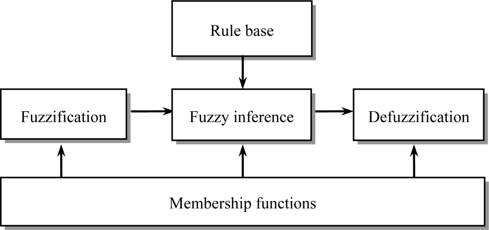
Fuzzy logic was first developed by Zadeh in the mid-1960s for representing uncertain and imprecise knowledge. It provides an approximate but effective means of describing the behavior of systems that are too complex, ill-defined, or not easily analyzed mathematically. A typical fuzzy system consists of three components, that is, fuzzification, fuzzy reasoning (fuzzy inference), and fuzzy defuzzification, as shown in Figure 2. The fuzzification process converts a crisp input value to a fuzzy value, the fuzzy inference is responsible for drawing calculations from the knowledge base, and the fuzzy defuzzification process converts the fuzzy actions into a crisp action.
The fuzzification modules: (1) transforms the error signal into a normalized fuzzy subset consisting of a subset for the range of the input values and a normalized membership function describing the degree of confidence of the input belonging to this range; (2) selects reasonable and good, ideally optimal, membership functions under certain convenient criteria meaningful to the application. The characteristics of the fuzzy adaptive system depend on the fuzzy rules and the effectiveness of the rules directly influences its performance. To obtain the best deterministic output from a fuzzy output subset, a procedure for its interpretation, known as defuzzification should be considered. The defuzzification is used to provide the deterministic values of a membership function for the output. Using fuzzy logic to infer the consequent of a set of fuzzy production rules invariably leads to fuzzy output subsets.
The fuzzy modeling is the method of describing the characteristics of a system using fuzzy inference rules. In this paper, a Takagi-Sugeno (T-S) fuzzy system is used to detect the divergence of EKF and adapt the filter. Takagi and Sugeno proposed a fuzzy modeling approach to model nonlinear systems.
The output is the weighted average of the yk:
3.2. The Fuzzy Adaptive System Based on Unscented Kalman Filter
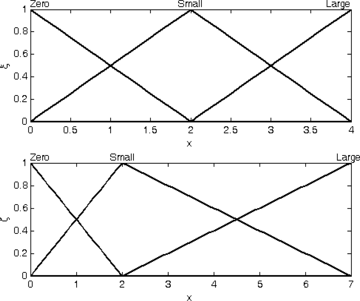
The degree of divergence (DOD) parameters for identifying the degree of change in vehicle dynamics needs to be defined. Examples for possible approaches are given as follows. The innovation information at the present epoch is employed for timely reflect the change in vehicle dynamics. The DOD parameter ξ can be defined as the trace of innovation covariance matrix at present epoch (i.e., the window size is one) divided by the number of satellites employed for navigation processing:
In the FLAS, the DOD parameters are employed as the inputs for the fuzzy inference engines. By monitoring the DOD parameters, the FLAS is able to on-line determine better lower and upper bounds of the process noise covariance according to the innovation information, and therefore improves the estimation performance. The flow chart of the FLAS-UKF algorithm is shown in Figure 3.
5. Conclusions
The classical unscented Kalman filter does not possess the capability to monitor parameter changes due to changes in vehicle dynamics. An interacting multiple-model based method is suggested to improve the unscented Kalman filter for better navigation data fusion. The resulting IMMUKF ensures better description on the vehicle dynamics and exhibits superior navigation accuracy when compared with the classical UKF algorithm. This paper has presented a fuzzy interacting multiple model unscented Kalman filter for GPS/INS navigation processing to prevent the divergence problem in high dynamic environments.
The fuzzy system is employed for dynamically adjusting the lower and upper bounds of the process noise covariance, which will be used in each of the parallel filters in the IMM architecture by monitoring the innovation information so as to provide further improvement in estimation accuracy. Through the proposed approach, lower order of filter model can be utilized and, therefore, less computational effort will be sufficient without compromising estimation accuracy significantly. When a designer does not have sufficient information to develop the complete filter models or when the filter parameters are slowly changing with time, the fuzzy system can be employed to enhance the IMMUKF performance. These performance comparisons of UKF, IMMUKF and FUZZY-IMMUKF have been conducted and the proposed FUZZY-IMMUKF algorithm has demonstrated very promising results in navigational accuracy. Future research can be conducted to undertake the implementation of the following issues.
The current work essentially shows the feasibility of the approach. Evaluation of the proposed approach on a real system with better design of the fuzzy logic might be considered in the near future. Other artificial intelligence such as neural work may also be incorporated for better tuning. Furthermore, the GPS RAIM (Receiver Autonomous Integrity Monitoring) in civil aviation might also be considered as one of the potential applications.
Acknowledgments
Funding for this work was provided by the National Science Council of the Republic of China under grant number NSC 97-2221-E-019-012 and NSC 98-2221-E-019-MY3.
References
- Brown, R.G.; Hwang, P.Y.C. Introduction to Random Signals and Applied Kalman Filtering; John Wiley & Sons: New York, NY, USA, 1997. [Google Scholar]
- Gelb, A. Applied Optimal Estimation; MIT Press: Cambridge, MA, USA, 1974. [Google Scholar]
- Li, X.R.; Bar-Shalom, Y. Estimation with Applications to Tracking and Navigation; John Wiley & Sons: New York, NY, USA, 1993. [Google Scholar]
- Julier, S.J.; Uhlmann, J.K.; Durrant-whyte, H.F. A new approach for filtering nonlinear system. Proceedings of the American Control Conference, Seattle, WA, USA, 21–23 June 1995; pp. 1628–1632.
- Julier, S.J.; Uhlmann, J.K.; Durrant-Whyte, H.F. A new method for the nonlinear transformation of means and covariances in filters and estimators. IEEE Trans. Automat. Contr 2000, 5, 477–482. [Google Scholar]
- Julier, S.J. The scaled unscented transformation. Proceedings of the American Control Conference, Anchorage, AK, USA, May 2002; pp. 4555–4559.
- Julier, S.J.; Uhlmann, J.K. Reduced sigma point filters for the propagation of means and covariances through nonlinear transformations. Proceedings of the American Control Conference, Anchorage, AK, USA, May 2002; pp. 887–892.
- Wan, E.A.; van der Merwe, R. The unscented Kalman filter for nonlinear estimation. Proceedings of Adaptive Systems for Signal Processing, Communication and Control (AS-SPCC) Symposium, Alberta, Canada, October 2000; pp. 153–156.
- Jwo, D.J.; Lai, S.Y. Navigation integration using the fuzzy strong tracking unscented Kalman filter. J. Navig 2009, 62, 303–322. [Google Scholar]
- Mohamed, A.H.; Schwarz, K.P. Adaptive Kalman filtering for INS/GPS. J. Geodesy 1999, 73, 193–203. [Google Scholar]
- Hide, C; Moore, T.; Smith, M. Adaptive Kalman filtering for low cost INS/GPS. J. Navig 2003, 56, 143–152. [Google Scholar]
- Li, X.R.; Bar-Shalom, Y. Performance prediction of the interacting multiple model algorithm. IEEE Trans. Aerosp. Electron. Syst 1993, 29, 755–771. [Google Scholar]
- Kim, Y.S.; Hong, K.S. An IMM algorithm for tracking maneuvering vehicles in an adaptive cruise control environment. Int. J. Control Autom. Syst 2004, 2, 310–318. [Google Scholar]
- Lee, B.J.; Park, J.B.; Lee, H.J.; Joo, Y.H. Fuzzy-logic-based IMM algorithm for tracking a manoeuvring target. IEE Proc.-Radar Sonar Navig 2005, 152, 16–22. [Google Scholar]
- Li, X.R.; Bar-Shalom, Y. Design of an interacting multiple model algorithm for air traffic control tracking. IEEE Trans. Control Syst. Technol 1993, 1, 186–194. [Google Scholar]
- Zhou, Y.; Xu, J.; Jing, Y.; Dimirovski, G.M. Extended target tracking using an IMM based nonlinear Kalman filters. Proceeding of the 2010 American Control Conference, Baltimore, MD, USA, 30 June–2 July 2010; pp. 6876–6881.
- Chen, G.; Harigae, M. Using IMM adaptive estimator in GPS positioning. Proceeding of the 40th SICE Annual Conference, Tampa, FL, USA, July 2001; pp. 78–83.
- Lin, X.; Kirubarajan, T.; Bar-Shalom, Y.; Li, X. Enhanced accuracy GPS navigation using the interacting multiple model estimator. Proceedings of IEEE Aerospace Conference, Big Sky, MT, USA, March 2001; 4, pp. 1911–1923.
- Zang, R.C.; Cui, P.Y. An innovation filtering multiple model algorithm for integrated navigation system. Proceedings of the First International Conference on Innovative Computing, Information and Control, Beijing, China, 30 August–1 September 2006; pp. 394–397.
- Toledo-Moreo, R.; Zamora-Izquierdo, M.A.; Ubeda-Miarro, B.; Gomez-Skarmeta, A.F. High-integrity IMM-EKF-based road vehicle navigation with low-cost GPS/SBAS/INS. IEEE Trans. Intell. Transp. Syst 2007, 8, 491–511. [Google Scholar]
- Toledo-Moreo, R.; Zamora-Izquierdo, M.A. IMM-based lane-change prediction in highways with low-cost GPS/INS. IEEE Trans. Intell. Transp. Syst 2009, 10, 180–185. [Google Scholar]
- Crassidis, J.L. Sigma-point Kalman filtering for integrated GPS and inertial navigation. IEEE Trans. Aerosp. Electron. Syst 2006, 42, 750–756. [Google Scholar]
- Li, Y.; Wang, J.; Rizos, C.; Mumford, P.; Ding, W. Low-cost tightly coupled GPS/INS integration based on a nonlinear Kalman filter design. Proceedings of the U.S. Institute of Navigation National Technical Meeting, Monterey, CA, USA, 18–20 January 2006; pp. 958–966.
- Qian, H.; An, D.; Xia, Q. IMM-UKF based land-vehicle navigation with low-cost GPS/INS. Proceedings of the 2010 IEEE International Conference on Information and Automation, Harbin, China, 20–23 June 2010; pp. 2031–2035.
- Cork, L.; Walker, R. Sensor fault detection for UAVs using a nonlinear dynamic model and the IMM-UKF algorithm. Proceedigns of the 2007 Information, Decision and Control, Adelaide, Australia, 12–14 February 2007; pp. 230–235.
- Farrell, J.; Barth, M. The Global Positioning System and Inertial Navigation; McGraw-Hill Professional: Dubuque, IA, USA, 1999. [Google Scholar]
Appendix
A. The Unscented Kalman Filter
Consider an n dimensional random variable x, having the mean x̂ and covariance P, and suppose that it propagates through an arbitrary nonlinear function f. The unscented transform creates 2n + 1 sigma vectors X (a capital letter) and weighted points W, given by:
The implementation algorithm of UKF is summarized as follows:
The transformed set is given by instantiating each point through the process model:
Predicted mean:
Predicted covariance:
Instantiate each of the prediction points through observation model:
Predicted observation:
Innovation covariance:
Cross covariance:
Performing update:
B. The Strong Tracking Algorithm
Based on the idea as in the AKF, the synthesis of UKF and strong tracking filter leads to the strong tracking unscented Kalman filter (STUKF). The suboptimal fading factors are introduced into the nonlinear smoother algorithm:
The covariance matrix needs to be updated the following way. The new needs to be modified and can be obtained by multiplying Equation (42) by the factor Sk:
Similarly, the covariance matrix Pzz and Pxz, as represented by Equations (43) and (44), also respectively, can be modified and rewritten as:


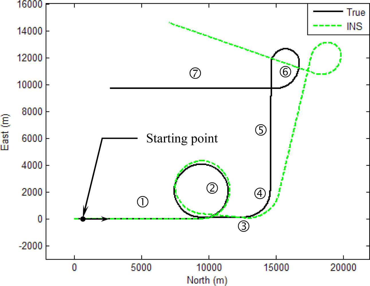
| Segment number | Time interval (sec) | Motion |
|---|---|---|
| 1 | [0–300] | Constant velocity straight line |
| 2 | [301–700] | Circular motion (counter-clockwise) |
| 3 | [701–800] | Constant velocity straight line |
| 4 | [801–900] | Counter-clockwise turn |
| 5 | [901–1,200] | Constant velocity straight line |
| 6 | [1,201–1,400] | Clockwise turn |
| 7 | [1,401–1,800] | Constant velocity straight line |
| East | North | |
|---|---|---|
| UKF | 7.9530 | 6.3195 |
| IMMUKF | 2.9967 | 2.3021 |
| FUZZY-IMMUKF | 1.0184 | 0.7286 |
© 2011 by the authors; licensee MDPI, Basel, Switzerland. This article is an open access article distributed under the terms and conditions of the Creative Commons Attribution license (http://creativecommons.org/licenses/by/3.0/).
Share and Cite
Tseng, C.-H.; Chang, C.-W.; Jwo, D.-J. Fuzzy Adaptive Interacting Multiple Model Nonlinear Filter for Integrated Navigation Sensor Fusion. Sensors 2011, 11, 2090-2111. https://doi.org/10.3390/s110202090
Tseng C-H, Chang C-W, Jwo D-J. Fuzzy Adaptive Interacting Multiple Model Nonlinear Filter for Integrated Navigation Sensor Fusion. Sensors. 2011; 11(2):2090-2111. https://doi.org/10.3390/s110202090
Chicago/Turabian StyleTseng, Chien-Hao, Chih-Wen Chang, and Dah-Jing Jwo. 2011. "Fuzzy Adaptive Interacting Multiple Model Nonlinear Filter for Integrated Navigation Sensor Fusion" Sensors 11, no. 2: 2090-2111. https://doi.org/10.3390/s110202090