Development of a Stereo Vision Measurement System for a 3D Three-Axial Pneumatic Parallel Mechanism Robot Arm

Abstract
: In this paper, a stereo vision 3D position measurement system for a three-axial pneumatic parallel mechanism robot arm is presented. The stereo vision 3D position measurement system aims to measure the 3D trajectories of the end-effector of the robot arm. To track the end-effector of the robot arm, the circle detection algorithm is used to detect the desired target and the SAD algorithm is used to track the moving target and to search the corresponding target location along the conjugate epipolar line in the stereo pair. After camera calibration, both intrinsic and extrinsic parameters of the stereo rig can be obtained, so images can be rectified according to the camera parameters. Thus, through the epipolar rectification, the stereo matching process is reduced to a horizontal search along the conjugate epipolar line. Finally, 3D trajectories of the end-effector are computed by stereo triangulation. The experimental results show that the stereo vision 3D position measurement system proposed in this paper can successfully track and measure the fifth-order polynomial trajectory and sinusoidal trajectory of the end-effector of the three- axial pneumatic parallel mechanism robot arm.1. Introduction
Many manufacturing processes use robots to perform various tasks, include welding, assembling, pick and place, and defect inspection. All these tasks require knowledge of the relative location between the robot’s end-effector and the desired target. The best-known technique to determine three-dimensional location information is based on stereo vision. Stereo vision systems often consist of two or multiple imaging devices along with a PC or other microprocessors. Due to the advantages of cost, easy maintenance, reliability, and non-contact measurement, stereo vision has become a popular research topic and been applied in industrial automation, autonomous vehicles, augmented reality, medical, and transportation [1–4].
A three-axial pneumatic parallel mechanism robot arm developed by NTU-AFPC Lab [5] was the test rig in this study. Its end-effector is able to follow the desired trajectories by controlling the positions of three rod-less pneumatic cylinders using nonlinear servo control. However, the kinematic model of the test rig has many different solutions so the real trajectories of the end-effector cannot be known only by the measured position of the three pneumatic actuators. To solve this problem, a common method is to use angular sensors for measuring angular displacements of each joint, and the trajectory of the end-effector can be calculated and estimated by the robot forward kinematics. Compared the joint angle measuring method with the stereo vision method, the stereo vision method has the advantages of involving non-contact sensing and providing direct measurements. Besides, it’s very difficult to fit angular sensors at the joints of parallel mechanism of the robot due to the restrictions of the mechanism used in this study.
To reconstruct a 3D space by stereo images using binocular cues, the disparities of the corresponding points in stereo pairs have to be known. Therefore, solving the stereo correspondence problem has been the most important stage on the 3D reconstruction. Some published studies [6–9] have attempted to solve the stereo correspondence problem. The most popular and well-known method is to use epipolar constraints [10] to reduce the stereo matching region from an area to a straight line.
For an uncalibrated stereo rig (i.e., both intrinsic and extrinsic parameters are unknown) [11–13], the fundamental matrix F often needs to be computed to express epipolar constraints on uncalibrated stereo pairs. In contrast, a calibrated stereo rig with known intrinsic and extrinsic parameters can use so-called epipolar rectification [14,15] to transform each corresponding stereo pair for making the epipolar lines parallel and at the same horizontal rows, which greatly reduces the stereo matching region to a horizontal row. In this paper, the epipolar rectification algorithm [15] is adapted, which is a compact and clear stereo rectification algorithm and can provide MATLAB code for research reference. Since the algorithm assumes that the stereo rig is calibrated, camera calibration needs to be performed first.
The camera calibration procedure in this paper was accomplished using the Camera Calibration Toolbox of MATLAB [16] developed by Bouquet. Bouquet’s main initialization phase of camera calibration inspires by Zhang [17] that uses a chessboard as calibration pattern to obtain both intrinsic and extrinsic camera parameters, and Bouquet’s intrinsic camera model inspired by Heikkilä and Silvén [18] which includes two extra distortion coefficients of Zhang’s intrinsic camera model to get more precise stereo rectification. After stereo rectification is done, the correspondence problem of desired target is solved.
The Circle Hough Transform (CHT) [19] is one of the best known methods which aims to detect lines or circles in an image. The algorithm transforms each edge point in edge map to parameter space and plots histogram of parameter space in an accumulator space as output image in which the highest-frequency accumulator cell (i.e., pixel with the highest gray value) is the outcome. If circle radii are unknown, the parameter space is a three-dimensional space, and that requires a large amount of computing power for the algorithm, which is the major drawback for real-time application. Kimme et al. [20] first suggested that using edge direction can reduce the computational requirements of the CHT to only an arc to be plotted in the accumulator space. Minor and Sklansky [21], and Faez et al. [22] then proposed that plotting a line in the edge direction has the advantage of reducing parameter space to a two dimensional space. Scaramuzza et al. [23] developed a new algorithm which rejects non-arc segments (e.g., isolated points, noises, angular points, and straight segments) and plots lines in the direction of arc concavity. The algorithm gives more precise approximation for circle location.
There are two major procedures in stereo vision tracking, including motion tracking and stereo matching [24]. The location of the desired target in the reference image (e.g., the left image) is tracked by using the motion tracking algorithm, and the stereo matching algorithm is then matching the correspondence location of the desired target in the other image (e.g., the right image).
Motion tracking involves two types of algorithms: feature-based tracking algorithm [25,26] and region-based tracking algorithm [27–29]. The feature-based tracking algorithm tracks partial features of the target. The canny edge detector [30] is often used for extracting edge features of the target, and point feature of the target’s corner is extracted by the SUSAN corner detector [31]. Region-based tracking algorithm uses the template/block determined by user selection or image recognition to track the target. Once the template/block is decided, the algorithm starts to compute the correlation between the template/block and the designated region in the current frame. The most common used correlation criteria are the sum of absolute differences (SAD) and the sum of squared differences (SSD). References [28,29] suggested the template update strategies that solve the “drifting” problem caused by environmental influence (e.g., light conditions or object occlusion) during motion tracking.
The developed stereo matching methods can roughly be divided into two categories: local methods and global methods [32]. Although global methods, such as those using dynamic programming [33], can be less sensitive to local ambiguous regions (e.g., occlusion regions or regions with uniform texture in an image) than those using the local method, the global methods require more computing cost [34]. Block matching [35] is the best known method among the local methods because of its efficiency and simplicity in implementation. In the block matching, the reference block determined in moving tracking is used to search stereo corresponding by using matching criteria such as SSD or SAD. Once the stereo matching is made, each corresponding locations of the target in the stereo images are found, that is, the disparity of the target’s location is known. Therefore, the depth information of the target can be calculated by triangulation.
This paper aims to develop a stereo vision system that is considered as a sensor to measure 3D space trajectories of the end-effector of the three-axial pneumatic parallel mechanism robot arm in real-time. Thus, the real-time stereo tracking is required to ensure that the stereo measurement process and the end-effector’s motion are as synchronized as much as possible. The Multimedia Extension (MMX) technology [6] is utilized in this paper to minimize the computational cost of the stereo tracking process. In addition, the stereo depth estimation will be calibrated by the linear encoder measuring results on a straight-line moving pneumatic cylinder. Therefore, the correctness of stereo vision system can be known. For that, a test rig is set up for realizing the developed strategies of the stereo vision which is used to measure the end-effector of the three-axial pneumatic parallel mechanism robot arm.
2. System Setup
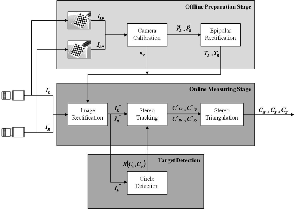
The system setup combines the stereo vision measuring method with the three-axial pneumatic parallel mechanism robot arm for measuring the 3D trajectories of the end-effector. Based on the structure design, the position of the end-effector of the three-axial pneumatic parallel mechanism robot arm is very difficult to measure directly in the practical experiment. It can be calculated via the position sensors of the three linear actuators by means of the kinematics. However, there are many different solutions for the kinematics of the end-effector of the three-axial pneumatic parallel mechanism robot arm, so the accurate xyz coordinates of the end-effector are difficult to solve. Thus, this paper proposes the stereo vision measuring method to measure the absolute xyz coordinates of the end-effector after the image coordinate calibration. In this paper, the stereo vision measurement system can be divided into two parts: the offline preparation stage and the online measuring stage, as shown in Figure 1.
The offline preparation stage of the system includes camera calibration and calculation of transformation matrices for epipolar rectification, and a series of calibration patterns must be taken for this stage. After each camera of the stereo rig is calibrated independently, both projection matrices and radial distortion coefficients of the left and right cameras are used to compute the transformation matrices and to rectify the distorted images.
In the online measuring stage, the transformation matrices and the radial distortion coefficients calculated at the offline preparation part are imported for the image rectification. In the first place, the desired target is detected in the rectified left image by means of circle detection, and the reference block for stereo tracking is defined.
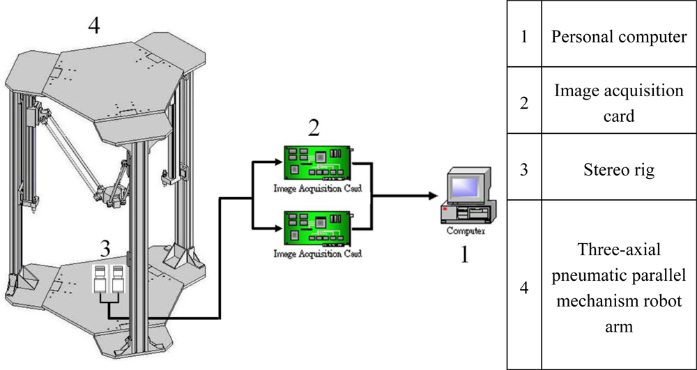
Once all requirements mentioned above are computed, the real-time 3D measurement can be executed. The target locations in both left and right image are tracked by stereo tracking so as to compute the estimated 3D world coordinates of the target through stereo triangulation. Figure 2 shows the system scheme of the stereo vision measurement system.
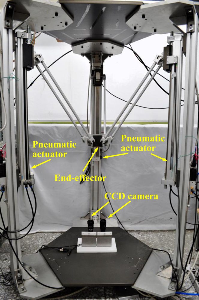
The stereo rig in this study, as shown in Figure 3, is composed of two identical CCD cameras which are equipped with camera lenses, and the baseline distance is approximately 7 cm. Figure 3 also shows the three-axial pneumatic parallel mechanism robot arm developed by the NTU-AFPC lab [5]. The end-effector is the desired target of the stereo vision measurement system.
Based on image quality and anti-noise performance, the CCD image sensor is better than the CMOS image sensor, thus, the CCD camera is selected in this paper [36]. A camera manufactured by TOSHIBA TELI, model CS8550Di, which supports progressive area scan and interlaced area scan, is utilized in this paper For the real-time application aspect, the progressive area scan is used in this paper. The detailed specificationd of the camera are shown in Table 1.
An analog CCD camera has analog signals, so it needs an image acquisition device to digitalize the analog signals for further processing or analyzing on a PC or other processors. The image acquisition card developed by National Instruments, model IMAQ PCI-1410 is chosen in this paper. It has 16 MB of onboard SDRAM used to temporarily store the image being transferred to the PCI bus, and three independent onboard DMA (Direct memory access) controllers for improving its performance. The intensity resolution can reach 10 bit/pixel, and 8-bit pixel format is supported on software programming. Table 1 shows its detailed specifications.
3. Image Rectification
Given a pair of stereo images, the problem of finding pixels or objects in one image which can be identified as the same pixels or objects in another image is called the correspondence problem. Solving the correspondence problem is difficult, due to problems such as object occlusion, lens distortion, aperture problem, and homogeneous regions in the stereo pair [39]. These problems make the correspondence problem difficult and complex. To make it easier, the image rectification is introduced.
Rectifying stereo images involves finding a transformation for each image plane such that pairs of conjugate epipolar lines become collinear and parallel to one of the image horizontal axes. Because the search of corresponding points becomes only along the horizontal lines of rectified images, the stereo rectification makes the correspondence problem easier. In the following sections, the stereo-pair image rectification methods applied in this paper will be introduced.
3.1. Camera Model
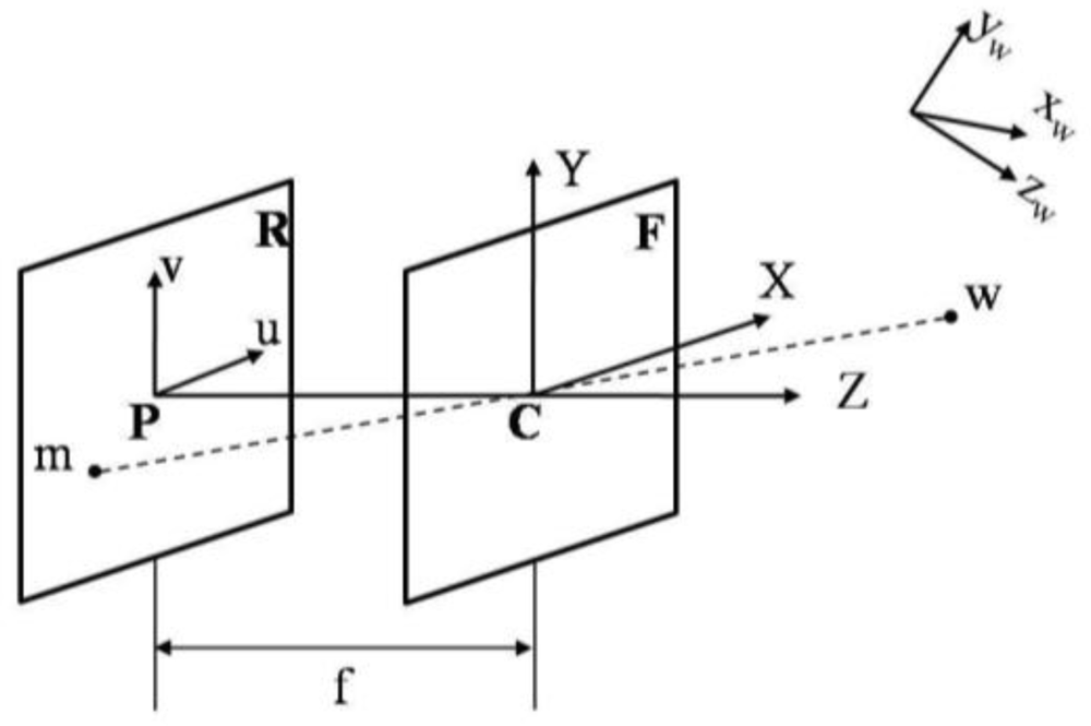
To rectify the stereo images, the knowledge of camera model and its parameters are important. Figure 4 depicts the pinhole camera model, which is the simplest camera model that describes the mathematical relationship between the 3D world coordinates and the image plane coordinates.
R is the image plane (or retinal plane) centered on the principle point P; F is the focal plane centered on the optical center C. Both planes are parallel to the focal length f. The straight line passing through the principle point P and the optical center C is called the optical axis.
A three-dimensional point is defined to be the homogeneous coordinates in the world reference frame (fixed arbitrarily) and is defined to be the homogeneous coordinates in the image frame {u v} (pixels) where s is the scale factor. Assume that a homogeneous transformation matrix P̃ exists and is given by:
In Equation (1), the homogeneous transformation matrix P̃ is also called the perspective projection matrix (PPM), which can be considered as the combination of transformations: the extrinsic parameters Te and the intrinsic parameters Ti. Therefore, the homogeneous coordinates in the image frame m̃ can be written as:
The extrinsic parameters Te define the position and the orientation of the camera reference frame with respect to the world reference frame by a rotation R and a translation t:
The intrinsic parameters Ti are the optical characteristics and the internal geometric of the camera, which define the pixel coordinates of image frame with respect to the coordinates in the camera reference frame:
In Equation (5), where α = f/k0 and β = f/k1 are the focal lengths in horizontal and vertical pixels respectively (f is the focal length in millimeter, and (k0, k1) are the pixel size in millimeter), (u0, v0) are the coordinates of the principle point, and γ is the skew factor that models non-orthogonal u–v axes. Since (u, v, s) is homogeneous, the pixel coordinates u′ and v′ can be retrieved by dividing the scale factor s.
The camera model derived above is based on the simple pinhole camera model, which doesn’t take the lens distortion into consideration. To correct the radial distortion image, the lens distortion model implemented by Devernay et al. [37] is included in the camera model. As shown in Equations (6) and (7), an infinite polynomial series is used to model the radial distortion, in which, κ1 and κ2 are the first and second order radial distortion parameters, and rd is the distorted radius. Note that xd and yd are the distorted camera coordinates; xd and yu are the undistorted camera coordinates:
By eliminating higher-order terms of Equations (6) and (7), which can be written as Equations (9) and (10), respectively:
If camera has been calibrated, that is, the intrinsic parameters are known, so the radial distortion parameters and the distorted camera coordinates can be computed by Equation (11); the radial distortion correction can then be achieved through Equations (12) and (13):
3.2. Camera Calibration
Camera calibration is a process to find the intrinsic parameters and the extrinsic parameters of a camera. The knowledge of these parameters is essential for the stereo rectification. The Camera Calibration Toolbox of MATLAB is adopted as the camera calibration tool in this paper to find parameters of the stereo rig.
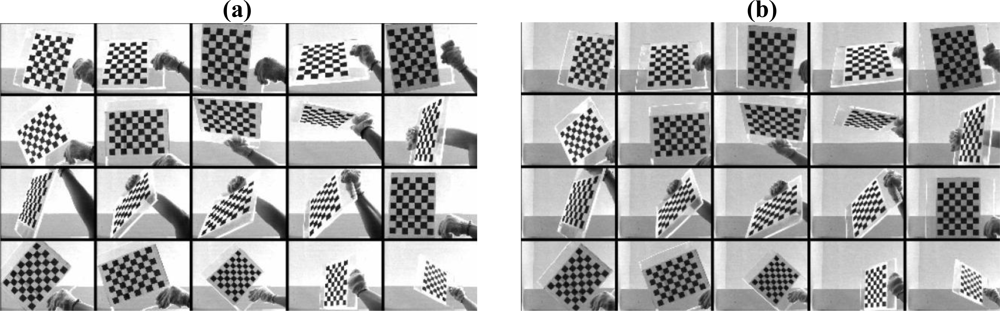
In order to obtain precise parameters of camera, the calibration pattern needs to take at least 5 and up to 20 pictures from different distances and angles simultaneously. As shown in Figure 5, the pictures of the chess board are taken by the left and the right camera respectively.
After the stereo images of the calibration patterns are achieved, the camera calibration tool is able to compute the intrinsic parameters and the extrinsic parameters of each camera.
3.3. Epipolar Geometry
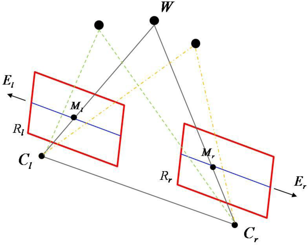
As shown in Figure 6, it is interesting to note that when the baseline ( ) is contained in both focal planes, that is, both image planes (Rl and Rr) are parallel to the baseline, the epipoles (Er and El) are at infinity and the epipolar lines, denoted by the blue lines on two image planes, are all horizontal.
In this special case, also called the standard setting, the epipolar lines corresponding to the same horizontal rows with the same y coordinate in both images and point correspondences are searched over these rows, and that simplifies the computation of stereo correspondences. The imaged points of three arbitrary 3D points are all on the same horizontal epipolar lines.
3.4. Epipolar Rectification
As mentioned, the standard setting has a great advantage of reducing the computation of stereo correspondences, but it cannot be obtained by real cameras. However, if the cameras’ calibration parameters are known, this problem could be overcome through the Epipolar Rectification. In this paper, the rectification algorithm presented by Fusiello et al. [15] is adopted.
The stereo rig can be calibrated by Bouguet’s stereo calibration tool, that is, the intrinsic and extrinsic parameters of both left and right cameras are known. Therefore, from Equation (1), the PPM of the left camera P̃ol and the PPM of the right camera P̃or can be written as:
Define a pair of new PPMs P̃nl and P̃nr as:
The row vectors of R are the X, Y, and Z axes, respectively, of the camera reference frame, expressed in the world coordinates.
According to Fusiello’s algorithm, the row vectors of R can be calculated as:
The new X axis is parallel to the baseline:
The new Y axis is orthogonal to X (mandatory) and to k̂:
The new Z axis is orthogonal to XY (mandatory):
In the calculation of the new Y axis, the vector k̂ is an arbitrary unit vector which makes the new Y axis orthogonal to the new X axis. In order to make the new Y axis orthogonal to both the new X axis and the old Z axis, k̂ is set to be the unit vector of the old Z axis.
To rectify the left and right images, the mapping relationships between the old PPMs and the new PPMs of the left and right images need to be known. Let us consider the left image as the example here.
For a 3D point w appears on the left and right cameras, the old left perspective projection m̃ol and the new left perspective projection m̃nl can be expressed as:
Because the optical center is not affected by rectification, Equation (18) can be expressed in its parametric form as:
Therefore:
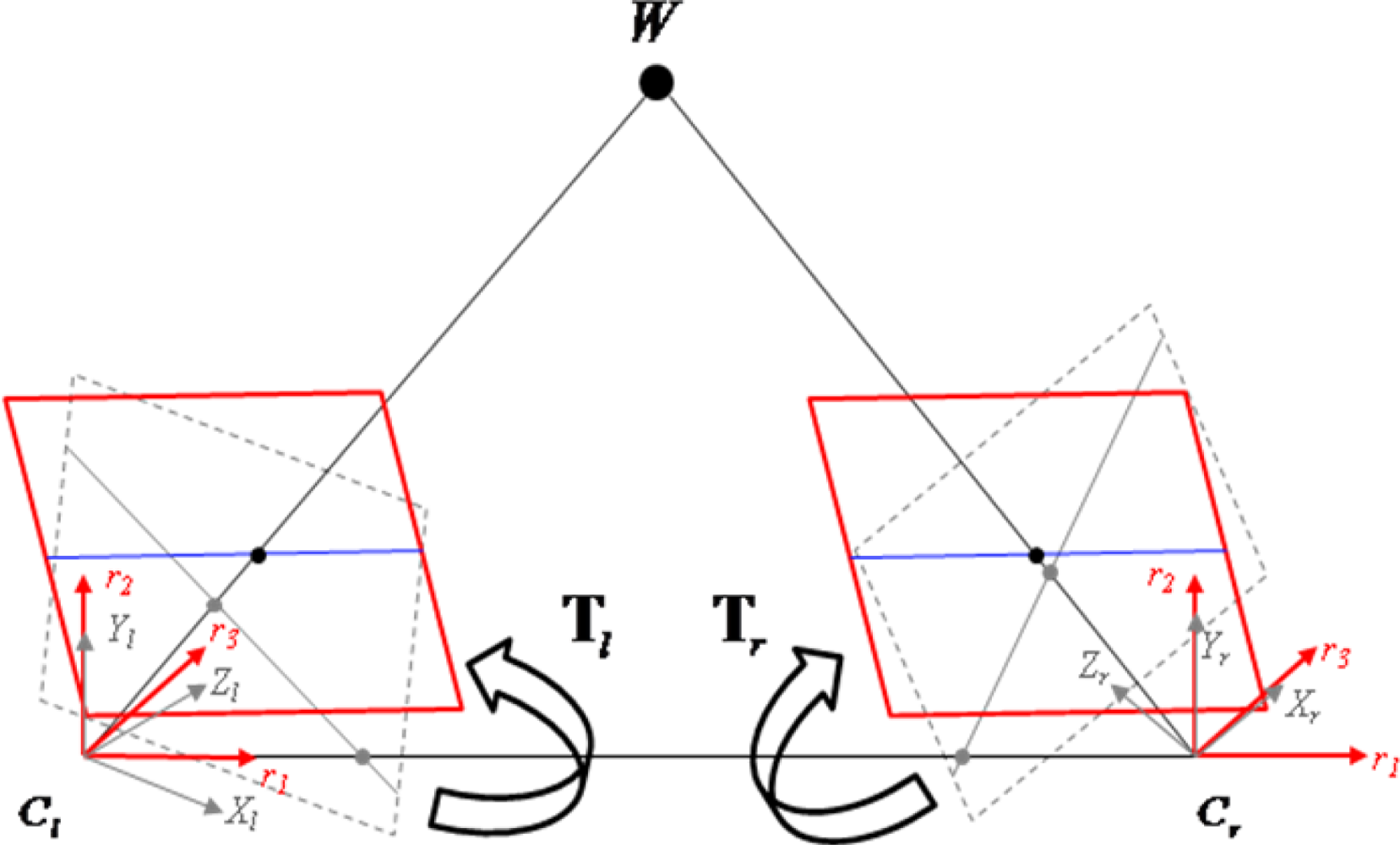
Now the rectification transformations Tl and Tr have been derived, which can be applied to the original left and right image, respectively, to get the rectified images. Figure 7 illustrates the above rectification transformation. Note that the bilinear interpolation is applied to interpolate the non-integer positions of the rectified images to the corresponding pixel coordinates of the original images.
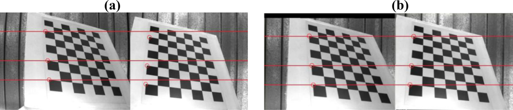
The image rectification includes the radial distortion correction [37] and the epipolar rectification [15] in this paper. Since both need to have the knowledge of camera parameters, Bouguet’s camera calibration toolbox of MATLAB [16] is used. The radial distortion correction and the epipolar rectification can be carried out, and the results are shown in Figure 8. Table 2 shows the intrinsic and extrinsic parameters of the stereo rig.
4. Target Detection
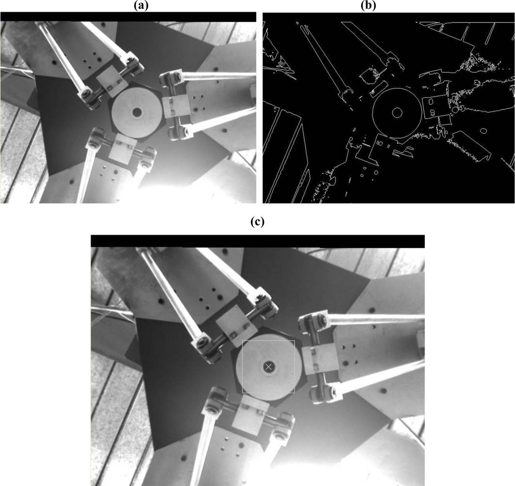
When detecting a circular object in a 3D space the circle radius is unknown. Although the circle radius can be known by pixel measurement in an image, it either needs to be re-measured when the circle radius changes, or the target has to be set in the vertical plane to maintain the same circle radius. It’s inconvenient and loses the generality. Hence, the ‘Pixel-to-Pixel’ circle detection algorithm developed by D. Scaramuzza et al. [23] is adopted in this paper. The experimental results of the target detection are shown in Figure 9. Note that the target detection algorithm is applied on the rectified left image. Figure 9(a) is the target required to be detected; Figure 9(b) is the image applied by the Laplacian edge detection to Figure 9(a); Figure 9(c) shows the result of target detection.
5. Stereo Tracking
The blocking matching is one of the best known methods for motion tracking and stereo matching due to its ease of implementation and less computational effort. The Sum of Square Difference (SSD) and the Sum of Absolute Difference (SAD) are the commonly used matching criteria for block matching. Because the SSD squares the intensity differences, it requires heavier computational burden than the SAD during the matching process. For the purpose of real-time stereo tracking, the SAD based stereo tracking is utilized:
Equation (23) expresses the SAD matching criterion, where fk is an image from the k frame; R is selected the reference block; (2n + 1) × (2n + 1) is the size of the reference block.
After the circle detection determined the location of the object at the previous frame, the reference block of size (2n + 1) × (2n + 1) centered on this location is created and stored in memory to search the best match (i.e., the SAD score has the minimum value) at the current frame in the searching window. Once the best match has been found, the current location of the object (xL,yL) in the left image can be tracked; in addition, the reference block is replaced by the best match to adapt the searching on the next frame. Figure 10 illustrates the block matching process mentioned above.
Assume that the left and right images have been rectified, so the reference block only searches horizontally along the epipolar line of the right image. The searching criterion is the same as the moving tracking; that is, the best match is determined at the location where the SAD score is the minimum.
When the best match has been found, the corresponding location of the object in the right image can be obtained. Figure 11 shows the stereo matching process. In Equation (24), the SAD score is used to estimate the similarity between the reference block Rl of the left image and right image Ir. The search for the best match is done consecutively along all possible candidates within the allowable disparity range dmin ≤ dc ≤ dmax :
Figure 12(a,c) shows the stereo tracking results at three arbitrary positions of the target, namely, positions A, B, and C. The reference block is defined as a 25 × 25 size rectangular block, and the size of searching window is 50 × 50 in the left image. For stereo matching on the right image, the row size of the horizontal scan-line is 20 ≤ xr ≤ 360. Once the first match is found, the row size of the horizontal scan-line becomes , where is the x-coordinates of the first match.
6. Measurement Correction
There are three major types of errors in the correlation-based stereo system, such as foreshortening error, misalignment error, and systematic error [38]. In order to correct the incorrect measuring results caused by these error sources, the stereo system needs to be calibrated. Figure 13 shows the measurement calibration method used in this thesis. A one-centimeter grid paper and a custom-made mechanism are used to calibrate the measurement results.
Table 3 is the error table of depth measurement, which shows the depth measurement error on each corresponding XW coordinate. Note that the blank in the table indicates that the target goes out the view field of the stereo rig.
By computing the standard deviations of depth errors on each XW coordinate, we know that the standard deviations are small; that is, the depth errors of the corresponding XW coordinates are closed to their mean. Therefore, the depth errors can be assumed to be the average depth error. Based on abovementioned ideas, the average depth measurement errors listed in Table 3 are plotted in Figure 14. Since the distribution of the average depth measurement errors is approximated linearly, the linear regression method is used to model the depth measurement error. The MATLAB curve fitting toolbox is used to compute the depth error model coefficients and the fitting residuals. Figure 14 shows the average depth measurement error and its approximated linear model. Equation (25) is the linear depth error model derived from MATLAB. Note that Ze indicates the average depth measurement error.
Table 4 shows that the original average depth errors of each corresponding XW are reduced to below 1.65 mm after the error correction using the linear error model and the greatest error is reduced to 3.45 mm.
7. Trajectory Measurement Experiment
Figure 15 shows the frame assignment of the stereo vision system where {XC, YC, ZC} is the camera frame and {X, Y, Z} is the end-effector frame. Since the measurement result of stereo vision system is with respect to the camera frame, it needs to be transformed to be with respect to the end-effector frame. The pose relationship between each frame is defined as a homogeneous transformation matrix as Equation (26) shown, where is the origin of the end-effector relative to the camera frame. Note that all the experiment results shown in the following sections are transformed using Equation (26) to be in the consistent coordinates with the end-effector frame:
7.1. Fifth Order Polynomial Trajectory
The desired end-effector trajectories in the Z-direction are given as a fifth order polynomial trajectory with stroke 100 mm in 3 seconds and a fifth order polynomial trajectory with stroke 200 mm in 5 s, respectively. Figure 16 shows the stereo vision measuring results of the fifth order polynomial trajectory with stroke 100 mm.
The stereo vision measuring results of X and Y coordinates at both strokes of fifth order trajectory are less than ±2 mm, and the stereo vision measuring results in the Z-coordinates show that the end-effector can be positioned to the desired stroke profile. Figure 17 shows the comparison of the desired trajectory and stereo vision measurement results. The end-effector can follow the given desired trajectory well.
7.2. Sinusoidal Trajectory
The desired trajectory of the end-effector in Z-direction in this section is planned to be a fifth order polynomial trajectory with stroke 150 mm at t ≤ 4 s, and a sinusoidal trajectory at 4 s ≤ t ≤ 20 s, with amplitude of 50 mm and frequency of 1 rad/s. Figure 18 shows the stereo vision measuring results of the sinusoidal trajectory, and Figure 19 shows the comparison of the desired trajectory and the stereo measurement results. The measurement results of X and Y coordinates of sinusoidal trajectory are less than ±4 mm, and the difference between the desired sinusoidal trajectory and the measuring results is approximately ±4 mm at the peak of sinusoidal trajectory, which results from the effect of systematic error of the stereo vision system or the vibration of the end-effector during trajectory tracking.
8. Conclusions
This paper proposes a stereo vision 3D position measurement system for a three-axial pneumatic parallel mechanism robot arm. The stereo vision 3D position measurement system serves to measure the 3D trajectories of the end-effector of the robot arm. To track the end-effector of the robot arm, the circle detection algorithm is used to detect the desired target and the SAD algorithm is used to track the moving target and to search the corresponding target location along the conjugate epipolar line in the stereo pair. After camera calibration, both intrinsic and extrinsic parameters of the stereo rig can be obtained, so images can be rectified according to camera parameters. Through the use of the epipolar rectification, the stereo matching process is reduced to a horizontal search along the conjugate epipolar line. Finally, 3D trajectories of the end-effector were computed by the stereo triangulation.
In the experiments of this paper, the stereo calibration results, the image rectification results, the circle detection results and the stereo tracking results were shown graphically. In the practical stereo vision measurement experiments, the measuring error of Z direction has been corrected first, and the corrected measurement results show that the maximum average error of Z direction can be reduced to 2.18 mm. After correcting the measurement error, the end-effector of the three-axial pneumatic parallel mechanism robot arm was planned to track the fifth order polynomial trajectory and the sinusoidal trajectory. These trajectories were then successfully measured and tracked by the stereo vision 3D position measurement system developed in this paper. Future work on the stereo vision 3D position measurement system proposed in this paper can be suggested. To broaden the field of view, a fisheye lens can be used. Using a position sensor such as a laser range finder to calibrate stereo vision system requires the sensor fusion data of laser and stereo vision, and should achieve more reliable and more accurate measurements.
Acknowledgments
This research was sponsored by the National Science Council of Taiwan under the grant NSC 99-2628-E-002-021.
References
- Rankin, A.L.; Huertas, A.; Matthies, L.H. Stereo vision based terrain mapping for off-road autonomous navigation. Proc. SPIE 2009, 7332, 733210–733210-17. [Google Scholar]
- Mischler, A. 3D Reconstruction from Depth and Stereo Image for Augmented Reality Application. M.Sc. Thesis,. Computer Graphics Group, Institute for Computer Engineering, Faculty IV, Technische Universität Berlin, Berlin, Germany, 2007. [Google Scholar]
- Richa, R.; Poignet, P.; Liu, C. Three-dimensional motion tracking for beating heart surgery using a thin-plate spline deformable model. Int. J. Robotic Res 2010, 29, 218–230. [Google Scholar]
- Wang, C.P. Automated Real-Time Object Detection and Recognition on Transportation Facilities; Exploratory Project, Civil Engineering,; University of Arkansas: Fayetteville, AR, USA, 2010. [Google Scholar]
- Lin, H.T. Design and Control of a Servo Pneumatic Three-axial Parallel Mechanism Arm. M.Sc. Thesis,. Department of Engineering Science and Ocean Engineering, National Taiwan University, Taipei, Taiwan, 2008. [Google Scholar]
- Peleg, A.; Weiser, U. MMX technology extension to the intel architecture. IEEE Micro 1996, 16, 42–50. [Google Scholar]
- Marr, D.; Poggio, T. Cooperative computation of Stereo Disparity. Science 1976, 194, 283–287. [Google Scholar]
- Pollard, S.B.; Mayhew, J.E.; Frisby, J.P. A stereo correspondence algorithm using a disparity gradient limit. Perception 1985, 14, 449–470. [Google Scholar]
- Scharstein, D.; Szeliski, R. A Taxonomy and Evaluation of Dense Two-Frame Stereo Correspondence Algorithms. Int. J. Comput. Vis 2002, 47, 4–72. [Google Scholar]
- Papadimitrious, D.V.; Dennis, T.J. Epipolar line estimation and rectification for stereo image pairs. IEEE Trans. Image Process 1996, 5, 672–676. [Google Scholar]
- Lee, K.L. Optimization of Fundamental Matrix and Euclidean Reconstruction. M.Sc. Thesis,. Institutes of Computer Science and Engineering, National Chiao Tung University, Hsinchu, Taiwan, 2002. [Google Scholar]
- Dornaika, F. Self-calibration of a stereo rig using monocular epipolar geometries. Patt. Recog 2007, 40, 2716–2729. [Google Scholar]
- Fusiello, A.; Irsara, L. Quasi-Euclidean Uncalibrated Epipolar Rectification. International Conference on Pattern Recognition, Tampa, FL, USA, December 8–11, 2008.
- Abraham, S.; Förstner, W. Fish-eye-stereo calibration and epipolar rectification. ISPRS J. Photogramm. Remote Sens 2005, 59, 278–288. [Google Scholar]
- Fusiello, A.; Trucco, E.; Verri, A. A compact algorithm for rectification of stereo pairs. Mach. Vision Appl 2000, 20, 16–22. [Google Scholar]
- Bouguet, J.Y.; Camera, Calibration. Toolbox for Matlab. Available online: http://www.vision.caltech.edu/bouguetj/calib_doc/index.html (22 November 2010).
- Zhang, Z. Flexible Camera Calibration by Viewing a Plane from Unknown Orientations. International Conference on Computer Vision, Corfu, Greece, September 20–27, 1999; pp. 666–673.
- Heikkilä, J.; Silvén, O. A Four-Step Camera Calibration Procedure with Implicit Image Correction. Proceedings of IEEE International Conference on Computer Vision and Pattern Recognition, San Juan, Puerto Rico, June 17–19, 1997; pp. 1106–1111.
- Duda, R.O.; Hart, P.E. Use of the hough transform to detect lines and curves in pictures. Commun. ACM 1972, 15, 11–15. [Google Scholar]
- Kimme, C.; Ballard, D.; Sklansky, J. Finding Circles by an Array of Accumulators. Commun. ACM 1975, 18, 120–122. [Google Scholar]
- Minor, L.; Sklansky, J. Detection and Segmentation of Blobs in Infrared Images. IEEE Trans. Sys. Man. Cyber 1981, SMC-11, 194–201. [Google Scholar]
- Rad, A.A.; Faez, K.; Qaragozlou, N. Fast Circle Detection Using Gradient Pair Vectors. Proceedings of Seventh Digital Image Computing: Techniques and Applications, Sydney, Australia, December 10–12, 2003.
- Scaramuzza, D.; Pagnottelli, S.; Valigi, P. Ball Detection and Predictive Ball Following Based on a Stereoscopic Vision System. Proceedings of the 2005 IEEE International Conference on Robotics and Automation, Barcelona, Spain, April 18–22, 2005; pp. 1573–1578.
- Inaba, M.; Hara, T.; Inoue, H. Stereo Viewer Based on Single Camera with View-Control Mechanisms. Proceedings of IEEE/RSJ International Conference on Intelligent Robots and Systems, Yokohama, Japan, July 26–30, 1993; pp. 1857–1865.
- Kaneko, T.; Hori, O. Feature Selection for Reliable Tracking using Template Matching. IEEE Computer Society Conference on CVPR, Madison, WI, USA, June 16–22, 2003.
- Tissainayagam, P.; Suter, D. Object tracking in image sequences using point features. Patt. Recog 2005, 38, 105–113. [Google Scholar]
- Bascle, B.; Deriche, R. Region Tracking Through Image Sequences. Proceedings of Fifth International Conference on Computer Vision, Cambridge, MA, USA, June 20–23, 1995; pp. 302–307.
- Comaniciu, D.; Ramesh, V.; Meer, P. Kernal-based object tracking. IEEE Trans. Patt. Anal. Mach. Int 2003, 25, 564–577. [Google Scholar]
- Matthews, I.; Ishikawa, T.; Baker, S. The template update problem. IEEE Trans. Patt. Anal. Mach. Int 2004, 26, 810–815. [Google Scholar]
- Canny, J.F. A computational approach to edge detection. IEEE Trans. Patt. Anal. Mach. Int 1986, 8, 679–698. [Google Scholar]
- Smith, S.M.; Brady, J.M. SUSAN—A new approach to low level image processing. Int. J. Comput. Vis 1997, 23, 45–78. [Google Scholar]
- Brown, M.Z.; Burschka, D.; Hager, G.D. Advances in computational stereo. IEEE Trans. Patt. Anal. Mach. Int 2003, 25, 993–1001. [Google Scholar]
- Kalomiros, J.; Lygouras, J. Comparative study of local SAD and dynamic programming for stereo processing using dedicated hardware. EURASIP J. Adv. Signal Process 2009, 2009. [Google Scholar] [CrossRef]
- Tao, T.; Koo, J.C.; Choi, H.R. A Fast Block Matching Algorithm for Stereo Correspondence. Proceedings of IEEE 2008 Conference on Cybernetics and Intelligent Systems, Chengdu, China, September 21–24, 2008; pp. 38–41.
- Faugeras, O.; Hotz, B.; Mattieu, H.; Vieville, T.; Zhang, Z.; Fua, P.; Theron, E.; Moll, L.; Berry, G.; Vuillemin, J.; et al. Real Time Correlation-Based Stereo: Algorithm, Implementations and Applications; INRIA Technical Report 2013; INRIA: Cedex, France, 1993. [Google Scholar]
- Su, Y.Y. A 12-bit Column-Parallel Cyclic Analog-to-Digital Converter for CMOS Image Sensor. M.Sc. Thesis,. Department of Electrical Engineering, National Cheng Kung University, Tainan, Taiwan, 2005. [Google Scholar]
- Devernay, F.; Faugeras, O. Straight lines have to be straight: automatic calibration and removal of distortion from scenes of structured environments. Mach. Vis. Appl 2001, 13, 14–24. [Google Scholar]
- Von Kaenel, P.; Brown, C.M.; Coombs, D.J. Detecting Regions of Zero Disparity in Binocular Images; Technical Report; Computer Science Department, University of Rochester: Rochester, NY, USA, 1991. [Google Scholar]
- Kuhl, A. Comparison of Stereo Matching Algorithms for Mobile Robots. M.Sc. Thesis,. Fakultät für Informatik und Automatisierung, Technische Universität Ilmenau, Ilmenau, Germany, 2004. [Google Scholar]


| Item | Specification | |
|---|---|---|
| CS8550Di CCD Camera | Image sensor | All Pixel’s Data Read-out Interline CCD |
| Video output pixels | 648(H) × 492(V) (Under non-interlace) | |
| Scanning area | 1/3 ” | |
| Scanning lines | 525 lines | |
| Interlace | 1/60 s Non-interlace mode 1/120 s 2:1 Interlace mode | |
| S/N | 52 dB(p-p)/rms | |
| Power source | DC12 V ± 10% | |
| Power consumption | Approx. 1.8 W | |
| Lens mount | C-MOUNT | |
| IMAQ PCI-1410 | Available Formats | RS-170/NTSC 30 frames/s interlaced CCIR/PAL 25 frames/s interlaced VGA 60 Hz, 640 × 480 resolution |
| Interface | PCI | |
| Channel | 4 | |
| Resolution | 8 or 10 bits | |
| Onboard Memory | 16 MB SDRAM | |
| Sampling Rate | 2 M∼40 MHz | |
| S/N | 56 dB | |
| Left Camera | Right Camera | ||||
|---|---|---|---|---|---|
| Focal Length | Horizontal | α = 848.80271 (pixel) | Focal Length | Horizontal | α = 850.84235 (pixel) |
| Vertical | β = 848.42222 (pixel) | Vertical | β = 851.00526 (pixel) | ||
| Skew | γ = 0 | Skew | γ = 0 | ||
| Principle Point | u0 = 323.29556 (pixel) v0 = 231.51767 (pixel) | Principle Point | u0 = 320.44027 (pixel) v0 = 254.04592 (pixel) | ||
| Distortion (Radial) | κ1 = −0.36358 κ2 = 0.14213 | Distortion (Radial) | κ1 = −0.23851 κ2 = 0.04721 | ||
| Extrinsic Parameters | Rotation | ||||
| Translation | (mm) | ||||
| XW | −80 | −60 | −40 | −20 | 0 | 20 | 40 | 60 | 80 | 100 | 120 |
|---|---|---|---|---|---|---|---|---|---|---|---|
| ZW | |||||||||||
| 415 | 1.93 | −1.02 | −3.88 | −6.68 | −9.41 | ||||||
| 435 | 2.23 | −0.07 | −4.52 | −5.59 | −9.87 | ||||||
| 455 | 6.06 | 2.02 | −0.64 | −3.21 | −5.73 | −9.44 | −13.08 | ||||
| 475 | 4.83 | 1.77 | −1.23 | −4.15 | −5.65 | −9.87 | −12.65 | ||||
| 495 | 9.69 | 6.05 | 2.52 | −0.88 | −4.17 | −5.77 | −9.11 | −12.24 | |||
| 515 | 10.31 | 4.38 | 2.32 | 0.47 | −3.31 | −9.06 | −10.68 | −12.16 | −15.87 | ||
| 535 | 9.24 | 4.14 | 1.59 | −2.39 | −4.29 | −8.13 | −9.98 | −12.46 | −16.24 | ||
| 555 | 12.01 | 7.12 | 4.25 | 1.73 | −0.91 | −7.42 | −8.25 | −9.98 | −13.94 | −18.14 | |
| 575 | 12.84 | 9.97 | 4.55 | 1.84 | −0.73 | −3.27 | −5.74 | −10.77 | −13.15 | −15.67 | |
| 595 | 19.14 | 12.93 | 9.8 | 6.69 | 3.84 | −1.8 | −4.54 | −7.34 | −10.08 | −12.68 | −15.37 |
| 615 | 18.63 | 15.22 | 8.37 | 5.18 | 2.1 | −1.1 | −4.12 | −7.15 | −10.14 | −13.01 | −15.91 |
| 635 | 16.18 | 12.45 | 8.85 | 4.58 | 1.81 | −1.61 | −5.04 | −4.97 | −8.81 | −11.43 | −14.53 |
| S.D. | 1.58 | 1.25 | 1.04 | 0.89 | 0.59 | 0.75 | 1.12 | 1.30 | 0.58 | 0.68 | 1.10 |
| Avg. Error | 17.98 | 13.09 | 9.17 | 5.07 | 2.14 | −0.99 | −4.33 | −6.67 | −9.85 | −12.68 | −15.96 |
| XW | −80 | −60 | −40 | −20 | 0 | 20 | 40 | 60 | 80 | 100 | 120 |
|---|---|---|---|---|---|---|---|---|---|---|---|
| ZW | |||||||||||
| 415 | 1.95 | −0.68 | 0.74 | 1.11 | |||||||
| 435 | 0.48 | 0.33 | 0.33 | 0.14 | 0.14 | ||||||
| 455 | 1.25 | −0.74 | 1.21 | 0.68 | 1.22 | 0.55 | |||||
| 475 | 0.39 | −0.3 | −0.51 | −0.13 | 0.02 | 0.31 | 0.62 | ||||
| 495 | 0.72 | 0.38 | 0.25 | 1.8 | 1.8 | 1.61 | 1.56 | 1.42 | |||
| 515 | 1.57 | 0.75 | 0.36 | −0.14 | 1.27 | 2.54 | 2.12 | 1.57 | |||
| 535 | 0.71 | 1.82 | 0.94 | −0.05 | 1.19 | 2.27 | 3.35 | 2.34 | 1.51 | ||
| 555 | 1.34 | −0.31 | 0.5 | 1.52 | 0.05 | 0.98 | 1.87 | 0.36 | 1.34 | −0.11 | |
| 575 | 2.26 | 0.48 | 1.16 | 1.68 | 2.43 | 0.53 | 1.17 | 1.77 | 2.46 | 0.62 | |
| 595 | −0.16 | 0.26 | 0.45 | 0.21 | −1.56 | 1.72 | 1.94 | −0.29 | 0.05 | 3.14 | 3.45 |
| 615 | −0.78 | −0.72 | −0.73 | 2.52 | −0.55 | −0.32 | −0.26 | 3.00 | 0.06 | 0.15 | 0.39 |
| 635 | 0.09 | −0.13 | −0.41 | 2.13 | −0.79 | −0.82 | −1.08 | 1.78 | 1.44 | 1.83 | 1.78 |
| Avg. Error | −0.28 | 0.60 | 0.31 | 1.11 | 0.27 | 0.42 | 0.67 | 1.37 | 1.06 | 1.65 | 1.27 |
© 2011 by the authors; licensee MDPI, Basel, Switzerland. This article is an open access article distributed under the terms and conditions of the Creative Commons Attribution license (http://creativecommons.org/licenses/by/3.0/).
Share and Cite
Chiang, M.-H.; Lin, H.-T.; Hou, C.-L. Development of a Stereo Vision Measurement System for a 3D Three-Axial Pneumatic Parallel Mechanism Robot Arm. Sensors 2011, 11, 2257-2281. https://doi.org/10.3390/s110202257
Chiang M-H, Lin H-T, Hou C-L. Development of a Stereo Vision Measurement System for a 3D Three-Axial Pneumatic Parallel Mechanism Robot Arm. Sensors. 2011; 11(2):2257-2281. https://doi.org/10.3390/s110202257
Chicago/Turabian StyleChiang, Mao-Hsiung, Hao-Ting Lin, and Chien-Lun Hou. 2011. "Development of a Stereo Vision Measurement System for a 3D Three-Axial Pneumatic Parallel Mechanism Robot Arm" Sensors 11, no. 2: 2257-2281. https://doi.org/10.3390/s110202257