State Derivation of a 12-Axis Gyroscope-Free Inertial Measurement Unit


Abstract
: The derivation of linear acceleration, angular acceleration, and angular velocity states from a 12-axis gyroscope-free inertial measurement unit that utilizes four 3-axis accelerometer measurements at four distinct locations is reported. Particularly, a new algorithm which derives the angular velocity from its quadratic form and derivative form based on the context-based interacting multiple model is demonstrated. The performance of the system was evaluated under arbitrary 3-dimensional motion.
1. Introduction
Inertial sensors have been widely used in various applications, including motion detection [1], body state estimation [2–4], navigation [5–7], microsurgery [8], rehabilitation [9], etc. Traditionally a standard inertial measurement unit (IMU) comprised of 3-axis linear acceleration measurement by accelerometers installed at center of mass (COM) and 3-axis angular velocity measurement by rate gyros readily provides complete six degree-of-freedom (DOF) motion-related measurements spanning the 3-dimensional space. For highly dynamic systems which favorably have angular acceleration measurements, to the best of our knowledge there is no off-the-shelf product available. One widely adopted approach to derive this state is by differentiation of rate gyro signals, together with the filter technique. The other approach is based on the principle of Newtonian Mechanics, which relates linear acceleration, angular acceleration, and angular velocity in a memoryless manner. Because of this characteristic, derivation of the angular acceleration by only the inertial sensors seems to be a feasible method [10].
The gyroscope-free inertial measurement unit (GF-IMU) [11–13] is one of the more popular IMU methods to achieve this goal. Compared to the traditional IMU, the GF-IMU utilizing only accelerometers includes several features such as low-cost, easy calibration, being less affected by temperature variations, and a simple mechatronic setup. In general, the GF-IMU is capable of deriving linear acceleration, angular acceleration, and angular velocity. Because the latter two states have integrative/derivative relation, a GF-IMU comprised of 6-axis measurements is theoretically capable of yielding all three states (i.e., 9 scalar unknowns). One of the typical configurations of sensors is to have a 3-axis acceleration measurement at the COM and three 1-axis measurements on the principal axes. However, the iterative computation between the derived angular acceleration and the integrated angular velocity can possibly deteriorate the fidelity of these two states. Padgaonkar et al. proposed a 9-axis acceleration measurement system capable of deriving bounded linear and angular acceleration [14]. Chen et al. proposed a novel 6-axis system which yielded a bounded angular acceleration [15]. The system was carefully evaluated [16] and improved by adding a 3-axis acceleration measurement [17]. In general, due to the quadratic formulation of angular velocity in the rigid body dynamics, the derivation of this state in the 9-axis IMU faces the sign ambiguity problem [18]. This dilemma can be solved by comparing it to the estimated angular velocity which is integrated from the angular acceleration measurement [19] or by adding the redundant measurements to the IMU, for example, to increase the measurements to 12-axis [20]. Parsa et al. later developed an original all-accelerometer IMU which requires twelve 1-axis accelerometers mounted at specific locations on the surfaces of a cube. The system is capable of deriving all three states in which the angular velocity was derived through an optimization procedure from six measured inputs in the quadratic form [21]. Schopp et al. reported another novel 12-axis IMU which was constructed by twelve 1-axis accelerometers in different configurations and utilized an Unscented Kalman Filter (UKF) to yield all three states simultaneously [22].
Previously we had installed a 12-axis IMU composed of four 3-axis accelerometers at four distinct locations on the robot RHex [23], together with some custom-made leg sensors [24], to perform sensor data fusion for full body state estimation in this hexapod robot with dynamical gait [25]. Based on the rigid-body dynamics and matrix theory, the developed 12-axis IMU is theoretically capable of deriving all three states. However, limited available space on the RHex for sensor installation at that time constrained the configuration of the IMU far from the optimum level. Only the linear and angular accelerations were available for further analysis and no angular velocity developments were performed.
Here, we report on the state derivation and performance evaluation of the 12-axis IMU with optimal configuration in the sense of matrix operation, allowing the system to yield all three states. Particularly, a new algorithm which derives the angular velocity is reported. Basically, the state is estimated by the mixed signals from its quadratic form and derivative form based on the context-based interacting multiple models (IMM) [26]. The algorithm requires low computation power suitable for real-time derivation of the state. The proposed 12-axis IMU in its new configuration was tested under 3-dimensional random motion with various magnitudes, and its performance was evaluated by comparing to the results from the traditional IMU installed at the COM.
Section 2 briefly reviews the construction of the 12-axis IMU based on the analysis of rigid body dynamics. Section 3 describes the derivation of the angular velocity by the context-based IMM in detail. Section 4 reports the results of experimental evaluation, and Section 5 concludes the work.
2. Construction of the 12-Axis IMU
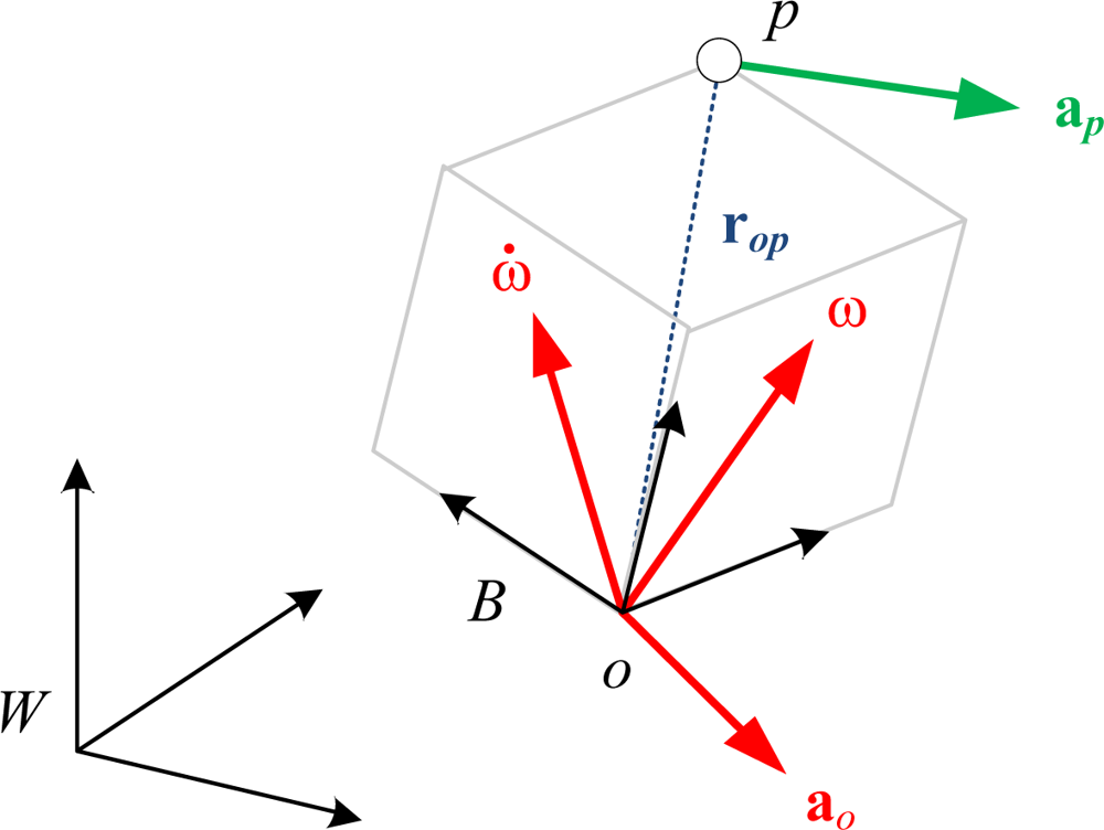
A brief review regarding construction of the 12-axis IMU is described in this section [25]. As shown in Figure 1, the acceleration vector, ap, of a point, p, rigidly attached to an accelerating body frame B with origin o, in the inertial frame, W, is a function of the body’s angular velocity, ω, angular acceleration, ω̇, and translational acceleration of the body origin, ao, represented by:
With the quadratic representation of the angular velocity:
Equation (1) appears to be linear with these 12 scalar unknowns:
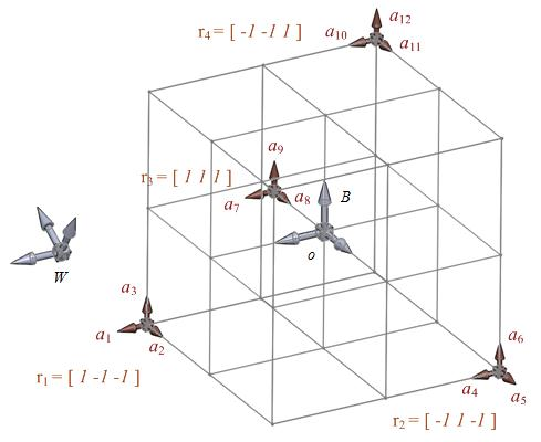
Presumably four 3-axis accelerometers are installed at point pj, j=1,2,3,4 with known ropj, j=1,2,3,4 :
The unknown body states can now be derived by the matrix operation:
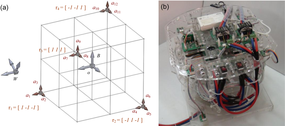
Equation (7) reveals that the extraction of the desired state, xvar, now depends on the rank and numerical condition of the “structure matrix”, S(rm), which is solely a function of the positions of accelerometers, rm. Previously the numerical exploration pointed out that allocation of the four sensors shown in Figure 2(a) yields the best condition number of S(rm), square root of 2. It indicates that this configuration is the most appropriate for matrix inversion [25], and the computation error induced by the matrix inversion is small. Therefore the new experimental setup shown in Figure 2(b) was built according to this configuration for the following analysis. Please note that the construction and inversion of the structure matrix S(rm) only needs to be done once and can be computed offline after the positions and orientations of the accelerometers are determined.
3. Derivation of the Angular Velocity from the 12-Axis GF-IMU
Section 2 shows that in the real-time process the unknown body state xvar in the proposed 12-axis GF-IMU can be derived from the 12 sensed scalar accelerations multiplied with the inversed structure matrix shown in Equation (7). In xvar, the linear and angular accelerations are readily derived though the angular velocity in its exact form is still unsolved and requires further computation. In the current formulation, two sensed sources are available for this computation. One is from the angular acceleration, the 4th–6th terms of xvar shown in Equation (4), which is the derivative of the desired state. The other is from the last six terms of xvar, which is the quadratic form of the desired one. Because in the empirical setup the developed algorithm is executed by the commercial computers, the representation is in the discrete domain in the following sections.
3.1. The Primitive Derivation of the Angular Velocity
To derive the angular velocity from the available angular acceleration, ωint, the trapezoid integration is the preferred method:
The angular velocity derived from its quadratic form (hereafter referred to as the “quadratic method”) has non-drift nature; however, the trade-off is the sign ambiguity problem, meaning to select the correct answer from multiple potential choices resulted from “square-root” computations. More specifically, assuming the first three quadratic terms shown in Equation (3) are chosen:
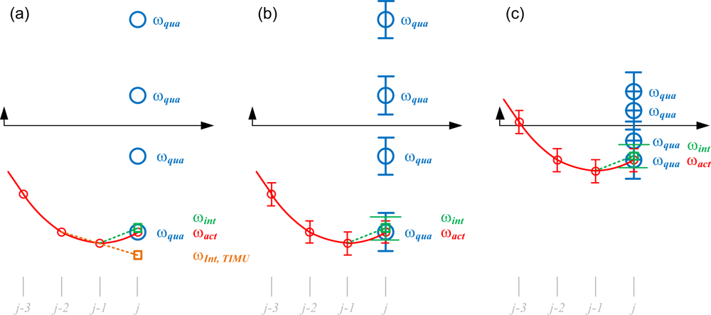
Practically, the quadratic method described above is likely to select an incorrect answer while the magnitude of the actual angular velocity, ωact, is small. If the derived ωj−1 at time stamp j − 1 is precise, the most likely cause of estimation error of ωj at time stamp j “in the perfect world” is the process of trapezoid integration, which assumes the acceleration is constant during that time interval. As depicted in Figure 3(a), the actual motion pattern may vary in a very fast manner, and the angular acceleration derived from the 12-axis GF-IMU catches the instant value at the sampled time stamp because of the memoryless computation shown in Equation (7). The discrepancy between the instant and average accelerations during time stamp j results in the estimation error of the initial-guess, ωint,j. This phenomenon in the traditional IMU (TIMU) which derives the angular acceleration by the differentiation of the angular velocity signal is even worse since the differentiation process introduces the noise and delay as shown in Figure 3(a). In the empirical world the situation is even more severe due to signal noises and accumulated digitization round-off errors during computation. For example, the estimated ωj−1 at the j − 1 time stamp may already have certain estimation error, and the calculated angular acceleration and quadratic angular velocity shown in Equation (7) also have certain errors due to digitized matrix inversion and noisy sensor signals as depicted in Figure 3(b). Both empirical effects strongly affect the accuracy of 1-out-of-8 selection process, especially when the magnitude of the actual angular velocity ωact is small, as depicted in Figure 3(c) where multiple choices of ωqua may fall into the estimated ranges. In addition, because the estimation process is iterative, one incorrect estimate may badly affect the correctness of future estimates. Therefore it can be concluded that the quadratic method is suitable while the magnitude of quadratic sums, a, b, and c, are either very close to zero or large (i.e., not small).
In summary, neither one of the two methods is individually capable of yielding a correct estimation of the angular velocity. Because of the complementary characteristics between them, it is intuitive to fuse signals from these two methods to yield a better angular velocity estimate, ω12-axis.
3.2. Context-Based Interacting Multiple Models
A better estimation of the angular velocity can be achieved by the adequate combination of the signals derived from the integration and quadratic methods. The process can be categorized within the domain of Interacting Multiple Models (IMM) [27,28], which generally calculates the accuracy of all models in a stochastic manner and mixes the estimated signals from all sources in a weighted manner to produce the correct estimate. Because executing the covariance of all models requires certain computation power as well as the performance of the models for specific scenarios may not be fairly judged by simple Gaussian assumptions, the context-based IMM [26] is adopted in the developed algorithm, which introduces the pre-selected contexts as the basic judgment for signal mixture from multiple models.
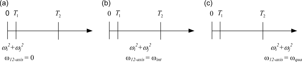
The development shown in the previous sub-section indicates that the quadratic method is effective while the magnitude of the angular velocity is either close to zero or very large. Therefore, two thresholds, T1 and T2, are selected as the contexts. T1 is the boundary where the estimated angular velocity should be treated as zero, and T2 is the boundary where the quadratic method is effective. These two contexts divide the range of quadratic sums, a, b, and c, into three sections as depicted in Figure 4. While 0 ≤ ωi2 + ωj2 ≤ T1 as shown in Figure 4(a), referred to as the zero model, one can set the angular velocity to zero. While ωi2 + ωj2 ≥ T2 as shown in Figure 4(c), referred to as the quadratic model, one can obtain the angular velocity by the quadratic method. While T1 ≤ ωi2 + ωj2 ≤ T2 as shown in Figure 4(b), referred to as the integration model, one adopts the integration method.
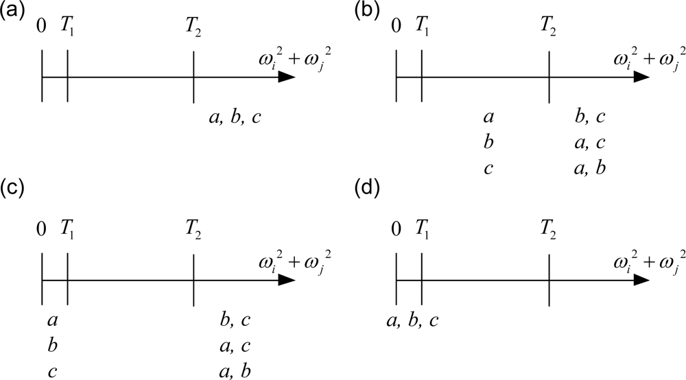
Each of the quadratic sums, a, b, or c, can reside in three possible sections shown in Figure 4, so there are twenty-seven possible combinations. Because the equations shown in Equation (9) are coupled, further categorization and treatment is detailed as follows.
Case 1. a, b, c ≥ T2
When a, b, c ≥ T2 as shown in Figure 5(a), ωact is far away from zero along all three principal directions. In this case the estimated ω12-axis is determined by the quadratic method:
Case 2. T1 ≤ a < T2 and b, c ≥ T2
When T1 ≤ a < T2 and b, c ≥ T2 as shown in Figure 5(b), it is reasonable to conclude that ωact,z is far away from zero and ωact,x and ωact,y are likely to have moderate magnitudes. Therefore both methods are utilized in this case:
Similarly, both T1 ≤ b < T2, a, c ≥ T2 and T1 ≤ c < T2, a, b ≥ T2 are within this case.
Case 3. 0 ≤ a < T1 and b, c ≥ T2
When 0 ≤ a < T1 and b, c ≥ T2 as shown in Figure 5(c), it can be concluded that ωact,z has a large magnitude but ωact,x and ωact,y are close to zero. Therefore only the former requires computation by the quadratic method:
Similarly, both 0 ≤ b < T1, a, c ≥ T2 and 0 ≤ c < T1, a, b ≥ T2 are within this case.
Case 4. 0 ≤ a, b, c < T1
When 0 ≤ a, b, c < T1 as shown in Figure 5(d), it is reasonable to set all components to zero:
Besides the four cases shown above, there are nineteen combinations left undetermined. Because there is no clear trend to judge the adequateness of the quadratic method in these combinations, the estimated angular velocity ω12-axis is derived from the integration method (i.e., ω12-axis = ωint). If the computed a, b, or c appears in an unreasonable less-than-zero value due to empirical computation error, the estimated angular velocity ω12-axis is also derived from the integration method (i.e., ω12-axis = ωint, the quadratic sums are not utilized in the computation in this time stamp).
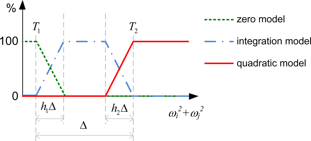
The proposed estimation shown in the previous paragraph has the “hard switching” nature. This implies an unreasonable situation because the trustworthiness of the models has a sharp boundary. Technically, suddenly switching the estimation from one method to another also introduces a signal discontinuity problem. Therefore the “soft switching” technique is adopted, which defines the probability of each model in a continuous manner as shown in Figure 6. When ωi2 + ωj2 is close to T1, ω12-axis is designed to be the linear combination of zero and ωint :
3.3. Brief Discussion
The algorithm reported in the previous sub-section utilizes the first three terms shown in Equation (3) to recover the angular velocity. The last three terms can also be utilized to perform the quadratic inversion. Assuming the quadratic multiplication is labeled as:
Because of the multiplication characteristics there are only two candidates instead of eight. This reveals that if one sign of ωi, i=x,y,z is selected, the other two will be determined. However, empirically the sign determination is tricky and no obvious model can be constructed. Thus this approach is not adopted in the development. Another method is to construct the complete squares by utilizing all six terms shown in Equation (3):
Though the sensed signals shown in Equation (7) are utilized in a more thorough manner, the strategy of setting adequate contexts is also not clear in this case. For example, the advantage of the zero model does not exist in this case because the setting of ωx + ωy = 0 can only reveal that ωx and ωy are in opposite sign with no magnitude information. Thus this approach is not adopted in the development either.
4. Experimental Evaluation
The experimental apparatus shown in Figure 2(b) was utilized for experimental evaluation of the proposed 12-axis system. The required sensory measurements were obtained from four 3-axis accelerometers (ADXL330, ±3g, Analog Device) installed at the specific configuration shown in Figure 2(a). In addition, a traditional IMU composed by one 3-axis accelerometer (ADXL330) and three 1-axis rate gyros (ADXRS610, ±3000/s, Analog Device) was also mounted at the COM for performance comparison. A real-time embedded control system (sbRIO-9632, National Instruments) running at 500 Hz was in charge of sensor signal collection. All of the analog input channels of the sbRIO have ±10 V range and 16-bit A-to-D resolutions. Random motions with varied magnitudes were applied to the experimental apparatus during experiments and the following analysis was based on the measured data.
4.1. Selection of Contexts T1 and T2
The context T1 represents the boundary which sets the estimated angular velocity ω12-Axis at zero. It is not reasonable to set a large T1 as it would force ω12-Axis to be zero when it is not. On the other hand, a very small T1 yields very little data that qualifies for this criterion. Empirically it is determined by the noise level of the sensors as well as the precision of the digitized computation. T1 is set around 0.1 in the experiments.
The context T2 determines the magnitude level where the angular velocity can be effectively determined by quadratic methods instead of the integration method. Therefore small T2 easily yields the wrong selection from the eight candidates. Large T2 forces the data to be computed by integration, and the data drift appears when the time duration of the angular velocity computed in this method is long. Therefore a study on how to correctly choose the right T2 is performed and detailed as follows.
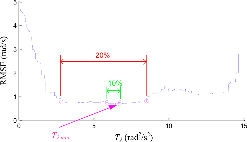
Figure 7 plots the typical Root-mean-squared Error (RMSE) vs. T2 based on one of the experimental data, where the RMSE is the comparison between the estimated angular velocity, ω12-Axis, and that measured by the traditional IMU, ωTIMU. The RMSE shown in the plot is the summed result of its three scalar components. The plot indicates that the RMSE is relatively large when T2 is small, when the quadratic method is over trusted. It also indicates that RMSE is relatively large when T2 is large. In this setting most of the estimates were done by the integration method and the data drift was observed. The wide and flat bottom of the curve shown in Figure 7 is also observed in other data sets, which indicates that there exists a wide selectable range of T2 values which yields similar performance, as the best RMSE happened at T2 min. For example, if the acceptable RMSE is bounded by an extra 20% of the best RMSE, the selectable range of T2 is spanned from 3 to 9.
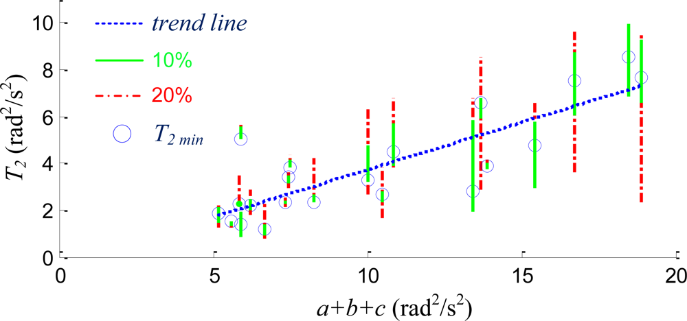
Figure 8 plots the variation of T2 min (blue circle) vs. the average level of the motion, which is quantitatively defined as the summation of the quadratic sums, a + b + c. Instead of defining the level of motion directly in the angular velocity, quadratic sums are utilized since these sums are available right after the multiplication of the inversed matrix to the sensory inputs shown in Equation (7). Because the errors resulted from the matrix inversion and noises due to empirical sensor readings are usually scaled with the magnitude of the signals, the selected T2 should increase as the magnitude of motion increases. The blue linear trend line with positive slope also confirms this phenomenon. The plot also reveals that the tolerable 10% or 20% increase of RMSE intersects with the linear trend line. Because the lengths of 20% lines are large and the slope of the trend line is small, the computation error of a + b + c has very little effect on the quantitative measure of the trend line. Thus the adequate T2 can be easily obtained according to the equation of the trend line when the quadratic sums, a, b, and c, are given. This plot suggests that the selection of T2 can be achieved by the given quadratic sums and the trend line, and the RMSE comparison test which requires the gyroscope input shown in Figure 7 is not necessary. The selected T2 is fixed for the followed real-time estimation.
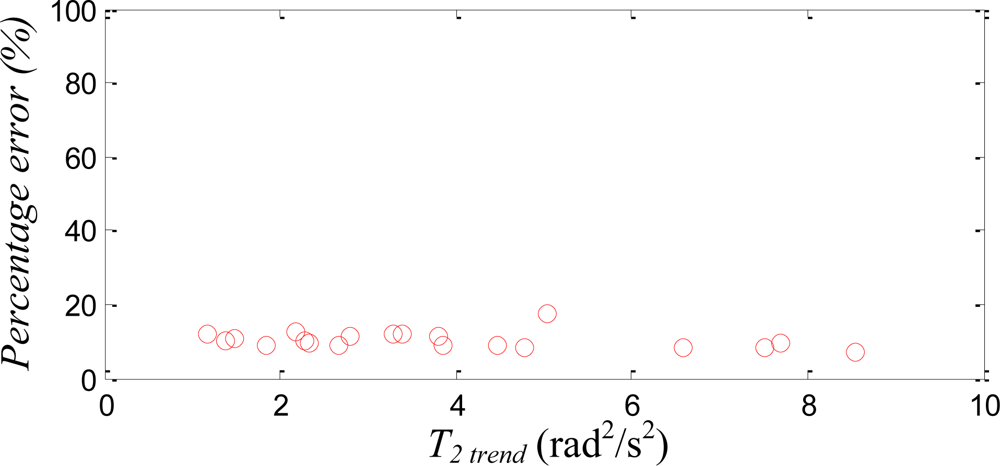
In order to quantitatively evaluate the usability of the trend line, instead of using T2 min as the context, Figure 9 plots the percentage error of the estimated angular velocity versus T2 trend, which is the selected T2 calculated from the trend line with given quadratic sums. Percentage error is calculated as the ratio of the RMSE to the maximum magnitude at that experiment trial, where the RMSE is the comparison between the estimated angular velocity, ω12-Axis, and that measured by the traditional IMU, ωTIMU. Figure 9 indicates that the computed T2 from trend line performs adequately; the percentage errors are mostly around 12% or less.
4.2. Performance of the State Derivation from the 12-Axis GF-IMU
In the experimental evaluation the apparatus was moved arbitrarily in the 3-dimensional space; thus the linear and angular accelerations along all three principal axes could be induced in the test. Before the sensor readings were imported into Equation (5), the raw accelerometer readings were filtered by Chebyshev filters and gravity-compensated by the readings of the 2-axis inclinometer. Table 1 lists the statistical summary of the experiments where the RMSEs were the comparisons between the estimated state of ω12-Axis and the measured state from the traditional IMU installed at the COM, ωTIMU. The angular acceleration of the traditional IMU is obtained by differentiation of the angular velocity, followed by filtered with a Chebyshev filter. Figure 10 plots one typical result of the experiment. Figure 10(a) confirms that though the sensors of the proposed 12-axis GF-IMU (thin red solid lines) are not located at the COM, they can indeed recover the COM linear acceleration. Figure 10(b) shows that the angular acceleration can also be correctly derived by the 12-axis GF-IMU. Figure 10(c) reveals that though several unmatched sections exist between the 12-axis GF-IMU and the traditional IMU readings, the proposed algorithm in general can indeed recover the angular velocity along with all three principal directions. The discrepancy either resulted from (i) the accumulated integration error where the magnitude of the quadratic sums fell into the integration model for too long or (ii) the incorrect selection of the angular velocity in the quadratic model.
Figure 11 compares the performance of three different methods: integration method, quadratic method, and the proposed method. Figure 10(c) reveals that the angular velocity derived from the proposed method matches closely to the readings from the traditional IMU, so in Figure 11 the performance of the latter one is skipped for clear presentation. Figure 11 shows that the angular velocity derived from the integration method drifts over time as expected. In contrast, the angular velocity derived from the quadratic method is bounded. However, the 1-out-of-8 selection process of the quadratic method is likely to select an incorrect answer while the magnitude of the signal is small. In addition, because the estimation process is iterative, one incorrect estimate may badly affect the correctness of future estimates until at certain moment the correct selection moves the estimates back to the right track. Figure 11 indicates that the proposed method with right mixture between the integration and the quadratic methods yields the adequate estimation.
Figure 12 shows the timings where the switching between two methods takes place. The 15-sec data had 7,500 sampled data points, and the proposed method switched around 100 times.
5. Conclusions
We have investigated a 12-axis inertial measurement unit that utilizes four 3-axis linear acceleration measurements from accelerometers installed at four distinct locations. We have developed a new algorithm which derives the angular velocity by mixing the signals from its quadratic form and its derivative form via the context-based interacting multiple models. The performance of the system was evaluated while the system was under arbitrary 3-dimensional motion. By adequately-choosing two contexts, the angular velocity can indeed be recovered. In the meantime, the linear and angular accelerations are correctly estimated as well, which confirmed that the COM acceleration state can be derived even though the sensors are not installed at that specific spot.
We are in the process of investigating a sensor fusion scheme of the reported system with other position and orientation sensors with the intention of constructing an observable system capable of accurate full body state estimation for analysis of dynamic locomotion in legged robots.
Acknowledgments
This work is supported by the National Science Council (NSC), Taiwan, under contract NSC 98-2218-W-002-034. The authors wish to express their gratitude to the National Instruments’ Taiwan Branch for their kind support of this study with equipment and technical consultation.
References
- Yang, CC; Hsu, YL. A Review of Accelerometry-Based Wearable Motion Detectors for Physical Activity Monitoring. Sensors 2010, 10, 7772–7788. [Google Scholar]
- Hernandez, W. Robust Multivariable Estimation of the Relevant Information Coming from a Wheel Speed Sensor and an Accelerometer Embedded in a Car under Performance Tests. Sensors 2005, 5, 488–508. [Google Scholar]
- Giansanti, D; Macellari, V; Maccioni, G; Cappozzo, A. Is It Feasible to Reconstruct Body Segment 3-D Position and Orientation Using Accelerometric Data? IEEE Trans. Biomed. Eng 2003, 50, 476–483. [Google Scholar]
- Tan, UX; Veluvolu, KC; Latt, WT; Shee, CY; Riviere, CN; Ang, WT. Estimating Displacement of Periodic Motion with Inertial Sensors. IEEE Sens. J 2008, 8, 1385–1388. [Google Scholar]
- Park, SK; Suh, YS. A Zero Velocity Detection Algorithm Using Inertial Sensors for Pedestrian Navigation Systems. Sensors 2010, 10, 9163–9178. [Google Scholar]
- Lai, YC; Jan, SS; Hsiao, FB. Development of a Low-Cost Attitude and Heading Reference System Using a Three-Axis Rotating Platform. Sensors 2010, 10, 2472–2491. [Google Scholar]
- Barshan, B; Durrantwhyte, HF. Inertial Navigation Systems for Mobile Robots. IEEE Trans. Robotics Automat 1995, 11, 328–342. [Google Scholar]
- Ang, WT; Khosla, PK; Riviere, CN. Nonlinear Regression Model of a Low-g MEMS Accelerometer. IEEE Sens. J 2007, 7, 81–88. [Google Scholar]
- Banala, SK; Agrawal, SK; Kim, SH; Scholz, JP. Novel Gait Adaptation and Neuromotor Training Results Using an Active Leg Exoskeleton. IEEE-ASME Trans. Mechatron 2010, 15, 216–225. [Google Scholar]
- Lin, PC; Lu, JC; Tsai, CH; Ho, CW. Design and Implementation of a 9-Axis Inertial Measurement Unit. IEEE Trans Mechatron 2011. in press.. [Google Scholar]
- Angeles, G. Fundamentals of Robotic Mechanical Systems: Theory, Methods, and Algorithms, 3rd ed; Springer: Berlin, Germany, 2006. [Google Scholar]
- Cardou, P; Angeles, J. Estimating the Angular Velocity of a Rigid Body Moving in the Plane from Tangential and Centripetal Acceleration Measurements. Multibody Syst. Dyn 2008, 19, 383–406. [Google Scholar]
- Cardou, P; Angeles, J. Linear Estimation of the Rigid-Body Acceleration Field from Point-Acceleration Measurements. J Dyn Syst Meas Control-Trans ASME 2009. [Google Scholar] [CrossRef]
- Padgaonkar, AJ; Krieger, KW; King, AI. Measurement of Angular Accelerarion of a Rigid Body Using Linear Accelerometers. Trans. ASME J. Basic Eng 1975, 42, 552–556. [Google Scholar]
- Chen, JH; Lee, SC; Debra, DB. Gyroscope Free Strapdown Inertial Measurement Unit by 6 Linear Accelerometers. J. Guid. Control Dyn 1994, 17, 286–290. [Google Scholar]
- Tan, CW; Park, S. Design of Accelerometer-Based Inertial Navigation Systems. IEEE Trans. Instrum. Meas 2005, 54, 2520–2530. [Google Scholar]
- Park, S; Tan, CW; Park, J. A Scheme for Improving the Performance of a Gyroscope-Free Inertial Measurement Unit. Sens. Actuat. A-Phys 2005, 121, 410–420. [Google Scholar]
- Genin, J; Hong, JH; Xu, W. Accelerometer Placement for Angular Velocity Determination. J. Dyn. Syst. Meas. Control-Trans. ASME 1997, 119, 474–477. [Google Scholar]
- Parsa, K; Angeles, J; Misra, AK. Rigid-Body Pose and Twist Estimation Using an Accelerometer Array. Arch. Appl. Mech 2004, 74, 223–236. [Google Scholar]
- Zappa, B; Legnani, G; van den Bogert, AJ; Adamini, R. On the Number and Placement of Accelerometers for Angular Velocity and Acceleration Determination. J. Dyn. Syst. Meas. Control-Trans. ASME 2001, 123, 552–554. [Google Scholar]
- Parsa, K; Lasky, TA; Ravani, B. Design and Implementation of a Mechatronic, All-Accelerometer Inertial Measurement Unit. IEEE-ASME Trans. Mechatron 2007, 12, 640–650. [Google Scholar]
- Schopp, P; Klingbeil, L; Peters, C; Manoli, Y. Design, Geometry Evaluation, and Calibration of a Gyroscope-Free Inertial Measurement Unit. Sens. Actuat. A-Phys 2010, 162, 379–387. [Google Scholar]
- Saranli, U; Buehler, M; Koditschek, DE. RHex: A Simple and Highly Mobile Hexapod Robot. Int. J. Robotics Res 2001, 20, 616–631. [Google Scholar]
- Lin, PC; Komsuoglu, H; Koditschek, DE. A Leg Configuration Measurement System for Full-Body Pose Estimates in a Hexapod Robot. IEEE Trans. Robotics 2005, 21, 778–778. [Google Scholar]
- Lin, PC; Komsuoglu, H; Koditschek, DE. Sensor Data Fusion for Body State Estimation in a Hexapod Robot with Dynamical Gaits. IEEE Trans. Robotics 2006, 22, 932–943. [Google Scholar]
- Skaff, S; Rizzi, AA; Choset, H; Lin, P-C. A Context-Based State Estimation Technique for Hybrid Systems. Proceedings of IEEE International Conference on Robotics and Automation (ICRA), Barcelona, Spain, 18–22 April 2005; pp. 3935–3940.
- Mazor, E; Averbuch, A; Bar-Shalom, Y; Dayan, J. Interacting Multiple Model Methods in Target Tracking: A Survey. IEEE Trans. Aerosp. Electron. Syst 1998, 34, 103–123. [Google Scholar]
- Chang, CB; Tabaczynski, JA. Application of State Estimation to Target Tracking. IEEE Trans. Autom. Control 1984, 29, 98–109. [Google Scholar]


| Linear acceleration (m/s2) | Angular acceleration (rad/s2) | Angular velocity (rad/s) | ||||||
|---|---|---|---|---|---|---|---|---|
| ax | ay | az | ω̇x | ω̇y | ω̇z | ωx | ωy | ωz |
| 0.1359 | 0.0933 | 0.1296 | 0.4985 | 0.7691 | 1.4188 | 0.3953 | 0.2301 | 0.2593 |
© 2011 by the authors; licensee MDPI, Basel, Switzerland. This article is an open access article distributed under the terms and conditions of the Creative Commons Attribution license (http://creativecommons.org/licenses/by/3.0/).
Share and Cite
Lu, J.-C.; Lin, P.-C. State Derivation of a 12-Axis Gyroscope-Free Inertial Measurement Unit. Sensors 2011, 11, 3145-3162. https://doi.org/10.3390/s110303145
Lu J-C, Lin P-C. State Derivation of a 12-Axis Gyroscope-Free Inertial Measurement Unit. Sensors. 2011; 11(3):3145-3162. https://doi.org/10.3390/s110303145
Chicago/Turabian StyleLu, Jau-Ching, and Pei-Chun Lin. 2011. "State Derivation of a 12-Axis Gyroscope-Free Inertial Measurement Unit" Sensors 11, no. 3: 3145-3162. https://doi.org/10.3390/s110303145