A Vocal-Based Analytical Method for Goose Behaviour Recognition

Abstract
: Since human-wildlife conflicts are increasing, the development of cost-effective methods for reducing damage or conflict levels is important in wildlife management. A wide range of devices to detect and deter animals causing conflict are used for this purpose, although their effectiveness is often highly variable, due to habituation to disruptive or disturbing stimuli. Automated recognition of behaviours could form a critical component of a system capable of altering the disruptive stimuli to avoid this. In this paper we present a novel method to automatically recognise goose behaviour based on vocalisations from flocks of free-living barnacle geese (Branta leucopsis). The geese were observed and recorded in a natural environment, using a shielded shotgun microphone. The classification used Support Vector Machines (SVMs), which had been trained with labeled data. Greenwood Function Cepstral Coefficients (GFCC) were used as features for the pattern recognition algorithm, as they can be adjusted to the hearing capabilities of different species. Three behaviours are classified based in this approach, and the method achieves a good recognition of foraging behaviour (86–97% sensitivity, 89–98% precision) and a reasonable recognition of flushing (79–86%, 66–80%) and landing behaviour(73–91%, 79–92%). The Support Vector Machine has proven to be a robust classifier for this kind of classification, as generality and non-linear capabilities are important. We conclude that vocalisations can be used to automatically detect behaviour of conflict wildlife species, and as such, may be used as an integrated part of a wildlife management system.1. Introduction
In many parts of the world, damage caused by wildlife creates significant economic challenges to human communities. Since human-wildlife conflicts are increasing [1] the development of cost-effective methods for reducing damage or conflict levels is important in wildlife management. A wide range of devices to detect and deter animals causing conflict are used in wildlife damage management, although their effectiveness is often highly variable [2]. Present scaring devices are often activated electronically, through detection of motion and/or body heat (e.g., infrared sensors, Gilsdorf et al. [2]). In most cases scaring devices are non-specific, so they can be activated by any animal, not only when individuals of the target species enters the area. This increases the risk of habituation, which is often the major limitation on the use of scaring devices [3]. Although random or animal-activated scaring devices may reduce habituation and prolong the protection period over non-random devices [3], to our knowledge no cost-effective concept circumventing the problems of habituation has yet been developed.
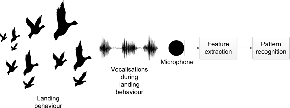
For our purpose, we identified three relevant behaviours (landing, foraging and flushing), which are all accompanied by distinct vocalisations easily identified by the human ear. The vocalisations allow us to identify a flock of geese (1) attempting to land; (2) foraging or (3) being flushed. By using vocalisation recognition, we are then able to automatically detect a flock of geese attempting to land and to assess the effect of a scaring (see Figure 1). Thereby, the concept allows us to monitor potential habituation (i.e., the situation, when geese no longer respond to scaring) and, accordingly, change our scaring strategy.
Typical methods used within animal behaviour research are based on attached tracking devices, like Global Positioning System (GPS) [4] or other wireless transmitters in a wireless sensor network [5,6], or accelerometers, measuring the movement of specific parts of the animal body [7]. Acoustic information has also been used in chewing behaviour recognition of cows [8], however these methods also rely on attaching a device on the animals. These methods are not suitable when the purpose of the animal behaviour recognition, is to utilize the results in a wildlife management system, as it is not possible to attach these devices on the animals. Vallejo and Taylor [9] uses vocalisations for source identification, based on a microphone array and thereby recognise bird behaviour, however the link between a specific vocalisation and behaviour is not found. Recognition of vocalisation, however does provide a method for behaviour recognition without the need to attach any devices on the free-living animals.
Recently, audio processing and pattern recognition methods have been used for recognition of animal vocalisations [10–13] and behaviour [14–17], in a controlled experiments or on single animals. This research within automatic vocalisation recognition has been highly influenced by methods conducted within human speech and speaker recognition. This includes feature extraction techniques, focused on cepstral features [18,19] and pattern recognition algorithms such as Hidden Markov Models (HMMs) [20,21], Gaussian Mixture Models (GMMs) [20] and Support Vector Machines (SVMs) [9,22,23].
The Mel Frequency Cepstral Coefficients (MFCC) have proven to be good features within human speech recognition, as they model the human perception of sound, and is therefore also widely used within animal vocalisation recogntion. However, animal sound perception may be different than human sound perception, and other features may be more suitable. In this paper, Greenwood Function Cepstral Coefficient (GFCC) features are used as features, to describe the vocalisations, as they, like MFCC, model the preception of sound, but can be adjusted to the hearing capabilities of different species [24].
The SVM is a supervised learning algorithm which can be used in both linear and non-linear pattern recognition problems [25]. The models are based on a structural risk minimisation principle, which improves the generalisation ability of the classifier [26]. Since the introduction of the model in the 1990s [27], the SVM has become a popular method of choice for many applications, including behaviour recognition, speaker identification and object recognition [23,28,29]. In our research, the SVM was used in a multiclass classification task to classify one of three behaviours, based on their vocalisations. The models were trained with labeled data, which were extracted from the recordings.
This paper presents a new concept for detection of animal behaviour based on its vocalisation. Methodologies developed for speech recognition have been adjusted and used to distinguish between three specific behaviours. The analytical method, described in this paper, is part of ongoing research regarding a system capable of detecting behaviour of conflict species, such as barnacle goose (Branta leucopsis), and adjust its scaring stimuli based on the detected behaviour in order to avoid habituation.
2. Materials and Methods
This section describes the chosen study species, the location of recording and the methods applied.
2.1. Study Species
We chose the Russian/Baltic population of barnacle geese as our study subject. The dramatic increase in this population over the past few decades has led to serious conflict between agriculture and geese throughout the wintering range. In Denmark, the large flocks of barnacle geese, which occur along the west coast until late spring, are causing damage to both winter cereals and pastures. Moreover, barnacle geese, like other goose species, are vocal and therefore suitable for studying the relationships between vocalisations and behaviour. Although various methods have been employed to scare barnacle geese off agricultural land, to date, no successful long-term, cost-effective scaring method has been found.
2.2. Study Site
Vest Stadil Fjord is situated on the west coast of Jutland (56°11′26.23″N, 8°7′39.07″E) surrounded by cereal fields, pastures, marsh and reed beds. Vest Stadil Fjord is an important staging and wintering area for both the Svalbard-breeding population of pink-footed geese (Anser brachyrhyncus) and the Russian-breeding barnacle geese.
The recordings took place in April 2011, when up to 10,000 barnacle geese staged in the area.
2.3. Equipment
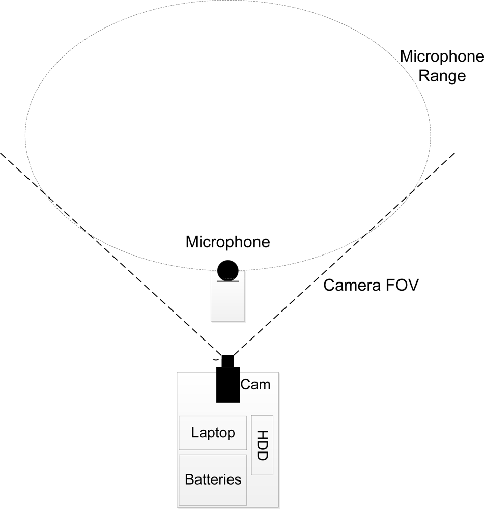
A combination of a shielded shotgun microphone (Sennheiser MKE 400) and a machine vision camera (uEye UI-1245LE-C) with a field of view (FOV) of 45° connected to a laptop were used for recordings. A multiple-shielded audio extension cable was used to minimise loss in fidelity. The camera and laptop were placed in a box at the edge of the field, whereas the microphone was placed 10 m in front of the camera, closer to the geese. The system was powered by two 12 V 92 Ah deep cycling car batteries and data were stored on 3 TB external hard drive. An overview is seen in Figure 2 (a detailed description can be found in Steen et al. [30]).
2.4. Data Collection
The vocalisations where recorded with a sample rate at 44.1 kHz. An uncompressed audio file (wave) was saved every five minutes during daylight hours.
The synchronised audio and video recordings were stored on an external hard drive for later processing. In order to capture the movements of the geese, the video stream was recorded at a frame rate of 20 frames per second.
During the study period there were two occurrences of barnacle geese, at two different dates, within the FOV of the camera. The recordings were categorised into the three behaviours of interest: landing, foraging and flushing. In Table 1, a description of the behaviours and the duration of the recordings are listed. The behaviours were observed as single events in both days, where the behaviours occoured.
The behaviours were manually labeled and observations, where the fidelity of the audio recordings were below a certain threshold, were excluded. The selected audio sequences were divided into 100 ms sequences.
The short duration of the recordings of the behaviour flushing results from the fact, that this event only covers a short time span.
2.5. Support Vector Machines
One of the most popular pattern recognition algorithms used in both human speech and animal vocalisations recognition is HMM, because of its capability to model both stochastic and temporal variations [10]. However, in the case of classification of flock behaviour, the vocalisations, produced by the flock, looses the temporal information, as multiple geese vocalise at the same time. Lately SVM models have been used in bird species recognition research [9,22], and other research working with real-world classification tasks [28,29]. SVM models are able to handle non-linear classification tasks, and they are based on structural risk minimisation principle, which improves the generalisation ability of the classifier [26]. For these reasons, the SVM has been chosen in this research.
Given n training examples {xi, yi}, i = 1 . . . n, where xi is the ith feature vector of the training set and yi ∈ {−1, 1} is the class label of the ith feature vector, the SVM model is trained to find a hyperplane Equation (1) which maximizes the margin (1/ ‖w‖) between two linearly separable labeled data sets. The hyperplane is parametrized by the weights w and the bias b.
This represents a binary classification problem, however, SVMs can also be used in multiclass problems as: one-versus-all SVMs, one-versus-one SVMs, pairwise coupling and error-correcting output code SVMs [26].
Maximizing the margin 1/ ‖w‖ is equivalent to minimizing ‖w‖2, which leads to a constrained optimization problem:
Some of the more popular kernel functions are the linear kernels, the radial basis function kernels Equation (5) and the polynomial kernels [25]. In this study, the radial basis function (RBF) is used:
The solution to the optimization problem in Equation (2) is
In this study, SVM is used for multiclass classification using the one-versus-one method. An SVM is trained for all K classes, where the kth model, constructs a hyperplane between class m and n. In our case, this means that each of the three models separates two distinct behaviours.
2.6. Acoustic Feature Extraction
The features used to describe animal vocalisation, in a recognition setting, are inspired by the research done within human speech and speaker recognition [19,20]. Here cepstral coefficients, such as the MFCC, are among the most popular [32,33].
The MFCC features are derived from the mel-scale, which is a non-linear frequency mapping adjusted to human hearing capabilities. A mel is a unit of measure of perceived pitch or frequency of a tone. In Fant [34] an approximation is given by
These features have been shown to be useful in human speech recognition [33,38], however animals do not perceive sounds equally as humans, which means that MFCC may not be useful for animal vocalisation feature extraction. In Clemins et al. [24] generalized perceptual features are introduced. The feature extraction is based on the Greenwood function [39], which assumes that sound perception is on a logarithmic scale (like the mel-scale), but that this scale differs for different species. Greenwood found this to hold true for mammals, however Adi et al. [40] use GFCC for recognition of ortolan bunting (Emberiza Hortulana) songs in Adi et al. [40]. The frequency warping function looks similar to the mel-scale warping, and the perceived frequency mapping is calculated as
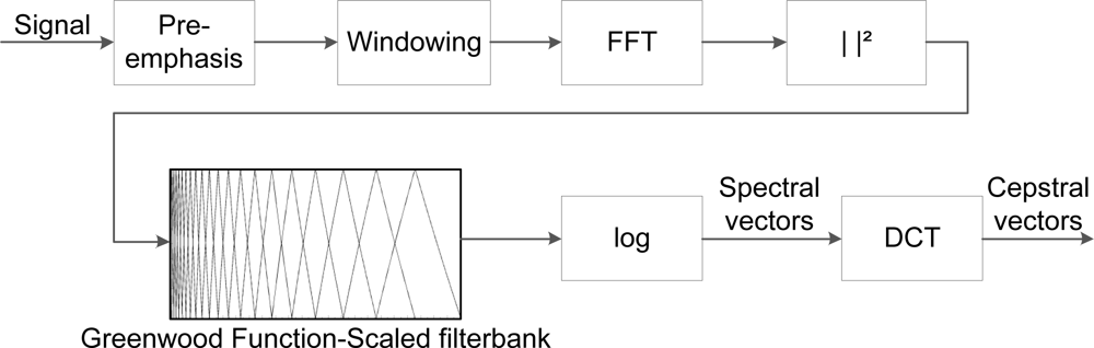
The calculation of GFCC is illustrated in Figure 3, where the incoming signal has a duration of 46 ms (2048 samples), as cepstral coefficients are derived from short-time analysis. The log-energy of each critical band is represented by spectral vectors, and a cosine transform converts the spectral vectors into cepstral vectors, according to the formula
As SVM models are based on maximizing the margin, the performance of the classifier will decrease if classes have severe overlaps. In the context of this paper, this could be the case if cepstral features does not describe the actual vocalisation, but the random background noise. These features will not provide information about the behaviour, and they could potentially cause class overlaps. Therefore feature selection has utilised to reduce the class overlap.
In this research, the feature selection selects the subset of cepstral coefficients which have the best discriminant capabilities. The feature selection is performed using the branch and bound algorithm, which finds the optimal subset of features given that the selection criterion is monotonic [26]. In this research, the sum of squared euclidian distances between features, have been used as the criterion. Using this strategy, six cepstral coefficients were chosen (cepstral coefficient number 16, 15, 5, 4, 3 and 1) and used for training and classification.
2.7. Behaviour Classification
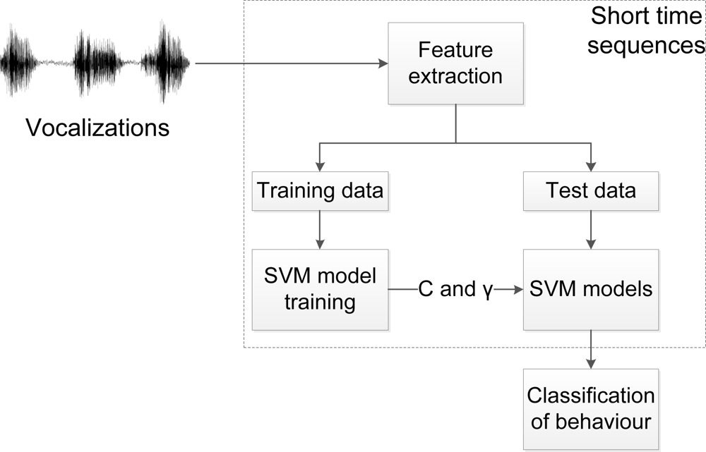
The classification of behaviour is based on the methods described in the two previous sections, and a flow describing the procedure of the behaviour classification in this research, is shown in Figure 4. The vocalisations are divided into short-time sequences, and feature extraction is performed, as shown in Figure 3. The data is divided into training and test data; whereas the SVM models are trained and utilized for behaviour classification. The behaviour classification is based on the entire audio sequence (100 ms is used in this research).
The acoustic feature extraction was performed in MATLAB R2010b, using the Voicebox toolbox [42]. The training and evaluation of the SVMs was performed using LibSVM, which is an open-source SVM toolbox supporting multiple programming languages [43].
The extracted features for the three behaviours were divided into a training data set and a test data set. There were two strategies for evaluation of classifier performance. One was to use data from day 1 as training data and data from day 2 as test data. This test strategy covers the generalisation capabilities of the classifer, as a good performance will indicate good performance on unseen data. The second test mixes all data and perform a 5-fold crossvalidation, using 4/5 as training data and the remaining 1/5 as test data. This measures the overall performance of the classifier. In the case of using day 1 as training data, the data was divided accordingly (day 1/day 2): flushing (44/56%), foraging (60/40%) and landing (62/38%), due to the distribution of the behaviours in the two days. The two strategies are named Test A and Test B, respectively.
Before training the models, the data was normalised such that all feature vectors had zero mean and unit variance Equation (12), to prevent certain features from dominating classification results due to large numerical values [26].
The training of the models consists of finding values for C and γ (as RBF kernel was chosen). This is done with a grid search, where every combination of C and γ is tested, within a predefined range or until a termination criteria is met. The evaluation of C and γ values are conducted using a five-fold cross validation scheme [44], where the C and γ with the average best cross validation rate is chosen. The grid search is done for all three SVM models, with iterative values of 2−10, 2−9, . . ., 29, 210 [44]. As more data for foraging and landing behaviour is available, the C values are scaled according to Equations (13) and (14), to compensate for this [45]
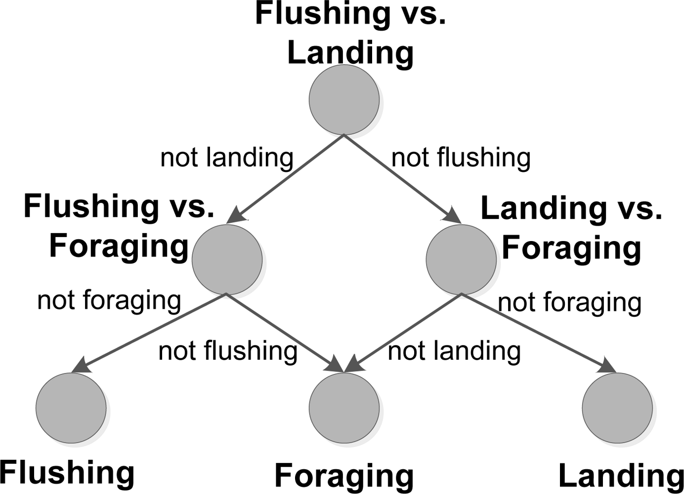
A total of three SVM models were trained, in a one-versus-one setup. The classification scheme is seen in Figure 5, where a directional graph [22,46] is used in the classification of behaviour. First the SVM model, modeling the hyperplane between flushing and landing behaviour, is evaluated and further evaluation steps are based on this result. The classification results are presented in a confusion matrix in the results section (see Table 2), which gives the number of correct positive predictions (as bold numbers) and correct negative predictions, where the classifier rejects a behaviour correctly. Positive predictions or negative predictions, which are incorrect, are also given in the table. The performance of the models are given by three measures: accuracy, precision and sensitivity.
3. Results
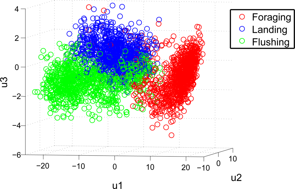
The GFCC feature extraction makes it possible to discriminate between the vocalisations of the described behaviours. This is visualised in Figure 6, where the three first principal components of the selected features, are shown. The principal components are derived via principal component analysis (PCA) [47], and are the linear combination of the selected features which preserves the most variance in a smaller dimensional space. In Figure 6, it is seen that foraging behaviour seems easiest to discriminate.
This observation is also supported in Table 3, where the overall performance of the classification is described via statistical measurements. The results in Table 3 are derived from the confusion matrix shown in Table 2, and it is seen that the overall classification performance for foraging behaviour is higher than the other two, which is visualised in Figure 6. However the overall classification performance is high, with accuracy measures over 90%. Some variability in precision and sensitivity for Test A and B is present.
The results from Test A show that the SVM models are capable of classifying unseen data, from another day, with high accuracy and precision. In this test the ratio between training and test data was close to 50/50. The results in Test B show the overall performance of the classifier. In this test, the precision was a bit lower for flushing and landing behaviour. This is expected because the vocalisations of the two behaviours are quite similar, which makes it harder for the classifier to give precise results when these behaviours are present in the audio data.
4. Discussion
The concept of using behaviour recognition in a wildlife management system requires a precise classification for the detection of goose behavior. Indeed, the results showed that acoustic measurements, feature extraction and statistical modeling may be used to classify their behaviour with a relatively high precision. Although two of the behaviours (i.e., landing and being flushed) have similarities in their vocalisations, the accuracy of classification was more than 90% for all behaviours. Therefore, by combining the three behaviors (i.e., landing, foraging, being flushed), we may obtain information sufficiently accurate for the system to respond appropriately to the presence or absence of geese in the camera FOV.
For instance, foraging behaviour was classified with a very high precision and sensitivity, which may be augmented with sequential information regarding detection of landing behaviour, as foraging behaviour would be a result of landing behaviour. However, this has yet to be investigated specifically. The detection of geese being flushed is also very important in the automatic setup, as this allows the system to verify, whether scaring has been successful or not. The performance of this detection is similar to landing behaviour, however the same argument holds, that the system could accurately use sequential information to provide a more detailed analysis on flushed behavior following a specific scaring stimulus.
In this paper, the recorded data consisted of audio and video data, although the video was only used for manual observation. To further increase classification precision, computer vision algorithms, could be to incorporated to automatically track and classify behaviour. Examples of using computer vision for this can be found in Perner [48] and Matetić et al. [49].
In this paper GFCC was used as features, and an attempt to adjust the constants to geese vocalisations has been applied. However, these are based on an approximation of the constant k, which might not be true for geese. The authors suggest an optimization based approach to derive the constants to be used, where the criteria could be discriminant analysis. This has yet to be investigated.
The concept of using vocalisation in automatic behaviour recognition could easily be incorporated in other scenarios including vocal animals. By using commercial microphones it is possible to detect the behaviour of a group of animals, as it is possible to record their intra-species communication and classify their behaviour based on the link between a certain behaviour and vocalisation. Another use, also regarding birds, could be recognition of seagul activity/harassment in cities or airports near the sea.
A complete system, capable of incorporating the automatic recognition of behaviour, is a part of ongoing research.
5. Conclusion
It is possible to distinguish between landing, foraging and flushing behaviour based on acoustic information. Landing and flushing behaviours have similarities in their vocalisations, however the accuracy for classification was over 90% for all behaviours.
The SVM modeling has proven robust, with generalisation capabilities, as results from the two test strategies are comparable. The use of GFCC as features shows promising results, however another choice of constants might prove more useful for this specific classification task.
Automatic behaviour recognition could improve automatic scaring devices, as it makes it possible to evaluate performance and alter strategies. In this paper it is shown that acoustic information can be used in the task of automatic recognition of landing, foraging and flushing behaviour.
Acknowledgments
We would like to thank Anthony D. Fox for insightful comments on the manuscript.
References
- Messmer, T.A. The emergence of human-wildlife conflict management: Turning challenges into opportunities. Int. Biodeteriro. Biodegrad 2000, 45, 97–102. [Google Scholar]
- Gilsdorf, J.M.; Hygnstrom, S.E.; Vercauteren, K.C. Use of frightening devices in wildlife damage management. Integr. Pest Manag. Rev 2002, 7, 29–45. [Google Scholar]
- Nolte, D. Behavioral Approaches For Limiting Depredation by Wild Ungulates. In Grazing Behavior of Livestock and Wildlife; Launchbaugh, K., Sanders, K., Mosley, J., Eds.; University of Idaho: Moscow, ID, USA, 1999; pp. 60–69. [Google Scholar]
- Rutter, S.M. Revista Brasileira de Zootecnia The integration of GPS, vegetation mapping and GIS. Rev. Bras. Zootec 2007, 36, 63–70. [Google Scholar]
- Nadimi, E.; Sø gaard, H.; Bak, T. ZigBee-based wireless sensor networks for classifying the behaviour of a herd of animals using classication trees. Biosyst. Eng 2008, 100, 167–176. [Google Scholar]
- Guo, Y.; Corke, P.; Poulton, G.; Wark, T.; Swain, D.; Corke, P.; Poulton, G.; Wark, T. Animal Behaviour Understanding Using Wireless Sensor Networks. Proceedings of the 2006 31st IEEE Conference on Local Computer Networks, Tampa, FL, USA, 14–16 November 2006; pp. 607–614.
- Müller, R.; Schrader, L. A new method to measure behavioural activity levels in dairy cows. Appl. Anim. Behav. Sci 2003, 83, 247–258. [Google Scholar]
- David, E.; Mark, S. Classifying cattle jaw movements: Comparing IGER behaviour recorder and acoustic techniques. Appl. Anim. Behav. Sci 2006, 98, 11–27. [Google Scholar]
- Vallejo, E.E.; Taylor, C.E. Adaptive sensor arrays for acoustic monitoring of bird behavior and diversity: Preliminary results on source identification using support vector machines. Artif. Life Robot 2010, 14, 485–488. [Google Scholar]
- Ren, Y.; Johnson, M.T.; Clemins, P.; Darre, M.; Glaeser, S.S.; Osiejuk, T.S.; Out-Nyarko, E. A framework for bioacoustic vocalization analysis using hidden markov models. Algorithms 2009, 2, 1410–1428. [Google Scholar]
- Milone, D.; Rufiner, H.; Galli, J.; Laca, E.; Cangiano, C. Computational method for segmentation and classification of ingestive sounds in sheep. Comput. Electron. Agric 2009, 65, 228–237. [Google Scholar]
- Schon, P.C.; Puppe, B.; Manteuffel, G. Linear prediction coding analysis and self-organizing feature map as tools to classify stress calls of domestic pigs (Sus scrofa). J. Acoust. Soc. Am 2001, 110, 1425–1431. [Google Scholar]
- Kogan, J.A.; Margoliash, D. Automated recognition of bird song elements from continuous recordings using dynamic time warping and hidden Markov models: A comparative study. J. Acoust. Soc. Am 1998, 103, 2185–2196. [Google Scholar]
- Thomas, R.E.; Fristrup, K.M.; Tyack, P.L. Linking the sounds of dolphins to their locations and behavior using video and multichannel acoustic recordings. J. Acoust. Soc. Am 2002, 112, 1692–1701. [Google Scholar]
- Manteuffel, G. Vocalization of farm animals as a measure of welfare. Appl. Anim. Behav. Sci 2004, 88, 163–182. [Google Scholar]
- Manteuffel, G.; Schön, P.C. Measuring pig welfare by automatic monitoring of stress calls. Bornimer Agrartech. Ber 2002, 29, 110–118. [Google Scholar]
- Moura, D.; Silva, W.; Naas, I.; Tolon, Y.; Lima, K.; Vale, M. Real time computer stress monitoring of piglets using vocalization analysis. Comput. Electron. Agric 2008, 64, 11–18. [Google Scholar]
- Reby, D.; André-Obrecht, R.; Galinier, A.; Farinas, J.; Cargnelutti, B. Cepstral coefficients and hidden Markov models reveal idiosyncratic voice characteristics in red deer (Cervus elaphus) stags. J. Acoust. Soc. Am 2006, 120, 4080–4089. [Google Scholar]
- Lee, C.; Chou, C.; Han, C.; Huang, R. Automatic recognition of animal vocalizations using averaged MFCC and linear discriminant analysis. Pattern Recogn. Lett 2006, 27, 93–101. [Google Scholar]
- Brown, J.C.; Smaragdis, P. Hidden Markov and Gaussian mixture models for automatic call classification. J. Acoust. Soc. Am 2009, 125, EL221–EL224. [Google Scholar]
- Trifa, V.M.; Kirschel, A.N.G.; Taylor, C.E.; Vallejo, E.E. Automated species recognition of antbirds in a Mexican rainforest using hidden Markov models. J. Acoust. Soc. Am 2008, 123, 2424–2431. [Google Scholar]
- Fagerlund, S. Bird species recognition using support vector machines. EURASIP J. Adv. Signal Process 2007, 2007, 1–9. [Google Scholar]
- Campbell, W.M. Speaker verification using support vector machines and high-level features. IEEE Trans. Audio Speech Lang. Process 2007, 10, 1641–2094. [Google Scholar]
- Clemins, P.; Trawicki, M.; Adi, K.; Johnson, M. Generalized Perceptual Features for Vocalization Analysis Across Multiple Species. Proceedings of the 2006 IEEE International Conference on Acoustics Speed and Signal Processing Proceedings, Toulouse, France, 14–19 May 2006; pp. I-253–I-256.
- Burges, C.J.C. A tutorial on support vector machines for pattern recognition. Data Mining Knowl. Discov 1998, 2, 121–167. [Google Scholar]
- Theodoridis, S.; Koutroumbas, K. Pattern Recognition, 4th ed; Academic Press: Waltham, MA, USA, 2008. [Google Scholar]
- Vapnik, V.N. The Nature of Statistical Learning Theory; Springer-Verlag Inc: New York, NY, USA, 1995. [Google Scholar]
- Martiskainen, P.; Järvinen, M.; Skön, J.P.; Tiirikainen, J.; Kolehmainen, M.; Mononen, J. Cow behaviour pattern recognition using a three-dimensional accelerometer and support vector machines. Appl. Anim. Behav. Sci 2009, 119, 32–38. [Google Scholar]
- Blanz, V.; Scholkopf, B.; Bultho, H.; Burges, C.; Vapnik, V.; Vetter, T. Comparison of View-Based Object Recognition Algorithms Using Realistic 3D Models. Proceedings of the International Conference on Artifiial Neural Networks, Bochum, Germany, 16–19 July 1996; pp. 251–256.
- Steen, K.A.; Karstoft, H.; Green, O. A Multimedia Capture System for Wildlife Studies. Proceedings of the Third International Conference on Emerging Network Intelligence, Lisbon, Portugal, 20–25 November 2011; Number c,. pp. 131–134.
- Cortes, C.; Vapnik, V. Support vector networks. Mach. Learn 1995, 20, 273–297. [Google Scholar]
- Bimbot, F.; Bonastre, J.F.; Fredouille, C.; Gravier, G.; Magrin-Chagnolleau, I.; Meignier, S.; Merlin, T.; Ortega-García, J.; Petrovska-Delacrétaz, D.; Reynolds, D.A. A tutorial on text-independent speaker verification. EURASIP J. Adv. Signal Process 2004, 2004, 430–451. [Google Scholar]
- Deller, J.R., Jr.; Proakis, J.G.; Hansen, J.H. Discrete Time Processing of Speech Signals, 1st ed; Prentice Hall PTR: Upper Saddle River, NJ, USA, 1993. [Google Scholar]
- Fant, C. Analysis and Synthesis of Speech Processes. In Manual of Phonetics; Malmberg, B., Ed.; North-Holland: Amsterdam, the Netherlands, 1968; pp. 173–277. [Google Scholar]
- Ganchev, T.; Fakotakis, N.; Kokkinakis, G. Comparative Evaluation of Various MFCC Implementations on the Speaker Verification Task. Proceedings of the Proceedings of Speech and Computer, Patras, Greece, 17–19 October 2005; 1, pp. 191–194.
- Dmitrieva, L.P.; Gottlieb, G. Influence of auditory experience on the development of brain stem auditory-evoked potentials in mallard duck embryos and hatchlings. Behav. Neural Biol 1994, 61, 19–28. [Google Scholar]
- Davis, S.; Mermelstein, P. Comparison of parametric representations for monosyllabic word recognition in continuosly spoken sentences. IEEE Trans. Acoust. Speech Signal Process 1980, 28, 357–366. [Google Scholar]
- Zeng, Z.; Pantic, M.; Roisman, G.I.; Huang, T.S. A survey of affect recognition methods: Audio, visual, and spontaneous expressions. IEEE Trans. Pattern Anal. Mach. Intell 2009, 31, 39–58. [Google Scholar]
- Greenwood, D.D. Critical bandwidth and consonance in relation to cochlear frequency-position coordinates. Hear. Res 1991, 54, 164–208. [Google Scholar]
- Adi, K.; Johnson, M.T.; Osiejuk, T.S. Acoustic censusing using automatic vocalization classification and identity recognition. J. Acoust. Soc. Am 2010, 127, 874–883. [Google Scholar]
- LePage, E.L. The mammalian cochlear map is optimally warped. J. Acoust. Soc. Am 2003, 114, 896–906. [Google Scholar]
- Brookes, M. VOICEBOX: Speech Processing Toolbox for MATLAB; Techinical Report; University of London: London, UK, 1997–2011; Available online: http://www.ee.ic.ac.uk/hp/staff/dmb/voicebox/voicebox (accessed on 20 March 2012). [Google Scholar]
- Chang, C.C.; Lin, C.J. LIBSVM: A library for support vector machines. ACM Trans. Intell. Syst. Technol 2011, 2, 1–27. [Google Scholar]
- Hsu, C.W.; Chang, C.C.; Lin, C.J. A Practical Guide to Support Vector Classification; Technical Report; Department of Computer Science and Information Engineering, National Taiwan University: Taipei, Taiwan, 2010; Available online: http://www.csie.ntu.edu.tw/cjlin/papers/guide/guide.pdf (accessed on 20 March 2012). [Google Scholar]
- Ben-Hur, A.; Weston, J. A User’s Guide to Support Vector Machines. Methods Mol. Biol 2008, 609, 223–239. [Google Scholar]
- Platt, J.C.; Way, M.; Shawe-Taylor, J. Large Margin DAGs for Multiclass Classification; MIT Press: Cambridge, MA, USA, 2000; pp. 547–553. [Google Scholar]
- Bishop, C.M. Pattern Recognition and Machine Learning (Information Science and Statistics); Springer-Verlag Inc: Secaucus, NJ, USA, 2006. [Google Scholar]
- Perner, P. Motion Tracking of Animals for Behavior Analysis. Proceedings of the 4th International Workshop on Visual Form (IWVF4 ’01), Capri, Italy, 28–30 May 2001; 2059/2001, pp. 779–786.
- Matetić, M.; Ribarić, S.; Ipšić, I. Qualitative modelling and analysis of animal behaviour. Appl. Intell 2004, 21, 25–44. [Google Scholar]


| Behaviour | Definition | Number of events | Duration | ||
|---|---|---|---|---|---|
| Day 1 | Day 2 | Total | |||
| Landing | Multiple geese approach the field and land on the ground | Two single events | 48 s | 30 s | 78 s |
| Foraging | Multiple geese stay on the ground and pick food from the field | Multiple events a | 90 s | 60 s | 150 s |
| Flushing | Some geese take off, and the rest of the foraging flock follow, leaving the field empty of geese | Two single events | 12 s | 15 s | 27 s |
aTwo events with high audio fidelity was selected, as the duration of foraging data should not be large compared to the other behaviours.
| Observed behaviour | Predicted behaviour | Total | ||
|---|---|---|---|---|
| Flushing | Landing | Foraging | ||
| Flushing | 129/44 | 5/10 | 16/2 | 150/56 |
| Landing | 28/10 | 219/144 | 53/4 | 300/158 |
| Foraging | 5/13 | 14/28 | 581/261 | 600/302 |
| Estimate | 162/67 | 238/182 | 650/267 | |
| Behavior | Performance | ||
|---|---|---|---|
| Accuracy a | Precision b | Sensitivity c | |
| Flushing | 0.95/0:93 | 0:80/0:66 | 0:86/0:79 |
| Landing | 0:91/0:90 | 0:92/0:79 | 0:73/0:91 |
| Foraging | 0:92/0:91 | 0:89/0:98 | 0:97/0:86 |
aRatio of correct predictions (both positive and negative) that were correct;bRatio between correct postive and incorrect postive predictions;cRatio of correct classifications (ratio between the bold numbers and total samples).
© 2012 by the authors; licensee MDPI, Basel, Switzerland This article is an open access article distributed under the terms and conditions of the Creative Commons Attribution license (http://creativecommons.org/licenses/by/3.0/).
Share and Cite
Steen, K.A.; Therkildsen, O.R.; Karstoft, H.; Green, O. A Vocal-Based Analytical Method for Goose Behaviour Recognition. Sensors 2012, 12, 3773-3788. https://doi.org/10.3390/s120303773
Steen KA, Therkildsen OR, Karstoft H, Green O. A Vocal-Based Analytical Method for Goose Behaviour Recognition. Sensors. 2012; 12(3):3773-3788. https://doi.org/10.3390/s120303773
Chicago/Turabian StyleSteen, Kim Arild, Ole Roland Therkildsen, Henrik Karstoft, and Ole Green. 2012. "A Vocal-Based Analytical Method for Goose Behaviour Recognition" Sensors 12, no. 3: 3773-3788. https://doi.org/10.3390/s120303773