Reliable Finite Frequency Filter Design for Networked Control Systems with Sensor Faults

Abstract
: This paper is concerned with the reliable finite frequency filter design for networked control systems (NCSs) subject to quantization and data missing. Taking into account quantization, possible data missing and sensor stuck faults, NCSs are modeled in the framework of discrete time-delay switched systems, and the finite frequency l2 gain is adopted for the filter design of discrete time-delay switched systems, which is converted into a set of linear matrix inequality (LMI) conditions. By the virtues of the derived conditions, a procedure of reliable filter synthesis is presented. Further, the filter gains are characterized in terms of solutions to a convex optimization problem which can be solved by using the semi-definite programme method. Finally, an example is given to illustrate the effectiveness of the proposed method.1. Introduction
In recent years, there has been a growing interest in networked control systems (NCSs), which is a class of systems in which sensors, controllers and plants are connected over the network media [1–4]. Due to their advantages such as easy installation, low cost and high utilization, the NCSs have widely applications in many application areas, such as manufacturing plants, automobiles and remote process, etc. However, these systems require novel control design to account for the presence of network in the closed loop, such as network-induced delay (see e.g., [5–8]) and packet loss (see e.g., [9,10]). Further, for the NCSs where bandwidth and energy are limited, quantization becomes indispensable. Consequently, there has been a lot of researches concerning this issue, (see e.g., [11,12]).
On the other hand, filtering problem has been playing an important role in control engineering and signal processing that has attracted constant research attention, (see e.g., [13–17] and references therein). However, it is quite common in practice that measurement outputs of a dynamic system contain incomplete observations because of the temporal sensor faults, (see e.g., [18–21] and references therein). Therefore, it is natural that the reliable filtering problem in presence of possible sensor faults has recently obtained much attention and there have been many results investigating this important issue. For example, reliable filtering problems have been thoroughly investigated in [22–24] for linear systems. As for nonlinear systems, reliable filtering problems with sensor faults have also attracted many research interests [25–27].
It should be noted that disturbances considered in those papers are all considered in full frequency domain. However, practical industry systems often employ large, complex, or lightweight structures, which include finite frequency fundamental vibration modes. Thus, it is more reasonable to design reliable filters in finite frequency domain. However, to the best of the authors' knowledge, reliable filtering problems for NCSs subject to packet loss and quantization have not been fully investigated, especially in finite frequency domain where faults occur frequently. This motivates the investigation of this work.
In response to the above discussions, in this paper, the reliable finite frequency filtering problem for NCSs subject to packet loss and quantization is investigated in finite frequency domain against sensor stuck faults. Specifically, with consideration of quantization, possible packet losses and possible sensor stuck faults, NCSs are modeled in a framework of discrete time-delay switched system. Then, the definition of finite frequency l2 gain is given and an analysis condition to capture such a performance for discrete time-delay switched system is derived. With the aid of the derived conditions, a reliable filter is designed and the conclusions are presented in terms of linear matrix inequalities (LMIs). Finally, an example is given to illustrate the effectiveness of the proposed method.
The reminder of the paper is organized as follows. The problem of system modeling for NCSs with packet losses and quantization is presented in Section 2. Section 3 provides sufficient conditions for the design of reliable filters. In Section 4, an example is given to illustrate the effectiveness of the proposed method. Finally, some conclusions are presented in Section 5.
Notations
Throughout the paper, the superscript T and −1 stand for, respectively, the transposition and the inverse of a matrix; M > 0 means that M is real symmetric and positive definite; I represents the identity matrix with compatible dimension; ‖·‖ denotes the Euclidean norm; ℙ is the probability measure; ℝ(·) denotes the expectation operator; l2 denotes the Hilbert space of square integrable functions. In block symmetric matrices or long matrix expressions, we use * to represent a term that is induced by symmetry; The sum of a square matrix A and its transposition AT is denoted by He(A):= A + AT.
2. System Model and Problem Formulation
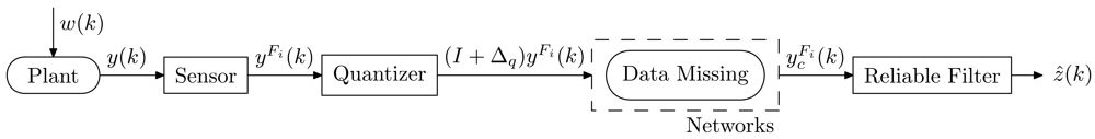
The NCS under consideration is setup in Figure 1, where the discrete-time plant is of the form:
In this paper, we make the following assumption:
Assumption 1
System (1) is stable.
Remark 2
Assumption 1 is required to get stable dynamics of the filter system. If this assumption is not satisfied, a stabilizing output feedback controller is required.
When the sensors in the NCSs experience faults, we consider the following sensor stuck fault model similar to [28],
It is also assumed that, as shown in Figure 1, the measurement signals will be quantized before transmitting via the networks wherein data missing may occur. The following logarithmic quantizer as proposed in [29] is applied,
Therefore, the faulty measurements together with quantization and the data transmission in the networks can be described by
Remark 3
The description of data transmission (8) was introduced in [30]. It can be seen that the output y(k) of the system model is (I + Δq)yFi(k) with probability δ̄ at k-th sampling time, and the value (I + Δq)yFi(k − 1) with probability 1 − δ̄ Obviously, if the binary stochastic variable α takes the value 0 consecutively at different sample times, the consecutive data missing would occur.
In this paper, the following reliable filter is constructed:
Denoting ζ(k) = [xT(k) xˆT(k)]T and e(k) = z(k) – z̃(k), then the filtering error system for the ith fault mode can be described by the following two subsystems.
S1: No packet dropout occurs.
S2: Packet dropout occurs.
where
Due to packet drop-out, the filtering error system can be seen as combined by subsystem S1 and S2, which can be lumped into the following discrete time-delay switched system:
 = {1, 2} being a piecewise constant function.
Next, we will discuss how to design the filter parameters Af, Bf and Cf. In order to formulate the problem clearly, the following definitions are first given.
Definition 4. (Asymptotical Stable)
System (10) is said to be asymptotical stable under switching signal σk, if the solution satisfies
Definition 5
Ding et al. [17] Let γ > 0 be a given constant, then the filtering error system (10) is said to have a finite-frequency l2 gain γ, if inequality
For the low-frequency range |θ| < ϑl
For the middle-frequency range ϑ1 ≤ θ ≤ ϑ2
where ϑw = (ϑ2 − ϑ1)/2.For the high-frequency range |θ| ≥ ϑh
Now, the reliable filtering problem to be addressed in this paper can be formulated as follows:
Design a stable reliable filter (9) such that, for the quantization error, possible data missing and sensor faults, the filtering error system (10) is asymptotical stable, and with a prescribed finite-frequency l2 gain γ1 from w(k) to e(k) by satisfying the following specification
Before ending this section, the following lemmas will be first given to help us to prove our main results.
Lemma 6. (Finsler's Lemma)
For x ∈ Rn,
 ∈ Rn×n,
 ∈ Rn×m, let
⊥ be any matrix such that
⊥ = 0. The following statements are equivalent:
∈ Rn×m, let
⊥ be any matrix such that
⊥ = 0. The following statements are equivalent:
xT
![Sensors 12 07975i2]() x < 0, ∀
x < 0, ∀
![Sensors 12 07975i3]() Tx = 0, x ≠ 0,
Tx = 0, x ≠ 0,![Sensors 12 07975i3]() ⊥
⊥ ![Sensors 12 07975i2]()
![Sensors 12 07975i3]() ⊥T < 0,
⊥T < 0,∃μ ∈ Rn:
![Sensors 12 07975i2]() − μ
− μ ![Sensors 12 07975i3]()
![Sensors 12 07975i3]() T < 0,
T < 0,∃
![Sensors 12 07975i4]() ∈ Rm×n:
∈ Rm×n:
![Sensors 12 07975i2]() +
+
![Sensors 12 07975i3]()
![Sensors 12 07975i4]() +
+
![Sensors 12 07975i4]() T
T ![Sensors 12 07975i3]() T < 0.
T < 0.

Lemma 7
Given the matrices Ẽ and F̃ with appropriate dimensions, then
3. Main Results
In this section, the reliable filtering problem proposed in the above section will be investigated.
Lemma 8
Consider system (10) for i = 0, 1,…,q and a given scalar γ1 < 0, then Equation (16) holds, i.e., system (10) is with a finite frequency l2 gain γ1,if there exist matrices and such that the following inequalities hold
For the low-frequency range |θw| ≤ ϑwl
For the middle-frequency range ϑ1 ≤ θw ≤ ϑ2
where ϑc = (ϑ2 + ϑ1)/2, ϑw = (ϑ2 − ϑ1)/2.For the high-frequency range |θw| ≥ ϑwh
Proof
We first consider the middle-frequency case for system (10) with ysi(k) = 0. Assume Equation (14) holds, pre- and post-multiplying it by [ξT(k) sT(k)] and its transpose, we can derive
Similarly, by choosing ϑ1:= −ϑwl, ϑ2:= ϑwl for low-frequency case and ϑ1:= ϑwh, ϑ2:= 2π − ϑwh for high-frequency case, respectively, the results for these two cases can be derived by following the same procedure of the above proof. This completes the proof.
Remark 9
Lemma 8 presents an analysis condition for finite frequency l2 gain of system (10), where less conservatism is introduced compared with the existing full frequency conditions when frequency ranges of disturbances are known.
Remark 10
The sufficient condition, which guarantees a prescribed low frequency l2 gain from ysi(k) to e(k) for system (10), can be obtained by following the same process of Lemma 8 and utilizing relevant system matrices.
3.1. Finite Frequency Performance from w(k) to e(k)
In this section, sufficient conditions to capture the finite frequency performance from w(k) to e(k) for system (10) will be derived with the aid of Lemma 8.
Theorem 11
Consider system (10) in fault free and faulty cases (i.e., i = 0, 1,…,q) for given low frequency range |θ| ≤ ϑwl, which is with a prescribed l2 gain γ1 from w(k) to e(k),i.e., the condition (16) holds if there exist a scalar ε1 > 0, matrices X, Y, N, Af, f, Cf and
Proof
It is shown, from Lemma 8, that the condition (16) can be reached if Equation (18) holds. Further, the inequality (18) can be rewritten to
Exploiting Lemma 6 and explicit null space bases calculations on Equation (26), it is easy to get that Equation (26) holds if and only if
Performing Schur's complement on Equation (27) yields to that
Remark 12
In Theorem 11, by introducing a variable W, the coupling between the Lyapunov matrices and the filter gains will be eliminated, which does not present any structural constraint.
The previous Theorem 11 presented the condition to capture the low frequency performance. Similarly, conditions for middle frequency and high frequency performance are presented in the following two corollaries.
Corollary 13
Consider system (10) in fault free and faulty cases (i.e., i = 0, 1,…,q) for given middle frequency range ϑ1 ≤ |θw| ≤ ϑ2,which is with a prescribed l2 gain γ1 from w(k) to e(k),i.e., the condition (16) holds if there exist a scalar ε1 > 0, matrices X, Y, N, Af, f, Cf and
Proof
By following the same lines of Theorem 1, it is immediate.
Corollary 14
Consider system (10) in fault-free and faulty cases (i.e., i = 0, 1,…, q) for given high frequency range |θw| ≥ ϑwh, which is with a prescribed l2 gain γ1 from w(k) to e(k),i.e., the condition (16) holds if there exist a scalar ε1 > 0,matrices X, Y, N, Af, f, Cf and
Proof
By following the same lines of Theorem 1, it is immediate.
3.2. Low Frequency Performance from ysi(k) to e(k)
In this subsection, sufficient conditions to capture the low frequency performance (17) for system (10) will be deduced.
Theorem 15
Consider system (10) in faulty cases (i.e., i = 1,…, q) for given low frequency range |θs| ≤ ϑsl, which is with a prescribed low frequency l2 gain γ2 for nonzero ysi(k),i.e., condition (17) holds, if there exist a scalar ε2 > 0, matrices X, Y, N, Af, f, Cf and
Proof
It is easily derived, from Lemma 8 and Remark 10, that the condition (17) holds if
Following the same process in Theorem 11, we first rewrite the inequality (33) to the following form,
Exploiting Lemma 6 and explicit null space bases calculations on it, we have Equation (34) is equivalent to
⊥ = [−I AκiAκdi fi] is utilized.By applying Lemma 7 on Equation (35), the inequality Equation (32) can be reached easily This proof is completed.
3.3. Stability Condition
Since Theorems 1 and 2 presented in the above section cannot guarantee the stability of the system (10), in this subsection, asymptotical stability conditions for system (10) will be presented.
Theorem 16
Consider system (10) in fault free and faulty cases (i.e., i = 0, 1,…, q), it is asymptotical stable when w(k) = 0 and ysi(k) = 0,if there exist a scalar ε3 > 0,matrices X, Y, N, Af, f, Cf and
Proof
Consider the following Lyapunov functional candidate for w(k) = 0 and ysi(k) = 0
The forward difference of the Lyapunov functional Vi(k) along the trajectories of the system (10) is given by
By following an opposite direction to the proof for Theorem 11 and exploiting Schur's complement and Lemma 7 on Equation (36), we have γκi < 0, which implies that ΔVκi(k) < 0. Therefore, from Equation (38), one can easily obtain, for a sufficiently small scalar ρ > 0 and ζ(k) ≠ 0, that
3.4. Algorithm
Based on the above analysis, a set of optimal solutions Af, f and Cf can be obtained by solving the following optimization problem for given δq:
Then the dynamic output feedback controller gains can be computed by the following equalities:
Remark 17
On the other hand, we can obtain a coarser quantizer through solving the following optimization problem for given finite-frequency l2 gains γ2 and γ2
4. Example
In this section, an application and simulations are given to illustrate the effectiveness of the proposed methods.
The utilized model is the F-404 aircraft engine described by the following state space model [31],
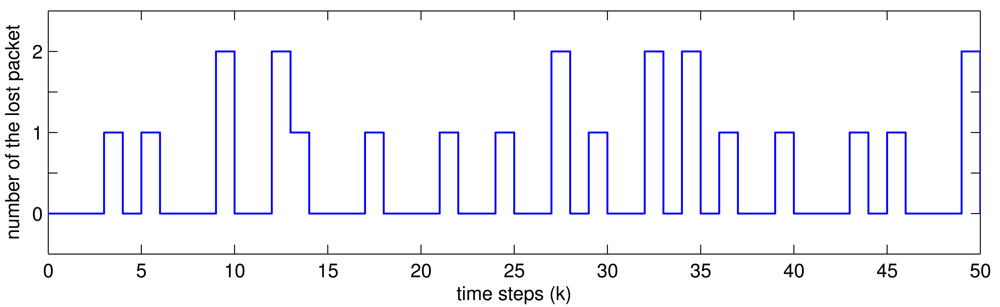
Assume the sampling period is h = 1s, and packet transmission is as shown in Figure 2, which is subject to the rate of packet lost 1 − δ̄ = 0.32.
For given ϑwl = 0.2, ϑsl = 0 and δq = 0.6, solving the optimization problem (40), we can obtain the optimal value for low frequency performances are, respectively, γ1 = 0.0825 and γ2 = 0.0378 with the corresponding reliable filter parameters
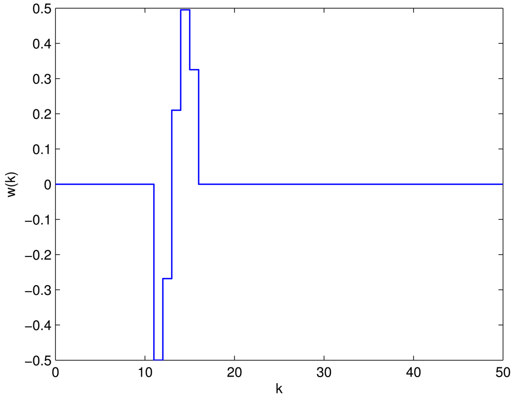
In the following, the system is simulated in low frequency domain, where the faults always occur, under the following two fault modes with zero initial condition and the disturbance input w(k) is
Mode 1
The first sensor being stuck at 0, i.e.,
Mode 2
The second sensor being stuck at 0, i.e.,
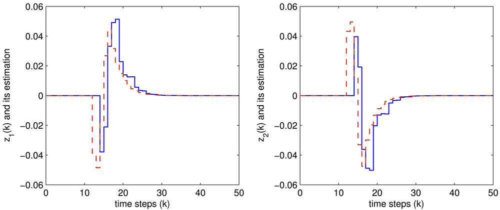
The controlled outputs and the corresponding estimations for both the two fault modes are shown in Figures 4 and 5, respectively, where the blue solid lines are the controlled output while the red dashed lines are their estimations.
It is easily seen from these figures that all the expected system performance requirement are well achieved, which shows the effectiveness of the proposed method.
5. Conclusions
In this paper, the reliable finite frequency filtering problem for NCSs subject to quantization and packet have been studied with finite frequency specifications when sensor fault would occur. The considered NCSs have been first modeled as a discrete time-delay switched system. Subsequently, a sufficient condition to characterize the finite frequency l2 gain has been presented. Then by virtues of the derived condition, a procedure of reliable filter synthesis has been derived in terms of LMIs. Finally, an example has been given to illustrated the effectiveness of the proposed method.
Acknowledgments
The authors greatly appreciate the editor, associate editor and anonymous referees for their insightful comments and suggestions that have significantly improved this article. This research has been supported by the Funds of National Science of China (Grant No. 61004061, 60975065).
References
- Dačić, D.B.; Nešić, D. Quadratic stabilization of linear networked control systems via simultaneous protocol and controller design. Automatica 2007, 43, 1145–1155. [Google Scholar]
- Yang, R.N.; Shi, P.; Liu, G.P.; Gao, H.J. Network-based feedback control for systems with mixed delays based on quantization and dropout compensation. Automatica 2011, 47, 2805–2809. [Google Scholar]
- Yang, H.J.; Xia, Y.Q.; Shi, P. Stabilization of networked control systems with nonuniform random sampling periods. Int. J. Robust Nonlinear Control 2011, 21, 501–526. [Google Scholar]
- Wang, Y.L.; Yang, G.H. Time delay and packet dropout compensation for networked control systems: A linear estimation method. Int. J. Control 2010, 81, 115–124. [Google Scholar]
- Yang, F.W.; Wang, Z.D.; Hung, Y.S. H∞ control for networked systems with random communication delays. IEEE Trans. Autom. Control 2006, 51, 511–518. [Google Scholar]
- Luan, X.L.; Shi, P.; Liu, F. Stabilization of networked control systems with random delays. IEEE Transa. Ind. Electron. 2011, 58, 4323–4330. [Google Scholar]
- Yue, D.; Han, Q.L.; Lam, J. Network-based robust H∞ control of systems with uncertainty. Automatica 2005, 41, 999–1007. [Google Scholar]
- Liu, A.D.; Yu, L.; Zhang, W.A. H∞ control for network-based systems with time-varying delay and packet disording. J. Frankl. Inst. 2011, 348, 917–932. [Google Scholar]
- Lin, H.; Antsaklis, P.J. Stability and persistent disturbance attenuation properties for a class of networked control systems: Switched system approach. Int. J. Control 2005, 78, 1447–1458. [Google Scholar]
- Xiong, J.; Lam, J. Stabilization of linear systems over networks with bounded packet loss. Automatica 2007, 43, 80–87. [Google Scholar]
- Fu, M.Y.; Xie, L.H. Finite-level quantized feedback control for linear systems. IEEE Trans. Autom. Control 2009, 54, 1165–1170. [Google Scholar]
- Fu, M.Y.; Xie, L.H. The sector bound approach to quantized feedback control. IEEE Trans. Autom. Control 2005, 50, 1698–1711. [Google Scholar]
- Basin, M.; Loukianov, A.; Hernandez-Gonzalez, M. Mean-square filtering for uncertain linear stochastic systems. Signal Process. 2010, 90, 1916–1923. [Google Scholar]
- Pan, S.; Sun, J.; Zhao, S. Robust filtering for discrete time piecewise impulsive systems. Signal Process. 2010, 90, 324–330. [Google Scholar]
- Yang, R.N.; Shi, P.; Liu, G.P. Filtering for discrete-time networked nonlinear systems with mixed random delays and packet dropouts. IEEE Trans. Autom. Control 2011, 56, 2655–2660. [Google Scholar]
- Shi, S.H.; Yuan, Z.H.; Zhang, Q.L. Fault-tolerant H∞ filter design of a class of switched systems with sensor failures. Int. J. Innov. Comput. Inf. Control 2009, 5, 3827–3838. [Google Scholar]
- Ding, D.W.; Yang, G.H. Fuzzy filter design for nonlinear systems in finite-frequency domain. IEEE Trans. Fuzzy Syst. 2010, 18, 935–945. [Google Scholar]
- Du, D.S.; Jiang, B.; Shi, P. Sensor fault estimation and compensation for time-delay switched systems. Int. J. Syst. Sci. 2012, 43, 629–640. [Google Scholar]
- Gao, Z.F.; Jiang, B.; Shi, P.; Cheng, Y.H. Sensor fault estimation and compensation for microsatellite attitude control systems. Int. J. Control Autom. Syst. 2010, 8, 228–237. [Google Scholar]
- Takahashi, M. Self-repairing control against sensor failures. Int. J. Innov. Comput. Inf. Control 2008, 4, 2919–2926. [Google Scholar]
- Cheng, Y.H.; Jiang, B.; Fu, Y.P.; Gao, Z.F. Robust observer based reliable control for satellite attitude control systems with sensor faults. Int. J. Innov. Comput. Inf. Control 2011, 7, 4149–4160. [Google Scholar]
- Liu, L.; Wang, J.; Yang, G. Reliable guaranteed variance filtering against sensor failure. Signal Process. 2003, 51, 1403–1411. [Google Scholar]
- Yang, G.H.; Ye, D. Adaptive reliable H∞ filtering against sensor failures. IEEE Trans. Signal Process. 2007, 55, 3161–3171. [Google Scholar]
- Wang, F.; Zhang, Q. LMI-based reliable H∞ filtering with sensor failure. Int. J. Innov. Comput. Inf. Control 2006, 2, 737–748. [Google Scholar]
- Guo, X.G.; Yang, G.H. Reliable H∞ filter design for discrete-time systems with sector-bounded nonlinearities: An LMI optimization. Acta Autom. Sin. 2009, 35, 1347–1351. [Google Scholar]
- Gao, H.; Zhao, Y.; Lam, J.; Chen, K. H∞ fuzzy filtering of nionlinear system with intermittent measurements. IEEE Trans. Fuzzy Syst. 2009, 17, 291–300. [Google Scholar]
- Liu, Y.S.; Wang, Z.D.; Wang, W. Reliable H∞ filtering for discrete time-delay systems with randomly occured nonlinearities via delay-partitioning method. Signal Process. 2011, 91, 713–727. [Google Scholar]
- Yang, G.H.; Wang, H. Fault detection for linear uncertain systems with sensor faults. IET Control Theory Appl. 2010, 4, 923–935. [Google Scholar]
- Elia, N.; Mitter, S.K. Stabilization of linear systems with limited information. IEEE Trans. Autom. Control 2001, 46, 1384–1400. [Google Scholar]
- Ray, A. Output feedback control under randomly carying distributed delays. J. Guid. Control Dyn. 1994, 17, 701–711. [Google Scholar]
- Li, X.J.; Yang, G.H. Fault detection for linear stochastic systems with sensor stuck faults. Optim. Control Appl. Methods 2012, 33, 61–80. [Google Scholar]


© 2012 by the authors; licensee MDPI, Basel, Switzerland. This article is an open access article distributed under the terms and conditions of the Creative Commons Attribution license (http://creativecommons.org/licenses/by/3.0/).
Share and Cite
Ju, H.-H.; Long, Y.; Wang, H. Reliable Finite Frequency Filter Design for Networked Control Systems with Sensor Faults. Sensors 2012, 12, 7975-7993. https://doi.org/10.3390/s120607975
Ju H-H, Long Y, Wang H. Reliable Finite Frequency Filter Design for Networked Control Systems with Sensor Faults. Sensors. 2012; 12(6):7975-7993. https://doi.org/10.3390/s120607975
Chicago/Turabian StyleJu, He-Hua, Yue Long, and Heng Wang. 2012. "Reliable Finite Frequency Filter Design for Networked Control Systems with Sensor Faults" Sensors 12, no. 6: 7975-7993. https://doi.org/10.3390/s120607975