Efficient k-Winner-Take-All Competitive Learning Hardware Architecture for On-Chip Learning

Abstract

A novel k-winners-take-all (k-WTA) competitive learning (CL) hardware architecture is presented for on-chip learning in this paper. The architecture is based on an efficient pipeline allowing k-WTA competition processes associated with different training vectors to be performed concurrently. The pipeline architecture employs a novel codeword swapping scheme so that neurons failing the competition for a training vector are immediately available for the competitions for the subsequent training vectors. The architecture is implemented by the field programmable gate array (FPGA). It is used as a hardware accelerator in a system on programmable chip (SOPC) for realtime on-chip learning. Experimental results show that the SOPC has significantly lower training time than that of other k-WTA CL counterparts operating with or without hardware support.

1. Introduction

The k-winners-take-all (kWTA) operation is a generalization of the winner-take-all (WTA) operation. The kWTA operation performs a selection of the k competitors whose activations are larger than the remaining input signals. It has important applications in machine learning [1], neural networks [2], image processing [3], mobile robot navigation [4] and others [5–8]. One drawback of k-WTA operations is the high computational complexities when number of input signals is large. Therefore, for realtime kWTA-based applications, hardware implementation of kWTA is usually desirable. There have been many attempts to design hardware circuits for kWTA operations. Nevertheless, many architectures are designed by analog circuits [2,9] with constraints on input signals. Because the input signals are generally not known beforehand, the circuits may not produce correct results when the constraints are not met. Although some circuits have lifted the constraints [10], overhead for the implementation of analog/digital converter is still required when the circuits are used for digital applications. In addition, some digital circuits [11–13] can only detect winners for one input set at a time. The throughput of the circuits may be further enhanced by allowing different winner detection operations sharing the same circuit at the same time.

Similar to the WTA/kWTA circuits, the winner detection is an important task in the winner-take-most (WTM) and neural gas hardware architectures. However, some hardware architectures [14,15] for WTM and neural gas networks are still based on analog circuits. Similar to the digital circuits [11–13] for WTA, the digital architecture for WTM [16] performs winner detection only for one input set at a time. The neural gas architecture [17] separates the winner detection operation into two phases: the distance computation, and sorting. These two phases are performed in an overlapping fashion. However, the sorting phase is implemented by software. Therefore, the architecture [17] may only attains limited throughput.

This paper presents a novel kWTA hardware architecture performing the concurrent winner detection operations over different input sets. The proposed architecture is suitable for digital implementation, and imposes no constraints on the input signals. To demonstrate the effectiveness of the proposed architecture, a novel kWTA-based competitive learning (CL) circuit using the proposed architecture is built. The CL algorithm has been widely used as an effective clustering technique [18,19] for sensor devices [20,21], wireless sensor networks [22,23], data approximation [24], data categorization [25] and information extraction [26]. In a CL network, the neurons compete among themselves to be activated or fired. The weight vector associated with each neuron corresponds to the center of its receptive field in the input feature space.

The CL with kWTA activation can be separated into two processes: competition and updating. Given an input training vector, the competition process finds the k best matching weight vectors to the input vector. The updating process then updates the k winners. Although existing kWTA architectures can be used for expediting the CL, these architectures only find the k winners for one input set at a time. The set of distance associated with each weight vector is used as the input set for the kWTA circuits. Different input training vectors result in different input sets. Consequently, the competition process can only be performed for one input training vector at a time. These architectures may then provide only moderate acceleration.

The proposed architecture accelerates the training process by performing the competitions associated with different input training vectors in parallel. Different input sets share the same kWTA circuit by the employment of pipeline with codeword swapping. In the proposed architecture, each training vector is allowed to carry its current k best matching neurons as it traverses through the pipeline. By incorporating the codeword swapping at each stage of the pipeline, neurons failing the competition for a training vector are then immediately available for the competitions for the subsequent training vectors. When a training vector reaches the final stage of the pipeline, a hardware-based neuron updating process is activated. The process involves the computation of learning rate and new weight vector for the winning neuron. To accelerate the process, a lookup table based circuit for finite precision division is utilized. It is able to reduce the computational time and lower the area cost at the expense of slight degradation in training process. The combination of codeword swapping scheme for neuron competition and lookup table based divider for neuron updating effectively expedites the CL training process.

The proposed architecture has a number of advantages. The first advantage of the architecture is the high throughput. Different training vectors are able to share the pipeline for the kWTA operations. The number of training vectors sharing the pipeline increases with the number of neurons. Hence, the throughput enhancement becomes very prominent as the number of neurons becomes large. An additional advantage is the low area cost. Only the comparators and multiplexers are involved in the kWTA operation. Although the tree architecture [27] is also beneficial for enhancing the throughput for the winner detection, it may need extra hardware resources. This is because the circuit needs additional intermediate nodes to build a search tree accelerating winner detection process. Each intermediate node may contain a distance computation unit, resulting in large area costs for hardware implementations.

In addition to the high throughput and low area cost, the proposed architecture can move the best k matching vectors to an input training vector to the final k stages of the pipeline, because of the employment of the codeword swapping scheme. As the number of neurons become large, after the k best matching neurons are identified, efficient retrieval of the these k winners may be complicated. By moving the winners to the final stages of the pipeline, the post-kWTA operations such as the updating process in the CL can operate directly on the final k stages of the pipeline.

To physically measure the performance, the proposed architecture has been implemented on field programmable gate array (FPGA) devices [28,29] so that it can operate in conjunction with a softcore CPU [30]. Using the reconfigurable hardware, we are then able to construct a system on programmable chip (SOPC) system for the CL clustering. In this paper, comparisons with the existing software and hardware implementations are made. Experimental results show that the proposed architecture attains a high speedup over its software counterpart for the kWTA CL training. It also has a lower latency over existing hardware architectures. Our design therefore is an effective alternative for the applications where realtime kWTA operations and/or CL training are desired.

2. The Proposed Architecture

2.1. The CL Algorithm with k-WTA Activation

Consider a CL network with N neurons. Let y_i, i = 1, …, N, be the weight vectors of the network. In the CL algorithm with k-WTA activation, given a training vector x, the squared distance D(x, y_i) between x and yⁱ is computed. The dimension of input vectors and weight vectors is 2ⁿ × 2ⁿ. Any weight vector y_i* belonging to (x) will be updated, where (x) is the set of the k best matching weight vectors to x. The updated y_i* is then given as:

$${\mathbf{\text{y}}}_{i\ast }\leftarrow {\mathbf{\text{y}}}_{i\ast }+{\eta }_{i\ast }(\mathbf{\text{x}}-{\mathbf{\text{y}}}_{i\ast })$$

(1)

where η_i* is the learning rate of the y_i*. Discovering the vector (x) requires an exhaustive search over N vectors. When N and/or n is large, the computational complexity of CL algorithm is very high.

2.2. The Architecture Overview

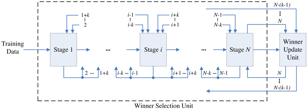
The proposed architecture is a (N + 1)-stage pipeline for a CL network with N neurons, as shown in Figure 1. The architecture can be divided into two units: winner selection unit and winner update unit. The winner selection unit includes N stages, where each stage contains one neuron in the CL network. The goal of winner selection unit is to find the set of k best matching vectors to x. The winner selection unit is therefore a kWTA circuit.

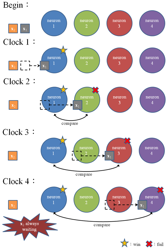
To allow multiple training vectors concurrently sharing the winner selection unit for the kWTA operation, a codeword swapping operation is adopted by the pipeline. By the employment of the codeword swapping circuit, the k best matching neurons can be traversed through the pipeline with the training vector. Figure 2 shows an example of codeword swapping scheme. For the sake of simplicity, there are only 4 neurons in the network (i.e., N = 4) with k = 1. Assume that the weight vector associated with the first neuron is closest to the current training vector x (i.e., j* = 1). As shown in Figure 2, when a training vector enters each stage, the codeword swapping circuit will be activated for that stage so that the best matching neuron can also be traversed through the pipeline with the training vector.

Without the codeword swapping scheme, the best matching neuron will always stay at the first stage, as shown in Figure 3. The subsequent training vectors are not able to enter the pipeline until the best matching neuron is updated in accordance with Equation (1). Note that the neuron updating process will be activated only when the competition at the final stage of the pipeline for the current training vector is completed. Therefore, in the case without the codeword swapping scheme, the pipeline may process only one training vector at a time. On the contrary, when the codeword swapping is employed, the neurons failing the competition will be moved forward. They will then be available for the competition for the subsequent training vectors. The proposed pipeline therefore will process the kWTA for multiple training vectors concurrently.

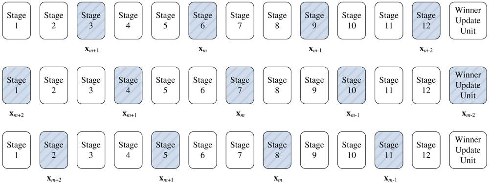
To implement the codeword swapping scheme, successive training vectors are k stages apart in the pipeline. The first k stages before a training vector x in the pipeline store the current set of k winners (x) associated with that training vector. Figure 4 gives a snapshot of the proposed architecture for k = 2. It can be observed from the figure that the pipeline allows up to ⌈(N +1)/(k + 1)⌉ competitions.

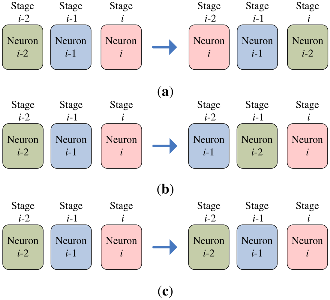
The codeword swapping operations are further elaborated in Figure 5 for k = 2. Assume a training vector x is at stage i. The current two winners associated with the x then reside at stages i − 2 and i − 1, respectively. The three neurons at stages i − 2, i − 1 and i then compete for the x. The loser will be swapped with the neuron at stage i − 2. After the swapping operations, the neuron at stage i − 2 is available for the competition for the next input vector.

The swapping operations for any k > 0 when a training vector x is currently at stage i can be extended easily. In this case, the current set of k winners (x) are located from stage i − k to stage i. The k + 1 neurons (i.e., the neurons at stages i − k, …, i) now competing for x. The worst matching neuron will then be swapped with the neuron at stage i − k.

To implement the swapping operation, each stage of the proposed pipeline architecture contains a swap unit for the implementation of swapping operations. Figure 6 shows the architecture of the swap unit at each stage i, which consists of a register and a multiplexer. The register contains y_i, the current weight vector associated with stage i. The multiplexer consists of 2k + 1 inputs: y_i−k, …, y_i+k. The k + 1 control lines c_i, …, c_i+k determine the output of the multiplexer. The c_i indicates the competition results at stage i. The c_i takes the values in the set {0, 1, …, k + 1} such that

$$c_i=\{\begin{array}{ll}0\hfill & \text{Stage}i\text{is vacant without training vector},\hfill \\ j+1\hfill & \text{A training vector}\mathbf{\text{x}}\text{is at}i,\text{and stage}i-j\text{loses competition}\hfill \end{array}$$

(2)

When x is at stage i, only stages i, i − 1, …, i − k, are involved in the competition. Therefore, 0 ≤ j ≤ k. Based on c_i defined in Equation (2), the operation of the multiplixer can be designed.

Table 1. The truth table for the multiplexer in the swap unit at stage i for k = 2.

ci	ci+1	ci+2	MUX_out	Comments
0	0	1	yi+2	x is at stage i + 2. Stage i + 2 loses competition.
0	0	2	yi+1	x is at stage i + 2. Stage i + 1 loses competition.
0	0	3	yi	x is at stage i + 2. Stage i loses competition.
0	1	0	yi	x is at stage i + 1. Stage i + 1 loses competition.
0	2	0	yi−1	x is at stage i + 1. Stage i loses competition.
0	3	0	yi	x is at stage i + 1. Stage i − 1 loses competition.
1	0	0	yi−2	x is at stage i. Stage i loses competition.
2	0	0	yi	x is at stage i. Stage i − 1 loses competition.
3	0	0	yi	x is at stage i. Stage i − 2 loses competition.
0	0	0	yi	Pipeline is in the initial state
Others			Error	Other combinations are errors.

shows the truth table of the multiplixer for k = 2. The truth table for can be easily extended for any k > 2.

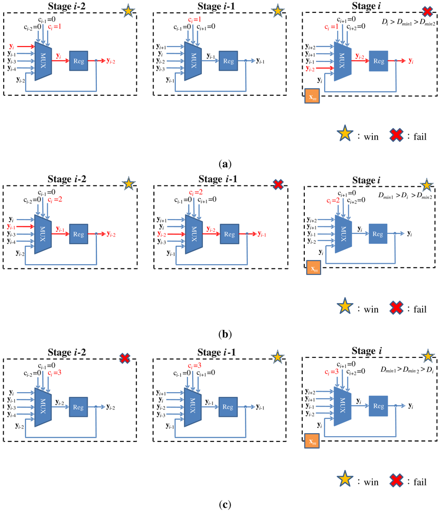
An example of the operations of swap unit is shown in Figure 7 for k = 2. In this example, assume a training vector is at stage i. Because k = 2, only the swap units at stages i, i − 1 and i − 2 are considered. Moreover, because x is at stage i, the stages i − 2, i − 1, i + 1 and i + 2 are vacant without training vector. Based on Equation (2), c_i−2 = c_i−1 = c_i+1 = c_i+2 = 0. The value of c_i will be 1, 2 or 3, dependent on the location of the neuron failing the competition. Figure 7 shows the swapping operation for each value of c_i. It can be observed from Figure 7 that with simple multiplexers, the loser will always be moved forward to stage i − 2, while the two winners are moved backward to stages i − 1 and i. In this way, the loser is available to join the competition for subsequent training vectors.

2.3. The Architecture of the Winner Selection Unit

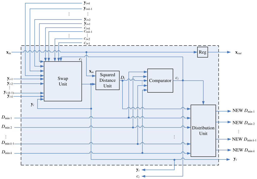
Figure 8 depicts the architecture of the stage i of the pipeline, k < i ≤ N − k, which consists of a swap unit, a squared distance unit, a comparator, and a distribution unit. Although the swap unit is the core part of the pipeline, other components are also necessary for determining the competition results c_i.

The goal of the squared distance unit is to compute D(x, y_i), the distance between the training vector x and the weight vector at stage i, where D(u, v) is the squared distance between u and v. For sake of simplicity, we let

$$D_i=D(\mathbf{\text{x}},{\mathbf{\text{y}}}_i)$$

(3)

The comparator in the architecture is used for determining the competition result c_i. As shown in Figure 8, in addition to D_i, D_minj, the squared distance between x and y_i−j, j = 1, …, k, are the inputs to the comparator, where

$$D_{{\mathit{\text{min}}}_j}=D(\mathbf{\text{x}},{\mathbf{\text{y}}}_{i-j})$$

(4)

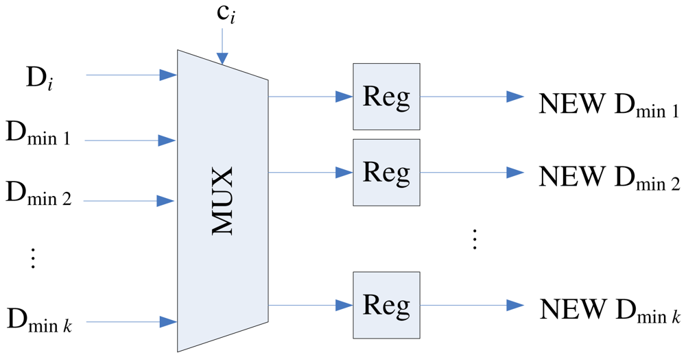
Note that the current D_min1, …, D_mink are not necessarily in ascending or descending order. After c_i at each stage i is computed, the swap unit will be activated for the codeword swapping operation. In addition, all the D_minj, j = 1, …, k, will be updated and stored in the distribution unit. The updating process should be consistent with the swapping process so that as x proceeds to the next stage (i.e., i ← i + 1), the new D_minj actually represents the squared distance between x and new y_i−j. The architecture of the distribution unit is shown in Figure 9, which contains a (k + 1) × k switch unit and registers. The switch unit has k + 1 inputs: D_i and old D_min1, …, D_mink. Based on the c_i value, the switch unit then remove one of the inputs, and re-shuffle the other k inputs to create the new D_min1, …, D_mink.

Table 2. The updating process of D_min1, …, D_mink of the distribution unit at stage i for k = 2.

ci	Neuron Failing the Competition	Updating Operation	Comments
1	Stage i	New Dmin1 ← old Dmin2	Swap between stages i and i − 2
		New Dmin2 ← old Dmin1
2	Stage i − 1	New Dmin1 ← Di	Swap between stages i − 1 and i − 2
		New Dmin2 ← old Dmin2
3	Stage i − 2	New Dmin1 ← Di	No Swapping is necessary
		New Dmin2 ← old Dmin1

shows the operations of switch unit for k = 2 at stage i. The operations for larger k values can be easily extended by analogy.

Figure 10 depicts the architecture of the stage i for 1 ≤ i ≤ k, which is the simplified version of the architecture shown in Figure 8. At the first k stages of the pipeline, because not all the vectors {y_i−k, …, y_i−1} in (x) are available as x enters these stages, no comparison to D_min1, …, D_mink is necessary. The comparator and distribution unit are removed, and the c_i is always 0 at these stages.

The architecture of stage i for N − k < i < N is depicted in Figure 11. All neurons at these stages will be delivered to the winner update unit for weight vector updating as the training vector x enters the winner update unit. In addition, updated neurons in (x) do not stay at the winner update unit. They will be sent back to stages where they come from. Therefore, as shown in Figure 11, an updated neuron from stage N + 1 is also an input vector to the swap unit. The architecture of stage N is shown in Figure 12. In the architecture, it is not necessary to update and store new D_min1, …, D_mink because the stage N is the final stage of the winner selection unit. The neuron competition is no longer necessary for the subsequent operations.

2.4. The Architecture of the Winner Update Unit

Figure 13 shows the architecture of the winner update unit. As shown in the figure, there are k weight vector update modules in the architecture. These modules are responsible for updating weight vectors obtained from the final k stages of the winner selection unit, which are the actual k winners when the training vector x enters the winner update unit.

Let y_i* ∈ C(x) be a real winner at the final k stages of the winner selection unit. Each update module computes the learning rate and updates new codeword for a y_i*, as shown in Figure 14. In the proposed architecture, the learning rate is given by

$${\eta }_{i\ast }=\frac{1}{4\times r_{i\ast }}$$

(5)

where r_i* denotes current number of times the weight vector y_i* wins the competition. The counter in the module is used for computing r_i*.

To compute the learning rate, each codeword y_i should be associated with its own r_i. When y_i−j and y_i are decided to be swapped, r_i−j and r_i will be swapped as well. For the sake of brevity, the circuit for swapping r_i−j and r_j at each stage i is not shown in Figures 8, 10, 11 and 12.

After the actual winner has been identified at the final k stages, their r_i* will be increased by 1 by the counter. The computation of learning rate involves division. In our design, a lookup table based divider is adopted for reducing the area complexity and accelerating the updating process.

2.5. The Proposed Architecture for On-Chip Learning

The proposed architecture can be employed in conjunction with the softcore processor for on-chip learning. As depicted in Figure 15, the proposed architecture is used as a custom user logic in a system-on-programmable-chip (SOPC) consisting of softcore NIOS II processor, DMA controller and SDRAM controller for controlling off-chip SDRAM memory. Figure 16 shows the operations of the SOPC for on-chip learning. From the flowchart shown in Figure 16, we see that the NIOS II processor is used only for the initialization of the proposed architecture and DMA controller, and the collection of the final training results. It does not participate in the CL training and data delivery. In fact, only the proposed architecture is responsible for CL training. The input vectors for the CL training are delivered by the DMA controller. In the SOPC system, the training vectors are stored in the SDRAM. Therefore, the DMA controller delivers training vectors from the SDRAM to the proposed architecture. After the CL training is completed, the NIOS II processor then retrieves the resulting neurons from the proposed architecture. All the operations are performed on a single FPGA chip. The on-chip learning is well-suited for applications requiring both high portability and fast computation.

3. Experimental Results

This section presents some numerical results of the proposed CL architecture. The design platform for the experiments is Altera Quartus II with SOPC Builder and NIOS II IDE. The target FPGA device for the hardware design is Altera Cyclone III EP3C120 [31]. The vector dimension of neurons is w = 2 × 2.

Table 3. The area costs of the proposed architecture for different number of stages N with various k.

N	k	LEs	Memory Bits	Embedded Multipliers
	1	5320/119088 (4 %)	0/3981312 (0 %)	72/576 (13 %)
16	2	10353/119088 (9 %)	0/3981312 (0 %)	136/576 (24 %)
	3	20512/119088 (17 %)	0/3981312 (0 %)	264/576 (46 %)
	4	40449/119088 (34 %)	0/3981312 (0 %)	520/576 (90 %)
	1	8244/119088 (7 %)	0/3981312 (0 %)	80/576 (14 %)
32	2	15892/119088 (13 %)	0/3981312 (0 %)	144/576 (25 %)
	3	31236/119088 (26 %)	0/3981312 (0 %)	272/576 (47 %)
	4	62096/119088 (52 %)	0/3981312 (0 %)	528/576 (92 %)
	1	10754/119088 (9 %)	0/3981312 (0 %)	88/576 (15 %)
64	2	21297/119088 (18 %)	0/3981312 (0 %)	152/576 (26 %)
	3	42974/119088 (36 %)	0/3981312 (0 %)	280/576 (49 %)
	4	40449/119088 (72 %)	0/3981312 (0 %)	536/576 (93 %)
	1	12398/119088 (10 %)	0/3981312 (0 %)	96/576 (17 %)
128	2	25784/119088 (22 %)	0/3981312 (0 %)	160/576 (28 %)
	3	51729/119088 (43 %)	0/3981312 (0 %)	288/576 (50 %)
	4	104121/119088(87 %)	0/3981312 (0 %)	544/576 (94 %)

shows the area costs of the proposed architecture for different number of stages N with various k. There are three different types of area cost considered in this experiment: number of logic elements (LEs), number of embedded memory bits, and the number of embedded multipliers. For example, given N = 128 and k = 4, the architecture consumes 12398 LEs, which is 87% of the LE capacity of the target FPGA device. It can be observed from the figure that the area costs grow linearly with N. Therefore, it can be effectively used for systems requiring large number of neurons N. The LE consumption also increases linearly with k for a fixed N. This is because the number of LEs of the swap unit at each stage grows with k. However, since the number of squared distance calculations is independent of k, the embedded multiplier consumption remains the same.

Performance analyses for different architectures are presented in

Table 4. Performance analyses for different architectures.

Architecture	[11]	[12]	[13]	[32]	[33]	Proposed
Area complexity	O(N3)	O(N)	O(N)	O(N)	O(N)	O(N)
Latency	O(1)	O(N)	O(Nk)	O(N)	O(N)	O(N)
Throughput	O(1)	O( $\frac{1}{N}$)	O( $\frac{1}{Nk}$)	O( $\frac{1}{N}$)	O( $\frac{m}{N}$)	O( $\frac{1}{k+1}$)
Pipeline	No	No	No	No	No	Yes
Comment				WTA only	m: # of modules

. The area complexity of an architecture is the number of comparators and/or processing elements in the circuit. The latency represents the time taken by the architecture to finish one competition. The throughput means the number of competitions completed per unit of time. It can be deduced from the table that the proposed architecture achieves a balance between speed and space. The proposed architecture also can apply to applications which perform specific operations on k targets found within the input set. As compared to architectures in [12,32] and [33] for the kNN application, the proposed architecture takes advantage of the pipeline fashion to have higher throughput even though these architectures have same latency of picking out k winners.

The proposed architecture is adopted as a hardware accelerator of a NIOS II softcore processor.

Table 5. The CPU time of the proposed hardware architecture and the hardware architecture proposed in [12] for different k and N values (in ms).

	k
	1		2		3		4
N	Proposed Arch.	Arch. in [12]	Proposed Arch.	Arch. in [12]	Proposed Arch.	Arch. in [12]	Proposed Arch.	Arch. in [12]
16	7.52619	77.3898	7.5292	81.6892	7.52917	85.9886	7.52921	90.2881
32	7.52651	140.3564	7.53012	144.4846	7.52942	148.6127	7.52947	152.7408
64	7.52715	266.2679	7.90321	270.3023	7.90315	274.3367	7.5292	278.371
128	7.52843	518.1164	7.90309	522.1019	7.529	526.0874	7.90332	530.0729

and

Table 6. The CPU time of the proposed hardware architecture and its software counterpart for different k and N values. (in ms)

	k
	1		2		3		4
N	Proposed Arch.	Software	Proposed Arch.	Software	Proposed Arch.	Software	Proposed Arch.	Software
16	7.52619	300.75	7.5292	325.70	7.52917	353.439	7.52921	377.1
32	7.52651	585.03	7.53012	614.37	7.52942	651.777	7.52947	686.23
64	7.52715	1176.22	7.90321	1190.58	7.90315	1249.32	7.5292	1308.22
128	7.52843	2340.11	7.90309	2333.72	7.529	2427.26	7.90332	2511.97

shows the CPU time of the proposed hardware architecture, its software counterpart and the hardware architecture proposed in [12] for various k and N values. The CPU time is the execution time of the processor for the CL over the entire training set. The software implementation is executed on the 2.8-GHz Pentium IV CPU with 1.5-Gbyte DDRII SDRAM. The architecture presented in [12] is also adopted as an accelerator for NIOS II softcore processor running on 50 MHz. The corresponding SOPC system is implemented in the same FPGA device Altera Cyclone III EP3C120. All implementations share the same set of training vectors with 65536 training vectors obtained from the 512 × 512 training image “Lena”.

We can see from Table 5 that the CPU time of the proposed architecture is lower than the other implementations. In fact, because of the pipeline implementation, the CPU time of the proposed architecture is almost independent of N. However, for the other implementations, the CPU time may grow linearly with N. Therefore, as N becomes large, the proposed architecture will have significantly higher speed for the CL training.

It can be noted from Table 6 that the CPU time increases with k. This is because the throughput of the proposed architecture decreases when k increases. Nevertheless, the speedup over its software counterpart is still high even for large k values.

To further illustrate the effectiveness of the proposed architecture, speedups of the proposed architecture over the software implementation and over the architecture presented in [12] are revealed in

Table 7. Speedups of the proposed architecture over its software counterpart and the architecture in [12] for different number of neurons N with various k.

	k
	1		2		3		4
N	Arch. in [12]	Software	Arch. in [12]	Software	Arch. in [12]	Software	Arch. in [12]	Software
16	10.2827	39.9605	10.8496	43.2582	11.4268	46.9426	11.9917	50.0849
32	18.6483	77.7293	19.1876	81.5766	19.7276	86.5640	20.2857	91.1392
64	35.3741	150.2637	34.2016	150.6451	34.7123	158.0787	36.9722	173.7529
128	68.8213	310.8364	66.0630	295.2921	69.8748	322.3881	67.0696	317.8373

. It is not surprising to see that the speedup increases with N. In particular, when N = 128 and k = 4, the speedup over the software implementation attains 318.

In

Table 8. Comparisons of various architectures in for clustering applications for dimension w = 2 × 2.

	Proposed Architecture (k = 2, N = 64)	Architecture in [34] (N = 64)	Architecture in [35] (N = 16)
FPGA	Altera	Altera	Altera
Devices Size of	Cyclone III EP3C120	Stratix II EP2S60	Cyclone III EP3C120
Training Set LEs/ Adaptive	65,536	64,000	60,000
Logic Modules	21,297	13,225	51,832
(ALMs) Embedded	LEs	ALMs	LEs
Multipliers/	152	288	288
DSP Blocks Embedded	Multipliers	DSP Blocks	Multipliers
Memory Bits Computation	0	8192	312,320
Time Estimated	7.90 ms	7.04 ms	22.86 ms
Power Consumption	155.50 mW	860.08 mW	137.45 mW

, we compare the proposed architecture with the architectures presented in [34,35] for clustering operations. The architectures in [34,35] are pipelined circuits for c-means and fuzzy c means algorithms, respectively. All the architectures have the same dimension w = 2 × 2. They all are used as hardware accelerators of the NIOS CPU for the computation time measurement. The area costs, computation time, and estimated power dissipation are considered in the comparisons. The power estimation is based on the PowerPlay Power Analyzer Tool provided by Altera. Note that direct comparisons of these architectures may be difficult because they are based on different algorithms. In addition, they are implemented on different FPGA devices. However, it can still be observed from the table that the proposed architecture has lower area costs as compared with the architectures in [34,35]. In addition, with larger training set and number of clusters, the architecture is able to perform the clustering with less computational time as compared with the architecture in [35]. The proposed architecture also has significantly lower power dissipation as compared with the architecture in [34]. The proposed architecture therefore has the advantages of low area costs, fast computation and low power consumption.

Table 9. Power consumption estimation of the proposed architecture (mW) for various k and N values.

	k
N	1	2	3	4
16	131.07	131.77	132.81	134.49
32	137.86	138.96	141.32	145.45
64	149.84	155.50	161.84	168.87
128	175.59	185.05	193.54	201.01

reveals the dependence of the power consumption of the proposed architecture on the k and N. It can be observed from the table that the power dissipation of the proposed architecture only slightly grows as k and/or N increase. In particular, when k = 4, eight-fold increase in N (i.e., from N = 16 to 128) leads to only 49.46% increase (i.e., from 134.49 mW to 201.01 mW) in power consumption. Alternatively, when N = 128, four-fold increase in k (i.e., from k = 1 to k = 4) results in only 14.47% increase (i.e., from 175.59 mW to 201.01 mW) in power dissipation. Therefore, the proposed circuit is able to maintain lower power dissipation even for large k and N values.

An application for clustering operations is the image coding. The neurons obtained after CL training can be used as the codewords of a vector quantizer (VQ). Because there are N neurons in a CL network, the CL-based VQ contains N codewords. An image coding technique using VQ involves the mapping of each input image block x into a codeword. For a full-search VQ, the selected codeword is the closest codeword to x. Therefore, the average mean squared error (MSE) of the VQ is defined as

$$\mathit{\text{MSE}}=\frac{1}{wt}\sum _{j=1}^{t}D({\mathbf{\text{x}}}_j,{\mathbf{\text{y}}}_{\alpha (x_j)})$$

(6)

where w is the vector dimension, t is the number of training vectors, and α() is the mapping given by

$$\alpha (\mathbf{\text{x}})=arg\underset{1\le i\le N}{min}D(\mathbf{\text{x}},{\mathbf{\text{y}}}_i)$$

(7)

In addition to MSE, another commonly used performance measure is the peak SNR (PSNR), which is defined as

$$\mathit{\text{PSNR}}=10log\frac{{255}^2}{\mathit{\text{MSE}}}$$

(8)

Table 10. Performance of the proposed architecture for image compression for N = 64 and dimensions w = 2 × 2.

Images		House	Lena
Software	MSE	150.0826	242.5662
	PSNR	26.3675 (dB)	24.2825 (dB)
Proposed Arch.	MSE	150.1482	242.6272
	PSNR	26.3656 (dB)	24.2814 (dB)

shows the performance of the proposed architecture for VQ with N = 64 and w = 2 × 2 for the two 512 × 512 test images “Houes” and “Lena.” The data set for CL training contains two 512 × 512 images “Baboo” and “Bridge.” The performance of software CL training is also included in the table for comparison purpose. It can be observed from table that only a small degradation in PSNR is observed for hardware implementation. The degradation mainly arises from the finite precision (i.e., 8-bit) fixed-point number representations and the lookup table based division adopted by the hardware. Nevertheless, the degradation is small as observed in the table. All these facts demonstrate the effectiveness of the proposed architecture.

4. Concluding Remarks

A high-speed and area-efficient pipelined architecture for kWTA operations has been proposed. With the aid of codeword swapping scheme, the system throughput soared due to the ability to perform competitions associated with different training vectors in parallel. The CPU time of the architecture is almost independent of the number of neurons N, and the architecture is able to attain high speedup over other hardware or software implementations for large N. The hardware resources are effectively saved by only involving comparators and multiplexers in the kWTA operation. The utilization of lookup table based circuit for finite precision division further reduces the computational time and lowers the area cost in learning process. The proposed architecture has no extra cost on retrieving winners after identifying the targets, which is beneficial for those applications that operations only perform on small number of targets selected from a large input set. Our numerical results demonstrate these virtues of the proposed architecture.

References

- Marinov, C.A.; Hopfield, J.J. Stable computational dynamics for a class of circuits with O(N) interconnections capable of KWTA and rank extractions. IEEE Trans. Circuit. Syst. 2005, 52, 949–959. [Google Scholar]
- Liu, Q.; Wang, J. Two k-winners-take-all networks with discontinuous activation functions. Neural Netw. 2008, 21, 406–413. [Google Scholar]
- Fish, A.; Akselrod, D.; Yadid-Pecht, O. High precision image centroid computation via an adaptive k-winner-take-all circuit in conjunction with a dynamic element matching algorithm for star tracking applications. Analog Integ. Circuit. Signal Process. 2004, 39, 251–266. [Google Scholar]
- De Souza, G.N.; Kak, A.C. Vision for mobile robot navigation: A survey. IEEE Trans. Pattern Anal. Mach. Intel. 2002, 24, 237–267. [Google Scholar]
- Iskandarani, M.Z.; Shilbayeh, N.F. Software controlled k-winner-take-all circuit for water supply management. Asia J. Inform. Technol. 2004, 3, 347–351. [Google Scholar]
- Liu, S.; Wang, J. A simplified dual neural network for quadratic programming with its KWT Aapplication. IEEE Trans. Neural Netw. 2006, 17, 1500–1510. [Google Scholar]
- Wolfe, W.J.; Mathis, D.; Anderson, C.; Rothman, J.; Gottler, M.; Brady, G.; Walker, R.; Duane, G. k-Winner networks. IEEE Trans. Neural Netw. 1991, 2, 310–315. [Google Scholar]
- Badel, S.; Schmid, A.; Leblebici, Y.A. VLSI Hamming Artificial Neural Network with k-Winner-Take-All and k-Loser-Take-All Capability. Proceedings of the nternational Joint Conference on Neural Networks IJCNN, Portland, OR, USA, July 2003; pp. 977–982.
- Hu, X.; Wang, J. An improved dual neural network for solving a class of quadratic programming problems and its k winners-take-all application. IEEE Trans. Neural Netw. 2008, 19, 2022–2031. [Google Scholar]
- Liu, Q.; Dang, C.; Cao, J. A novel recurrent neural network with one neuron and finite-time convergence for k-winners-take-all operation. IEEE Trans. Neural Netw. 2010, 21, 1140–1148. [Google Scholar]
- Hsu, T.C.; Wang, S.D. k-Winners-take-all neural net with Θ(1) time complexity. IEEE Trans. Neural Netw. 1997, 8, 1557–1561. [Google Scholar]
- Li, H.Y.; Hwang, W.J.; Yang, C.T. High speed k-Winner-take-all competitive learning in reconfigurable hardware. Lect. Note. Comput. Sci. 2009, 5579, 594–603. [Google Scholar]
- Lin, C.S.; Ou, P.; Liu, B.D. Design of k-WTA/Sorting Network Using Maskable WTA/MAX Circuit. Proceedings of the VLSI Symposium on Technology, Systems and Applications, Kyoto, Japan, 12–16 June 2001; pp. 69–72.
- Wojtyna, R. Analog Low-Voltage Low-Power CMOS Circuit for Learning Kohonen Networks on Silicon. Proceedings of the International Conference Mixed Design of Integrated Circuits and Systems, Wroclaw, Poland, 24–26 June 2010; pp. 209–214.
- Srovetta, S.; Zunino, R. Efficient training of neural gas vector quantizers with analog circuit implementation. IEEE Trans. Circuit. Syst. Anal. Digit. Signal Process. 1999, 46, 688–698. [Google Scholar]
- Dlugosz, R.; Kolasa, M.; Szulc, M. An FPGA Implementation of the Asynchronous Programmable Neighborhood Mechanism for WTM Self-Organizing Map. Proceedings of the International Conference Mixed Design of Integrated Circuits and Systems, Gliwice, Poland, 16–18 June 2011; pp. 258–263.
- Ancona, F.; Rovetta, S.; Zunino, R. Hardware Implementation of the Neural Gas. Proceedings of the International Conference on Neural Networks, Houston, TX, USA, 9–12 June 1997; pp. 991–994.
- Haykin, S. Neural Networks and Learning Machine, 3rd ed.; Pearson Education: McMaster, ON, Canada, 2009. [Google Scholar]
- Jain, A.K.; Murty, M.N.; Flynn, P.J. Data clustering: A review. ACM Comput. Surv. 1999, 31, 264–323. [Google Scholar]
- Men, H.; Liu, H.; Pan, Y.; Wang, L.; Zhang, H. Electronic nose based on an optimized competition neural network. Sensors 2011, 11, 5005–5019. [Google Scholar]
- Zakaria, A.; Shakaff, A.Y.M.; Masnan, M.J.; Saad, F.S.A.; Adom, A.H.; Ahmad, M.N.; Jaafar, M.N.; Abdullah, A.H.; Kamarudin, L.M. Improved maturity and ripeness classifications of magnifera indica cv. harumanis mangoes through sensor fusion of an electronic nose and acoustic sensor. Sensors 2012, 12, 6023–6048. [Google Scholar]
- Bokareva, T.; Bulusu, N.; Jha, S. Learning Sensor Data Characteristics in Unknown Environments. Proceedings of the Annual International Conference on Mobile and Ubiquitous Systems: Networking & Services, San Jose, CA, USA, 17–21 July 2006.
- Hortos, W.S. Unsupervised Learning in Persistent Sensing for Target Recognition by Wireless Ad Hoc Networks of Ground-Based sensors. Proceedings of the SPIE 2008, Marseille, France, 23–28 June 2008; p. 696105.
- Hofmann, T.; Buhmann, J.M. Competitive learning algorithm for robust vector quantization. IEEE Trans. Signal Process. 1998, 46, 1665–1675. [Google Scholar]
- Hwang, W.J.; Ye, B.Y.; Lin, C.T. A novel competitive learning algorithm for the parametric classification with Gaussian distributions. Pattern Recognit. Lett. 2000, 21, 375–380. [Google Scholar]
- Acciani, G.; Chiarantoni, E.; Fornarelli, G.; Vergura, S. A feature extraction unsupervised neural network for an environmental data set. Neural Netw. 2003, 16, 427–436. [Google Scholar]
- Bracco, M.; Ridella, S.; Zunino, R. Digital implementation of hierarchical vector quantization. IEEE Trans. Neural Netw. 2003, 14, 1072–1084. [Google Scholar]
- Bondalapati, K.; Prasanna, V.K. Reconfigurable computing systems. IEEE Trans. Comput. 2002, 90, 1201–1217. [Google Scholar]
- Hauck, S.; Dehon, A. Reconfigurable Computing; Morgan Kaufmann: San Francisco, CA, USA, 2008. [Google Scholar]
- NIOS II Processor Reference Handbook; Altera Corporation: San Jose, CA, USA, 2011. Availaible online: http://www.altera.com/literature/lit-nio2.jsp (accessed on 26 August 2012).
- Cyclone III Device Handbook; Altera Corporation: San Jose, CA, USA, 2012. Availaible online: http://www.altera.com/literature/lit-cyc3.jsp (accessed on 26 August, 2012).
- Aksin, D.Y. A high-precision high-resolution WTA-MAX circuit of O(N) complexity. IEEE Trans. Circuit. Sys. 2002, 49, 48–53. [Google Scholar]
- Li, H.Y.; Yeh, Y.J.; Hwang, W.J. Using wavelet transform and partial distance search to implement kNN classifier on FPGA with multiple modules. Lect. Note Computer Sci. 2007, 4633, 1105–1116. [Google Scholar]
- Hwang, W.J.; Hsu, C.C.; Li, H.Y.; Weng, S.K.; Yu, T.Y. High speed c-means clustering in reconfigurable hardware. Microprocess. Microsyst. 2010, 34, 237–246. [Google Scholar]
- Li, H.Y.; Yang, C.T.; Hwang, W.J. Efficient VLSI Architecture for Fuzzy C-Means Clustering in Reconfigurable Hardware. Proceedings of the IEEE International Conference on Frontier of Computer Science and Technology, Shanghai, China, 17–19 December 2009; pp. 168–174.