1. Introduction
The navigation of a mobile robot can be described as the problem of finding a suitable and collision-free motion between the two poses (position and orientation) of this robot, while obstacle mapping consists of using the sensing capabilities to obtain the representation of unknown obstacles in such a manner that it is useful for navigation [
1]. This work presents an alternative to solve these two problems by using a system that combines an aerial and a ground robot, using only the localization system of the terrestrial robot (UGV) and the image from a single camera on board the aerial robot (UAV).
The localization and obstacle detection techniques that are needed for ground robot navigation systems can use relative or absolute sensors. Relative sensors refers to those that are usually internal to the robot, and its measurement is given with respect to another position or state. Absolute sensors provides a measurement with respect to an external or global reference frame [
2]. The idea presented here is to provide a vision system on board the aerial robot as a relative sensor, and fuse this information with the absolute position of the ground robot in order to achieve an absolute measurement of the position of the obstacles. By doing this it is possible to obtain a mechanism of collaborative navigation and obstacle avoidance, that takes advantage of the heterogeneity of a mixed robotic system.
There are two main objectives for this system: The first is to obtain the relative distance from the UGV to any unknown obstacle surrounding it, and in that way, guarantee the safe navigation towards the goal or way-point. The second one is to obtain the absolute position of all obstacles detected during the navigation and build a map with their localization; this means having a list of the geo-referenced position of the obstacles. Some previous works have used a combination of aerial and ground robots to approach similar objectives [
3–
5], but there is no previous work that would have used only one on-board aerial camera for obstacle detection and avoidance; also, to our knowledge, no previous obstacle mapping was performed with fusion of an aerial image and the localization of the UGV.
One of the advantages of using an aerial visual navigation system is that the UGV field of view (FOV) is dynamic. This means that by controlling the UAV height and relative position, the UGV at some stage can perform a pseudo-zoom on an obstacle or any interesting object, as well as reconnaissance of areas outside the UGV's FOV. Moreover, it is also possible to identify rugged terrain, floor openings or negative obstacles, and other unexpected navigation obstructions in the UGV surrounds. This collaboration ensures the UGV's safety while it performs other inspection tasks. Finally, the system does not require previous knowledge from the environment and it can cover large navigation perimeters.
The collision-free navigation system is being developed in several phases. In the first step, the UGV and the obstacles in the robot pathway are identified by processing the aerial image, then techniques based in potential fields are applied to enable simple navigation and obstacle avoidance. After that, the proposed architecture will allow a local map to be built and obtain a geo-referenced position of the obstacle seen by the UAV. Also, each obstacle found can be memorized, and a global map with all the obstacles can be built. This will enable the system to merge reactive and deliberative methods.
The outline of this article is as follows: After this brief introduction, Section 2 reviews some related works. Section 3 introduces the addressed challenges. The techniques used to estimate the UGV's pose and the obstacle position are described in Section 4. Then, in Section 5, the UGV navigation and control systems used are explained. After that, the experiments performed and the results obtained both in simulations and with real robots are presented in Section 6. Finally, the conclusions are presented.
2. Related Work
Mobile robotic systems, both aerial and terrestrial, have been studied and developed over the years for several civil and military purposes. Some of those applications are focused on using mobile robots to help or substitute humans in tedious or dangerous tasks, as well as to survey and patrol large unstructured environments. This task is one of the objectives of the ROTOS project in which this work is framed.
In order to perform perimeter surveillance, a robot must be able to generate a trajectory to explore, or to navigate from, an initial point to a final point without colliding with other vehicles or obstacles. This autonomous navigation is one of the most ambitious issues in robotics research.
Concerning visual navigation, many reactive and deliberative navigation approaches have been presented up to now, e.g., in structured environments using white line recognition [
6], in corridor navigation using View-Sequenced Route Representation [
7], or more complex techniques combining visual localization with the extraction of valid planar region [
8], or visual and navigation techniques to perform visual navigation and obstacle avoidance [
9]. Some works integrate and fuse vision data from the UAV and UGV for best target tracking [
3], another work [
10] presents uncertainty modeling and observation–fusion approaches that produce considerable improvement in geo-location accuracy. Also, a different work [
11] presents a comparative study of several target estimation and motion-planning techniques and remarks on the importance (and the difficulty) of a single UAV at maintaining consistent view of moving targets.
By merging all those capacities and characteristics together, it is possible to develop a unique sensing and perception of a collaborative system. Work [
4] focus their work on a multi-robot system based on a vision-guide autonomy quad-rotor. They describe a way to take off, land and track over the UGV, where the UGV is equipped with two LEDs and a flat pattern in the surface. However, the quad-rotor does not provide information to the UGV about the environment. On the other hand, work [
12] presents a motion-planning and control system based on visual servoing (
i.e., the use of feedback from a camera or a network of cameras) in a UGV without cameras on board, but not specifically with a UAV. Even work [
5] proposes a hierarchy in which several UAVs with aerial cameras can be used not only to monitor, but also to command a swarm of UGVs.
Some of those studies have been tested in several different contexts, such as environment monitoring [
13], pursuit-evasion games [
14], fire detection and fighting [
15], multi-robot localization in highly cluttered urban environments [
16], de-mining [
17], and other multi-purpose collaborative tasks [
18].
4. Position Estimation
This section describes the techniques used to estimate the UGV's pose and the obstacle position. First the UGV's pose in a global coordinate frame is estimated by fusing the odometry, IMU and GPS readings using an Extended Kalman Filter (EKF), after that, another Kalman Filter is used to estimate the position of the obstacles using the results of the image processing algorithm.
4.1. Ground Robot Pose Estimation
The vehicle pose estimation problem can be defined as the calculations necessary to estimate the vehicle state based on the readings from several sensors. This problem is solved by using an EKF, which produces at time k a minimum mean squared error estimate ŝ(k ∣ k) of a state vector s(k). This estimation is the result of fusing a prediction of the state estimate ŝ(k ∣ k − 1) with an observation z(k) of the state vector s(k).
Vehicle Model
The vehicle model represents its three-dimensional pose (position and orientation). This pose can be parametrized as s = [t, ψ]T = [x, y, z, φ, θ, ψ]T, where t = [x, y, z]T are the Universal Transverse Mercator (UTM) coordinates and the relative height of the vehicle, and Ψ = [φ, θ, ψ]T are the Euler angles on the X-Y-Z axis also known as Roll, Pitch, Yaw.
In order to use an EKF to estimate the pose of the robot, it is necessary to express it as Multivariate Gaussian Distribution s ∼ N (μ, Σ). This distribution is defined by a six-element column vector μ, representing the mean values. Moreover, a six-by-six symmetric matrix Σ represents the covariance.
Now it is necessary to define a non-linear conditional probability density function f (s (k), u (k + 1)) which represents the probability of the predicted position given the current vector state s(k) and the control vector u(k + 1).
It is also very useful to define a global UGV transformation TUGV consisting of a rotation matrix R(Ψ) obtained from the Euler angles, and a translation t in the global reference frame.
Measurement Models
The vehicle pose is updated according to the readings from three different sensors: The internal odometry of the UGV, a IMU sensor and a GPS. Thus, it is necessary to create a model that links the measurements of each sensor with the global position of the mobile robot. As was done with the pose of the vehicle, the observations of the sensors need to be expressed as Gaussian Distribution; this means that they should provide a vector of mean values and a symmetrical matrix of covariances.
As it was done for the estimated UGV pose, a transformation
Ti is defined for each measurement. These transformations are:
- –
Odometry
The odometry provides a relative position and orientation constraint. To be able to use these measurements in a global reference frame, the transformation between two successive readings of the odometry (Todom−read(k) → Todom−read(k+1)) is calculated, and the resulting transformation is applied to the previous estimated position of the UGV.
- –
GPS.
The readings from the GPS are converted to UTM using the equations form
USGS Bulletin 1532 [
19], and they are used to provide a global position constraint. However, the GPS does not provide information for the orientation of the robot, so only the position should be taken into account.
- –
IMU.
The IMU readings are pre-processed to fuse the gyroscopes, accelerometers and magnetometers. In order to provide a global constraint of the orientation of the UGV, no position or translation constraints are obtained from this sensor.
With the transformations defined, it is possible to define a probability density function for each one of them. In all cases, the H matrix (necessary to compute the estimation of the EKF) will be an identity matrix of dimension six. For the GPS and the IMU, the covariance associated with the rotation or translation, which are not provided, will be replaced by very high values.
These models and the Kalman Filter itself are implemented using the Bayesian Filter Library [
20], which is fully integrated in the ROS environment. The estimated pose is updated at a pre-defined frequency with the data available at that time; this is an estimation of the pose to be made even if one sensor stops sending information. Also, if the information is received after a time-out, it is disregarded.
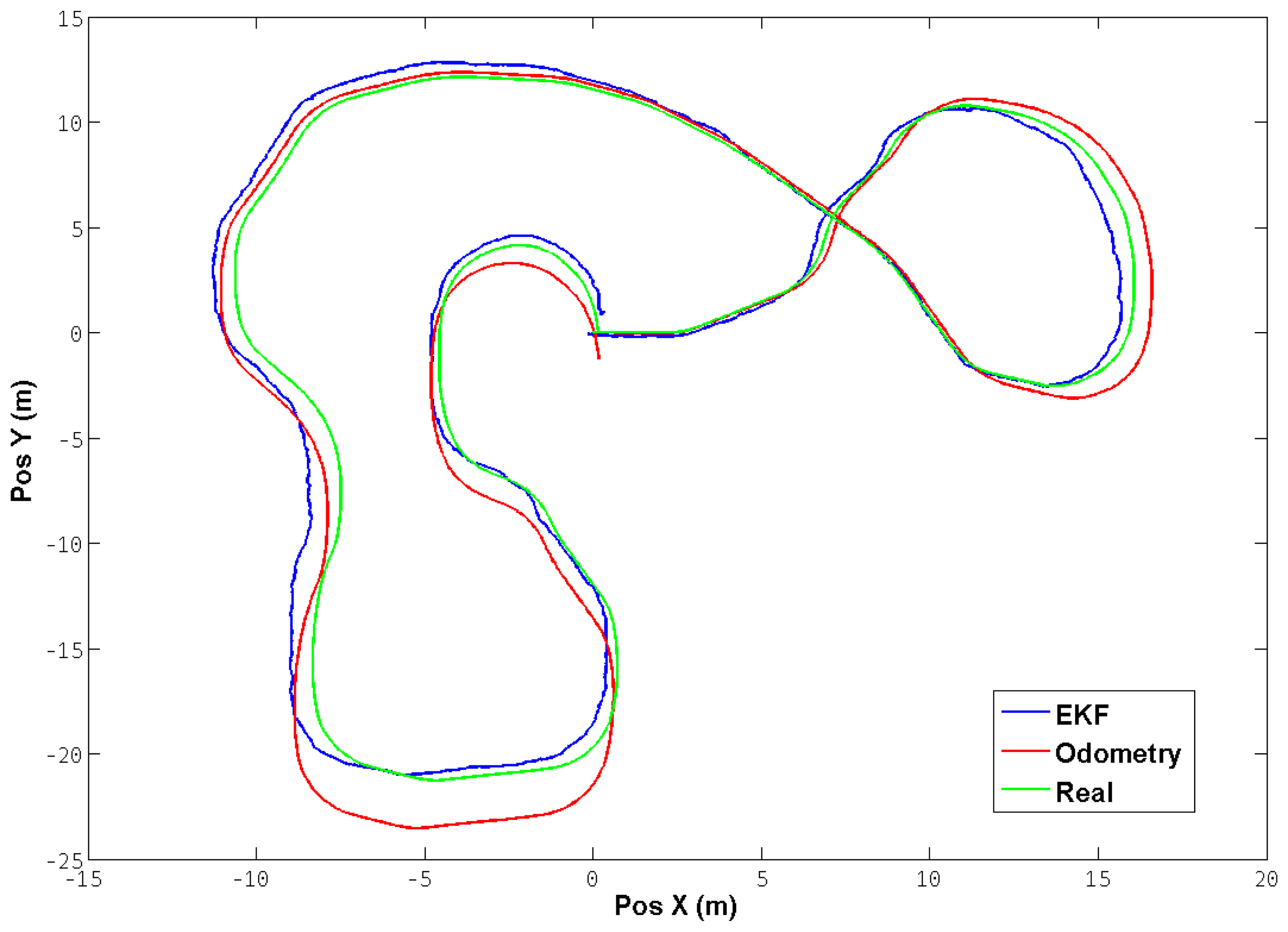
Figure 4 shows a test trajectory performed with the robot in a simulated environment. The positions were translated to a common reference frame in order to be able to compare them. It can be observed that the EKF performs a correction of the position from the odometry, thereby reducing the mean square error in comparison with the real position obtained directly from the simulator.
5. Navigation and Control
This section describes the algorithms and control laws used for the navigation of both the ground and aerial robots. Since this work is not oriented to find new control theories, a well-studied potential fields navigation is used to control the ground robot, and the aerial robot works in teleoperated mode.
5.1. Aerial Robot
The main objective of the aerial robot is to have the ground robot and as much as possible of its pathway in the field of view of its downward camera. This is assured by involving a human pilot who controls the air robot in teleoperated mode. However, there is a mid-level control system working to facilitate the operation of the air robot. The mid-level control system provides a height control based on the readings of a ultra sound range meter, it also provides a pose stabilization algorithm that attempts to keep the robot as steady as possible in order to obtain a better image, this stabilization technique is based on a fusion of optical flow and IMU readings. Since the dynamics of the aerial robot are much faster than the ground robot, there are several time lapses where the aerial robot is hovering; in those moments, the stabilization algorithm proves its utility.
Alternatively, it is possible to control the aerial robot using a ground control station (GCS) that receives the telemetry and images from the quad-rotor, before using a position control algorithm to maintain the target (UGV) in the center of the image, and sending commands to control the aerial robot flight motions (Roll
ψ and Pitch
θ angles). These control commands are sent to the aerial robot usually 30 times per second to obtain smooth movements. Additionally, the GCS is used for configuring and monitoring the aerial robot (see [
21] for a detailed architecture).
5.2. Ground Robot
The ground robot is controlled by using a ROS implementation of the Steering Behaviors [
22]. This potential fields navigation technique is based on the definition of a simple vehicle model, which is a point mass approximation. The vehicle is described by its position, orientation and velocity. Its velocity is modified by applying forces or accelerations that are limited by a maximum force parameter. This allows for a simple computational model to operate and is independent from the locomotion schema.
The pose of the vehicle is defined by four vectors, the first one is for the position of the robot, and the other three are ortho-normal vectors that define orientation (Forward, Side and Up), having the X axis as the normalized direction of the velocity or Forward vector. Since only planar movement is considered the Z axis will be constant, and the Y will be the cross product of X and Z (or Forward and Up). The control signal obtained from the algorithm is one vector that represents the steering force resulting from all the behaviors (i.e., evasion, seeking, alignment). This vector is added to the current velocity and then is mapped in order to be translated to the vehicle reference frame. It is subsequently converted into two control signals—linear and angular velocity—that are sent to the ground robot control system.
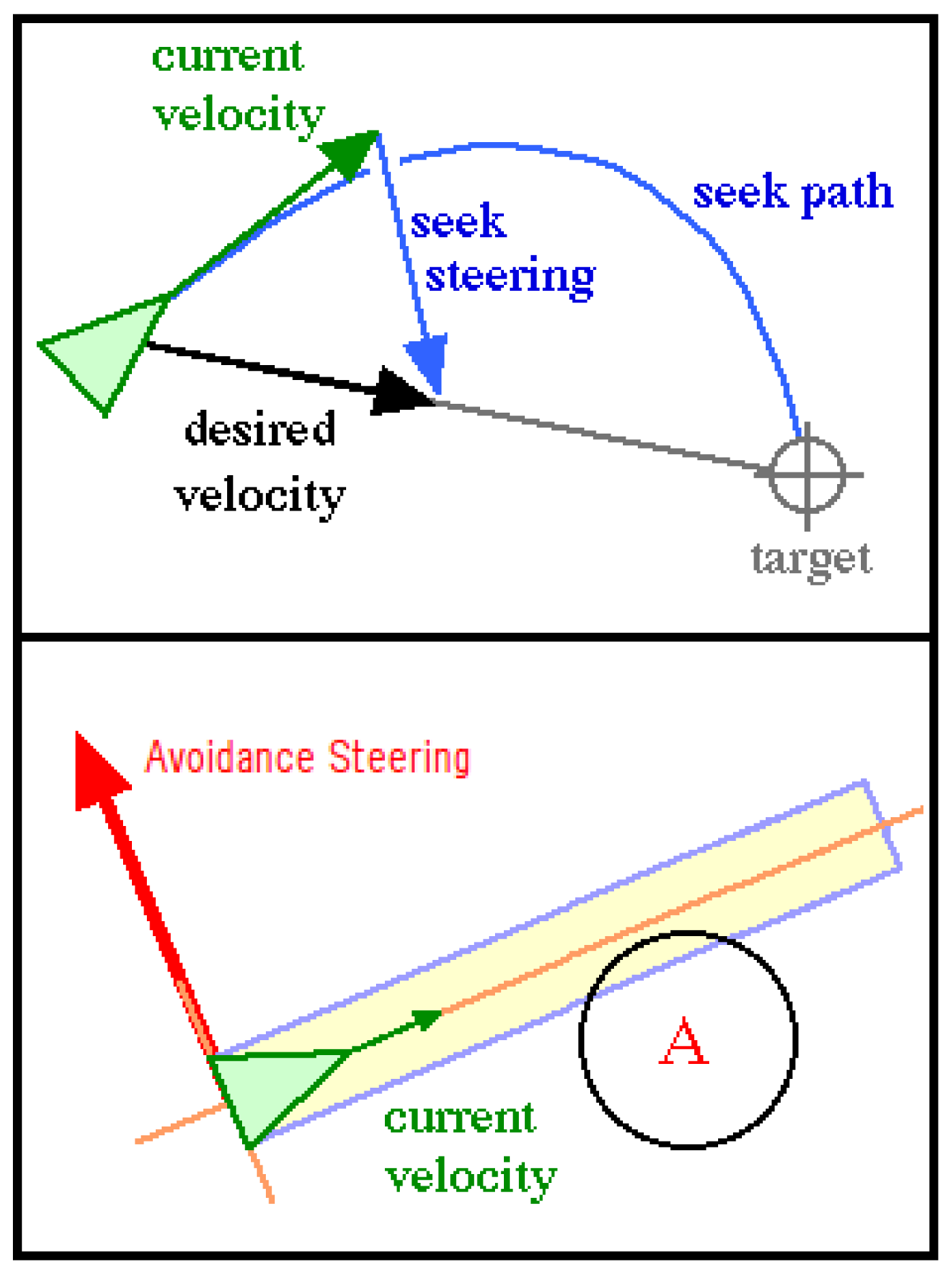
The use of the steering behaviors library for the navigation of the UGV has two main advantages: it allows the implementation of several behaviors for a single UGV or a set of them, and it is possible to dynamically add or remove obstacles, which is very convenient in this case. For this initial effort, three steering behaviors were implemented: one for seeking the target point, another for arriving at it, and the third one to avoid obstacles.
The seeking behavior tries to steer the vehicle towards a pre-defined position in the global coordinate system. The behavior adjusts the UGV velocity so it is aligned towards the target; the desired velocity is a vector defined from the vehicle position to the target at the maximum speed, and the steering vector is the difference between this desired velocity and the UGV current velocity. If only seeking behavior is used, the UGV will pass through the target and then turn back. The arriving behavior is similar to the seeking, but it implements a braking force when the vehicle is within a pre-defined distance to the target, thus making the UGV stop when it arrives at it.
Figure 5 shows the Seek and Avoid behaviors, with their resulting steering vectors and the auxiliar items used to calculate them.
The avoidance behavior is intended to provide the vehicle with the ability to maneuver in an environment where obstacles may appear; it takes action only when an obstacle is detected in front to the UGV, meaning that if it is moving parallel to a wall, the avoidance will take no action. The basic algorithm assumes that both the vehicle and the obstacles are spheres, although variations can be made to take into account the shape, and then extends the bounding sphere of the UGV to create an imaginary cylinder lying along the forward axis of the UGV, the length of the cylinder depends on the speed of the vehicle and its ability to steer. The algorithm then calculates if any of the given obstacles intersect with the UGV's cylinder. If there is no collision, a zero vector is returned; if a collision is found, the center of the obstacle is projected on the side axis of the vehicle and a steer in the opposite direction is generated. If two or more obstacles are found, the one nearest to the vehicle prevails over the rest. The two behaviors (seek and avoid) can be combined by adding the steering forces resulting for each one. It is also possible to give more priority to one or another by performing a weighted addition.
6. Experiments
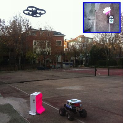
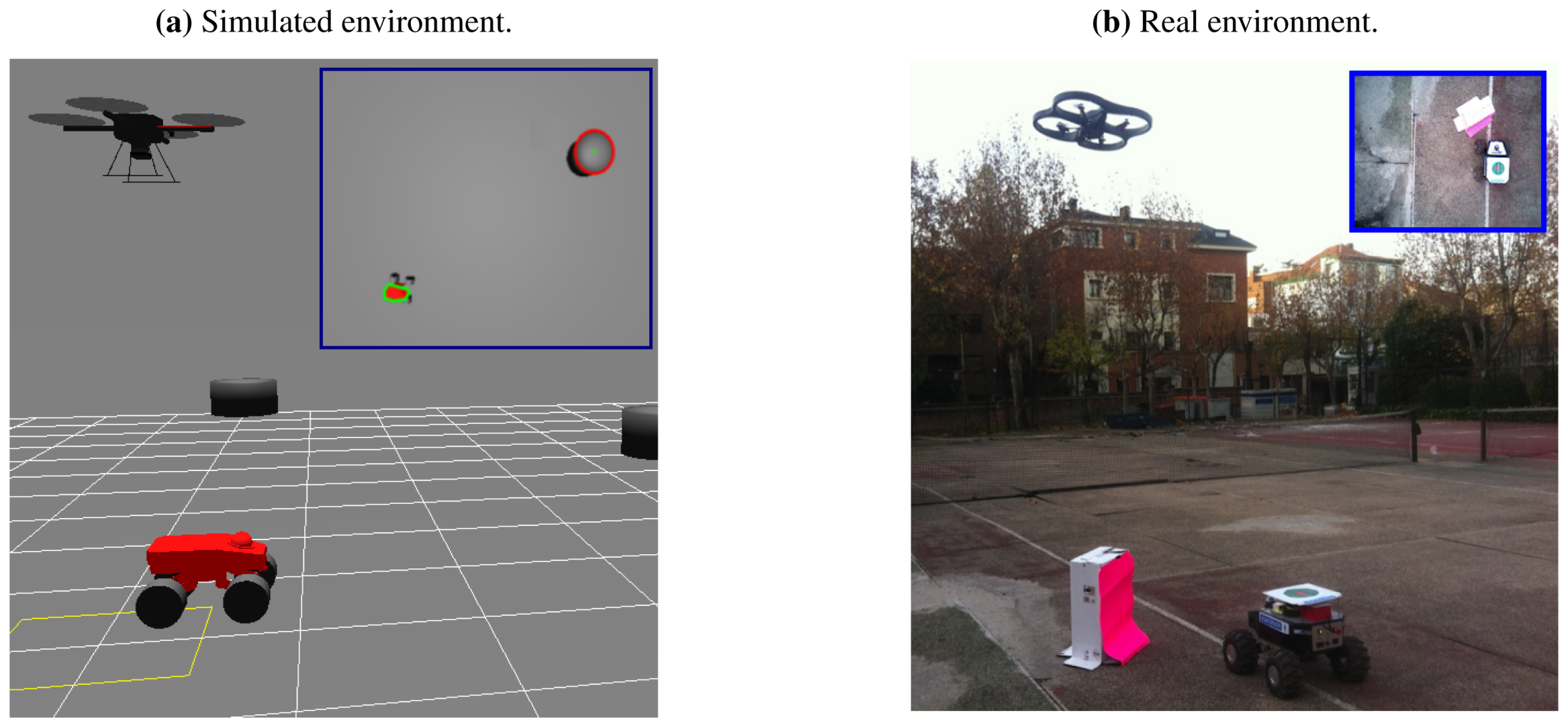
This section presents the results obtained with the proposed aerial–ground system. The approaches described in the previous sections have been implemented first on a simulation environment, and then with real robots. The software architecture used allows to use the same implementation in both environments, but it was necessary to use a realistic simulation of the entire system. First, a quad-rotor aerial robot model was used, as well as a skid-steering ground robot. Also, the sensors simulations that include typical error sources were added to the both robot models, as well as the camera model on board the UAV. By doing this, we ensure that the simulations and the real results are consistent, and that the algorithms can be translated to the real robots. The simulated and real environments are shown in
Figure 6.
6.1. Simulations
Two main tests have been performed on the simulated environment. The first one consists of a single obstacle detection and avoidance maneuver, it is done to check each part of the solution proposed, and thus validate it.
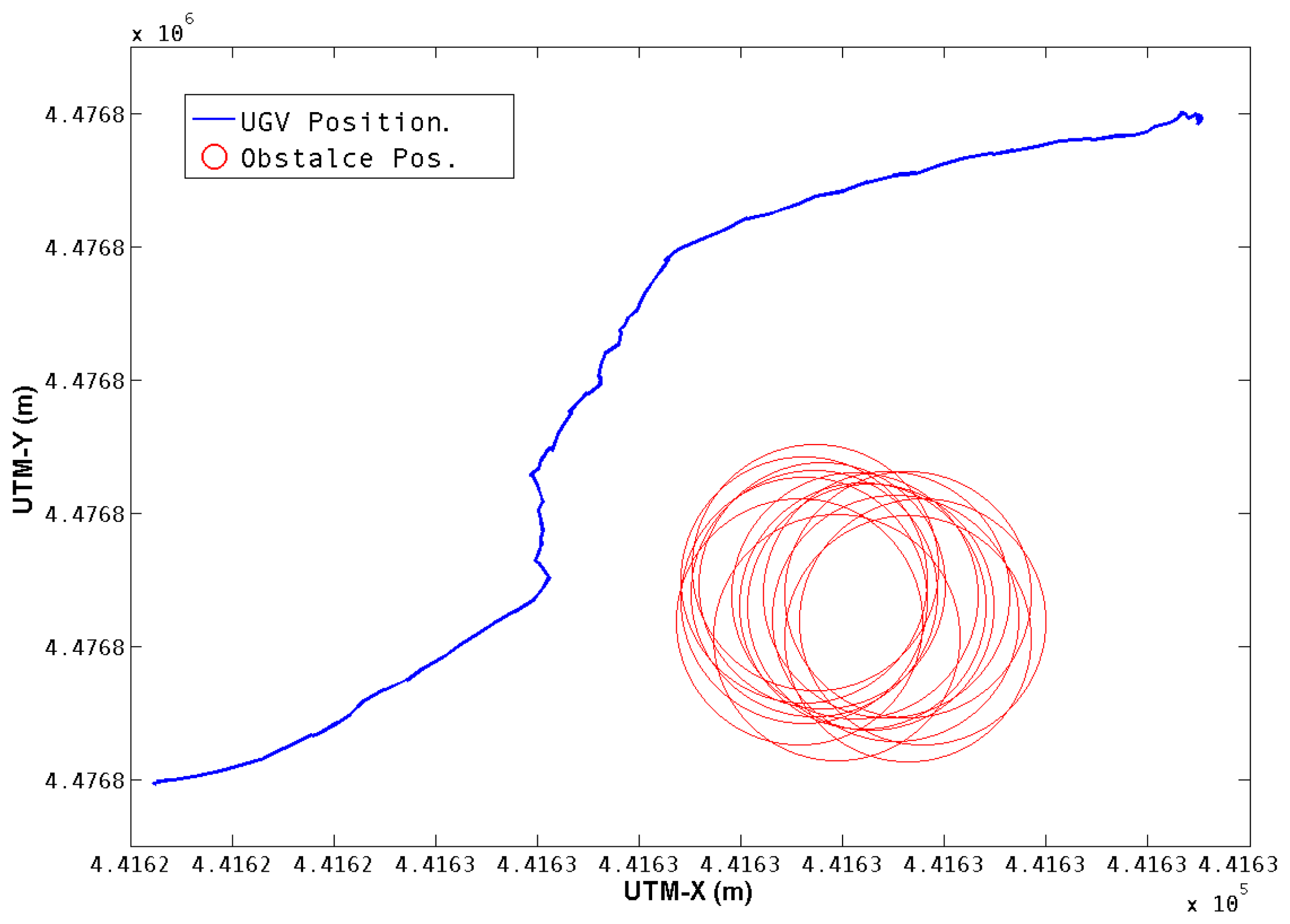
Figure 7 shows the trajectory performed for the first test. The position of the UGV in UTMs is obtained from the Extended Kalman Filter. The position of the obstacle is calculated from the aerial image and the corresponding transformations, as was described in Section 3. The total distance covered was 16.9 meters and was executed in 25 seconds.
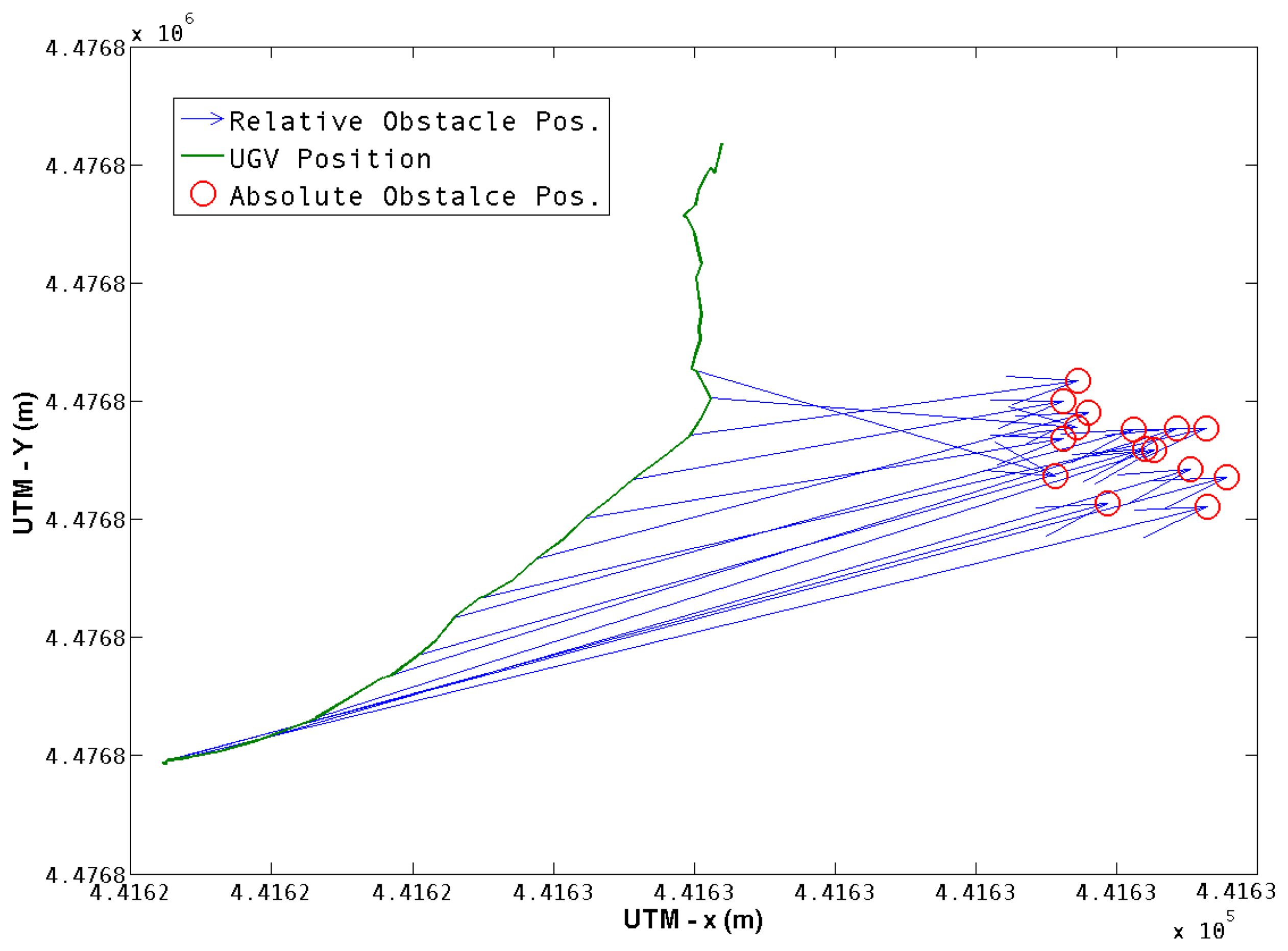
Figure 8 shows how each position was obtained, a transformation from the UGV position to the obstacle position is obtained according to
Equation (4) and is represented by blue arrows. The resulting obstacle position in the world coordinate frame is represented by red circles. Once the obstacle is left behind, its position is no longer of interest, nor is it taken into account. It can be observed that there is a dispersal of the observations of the obstacle position, so it is of interest to have a characterization of the resulting positions of the obstacle.
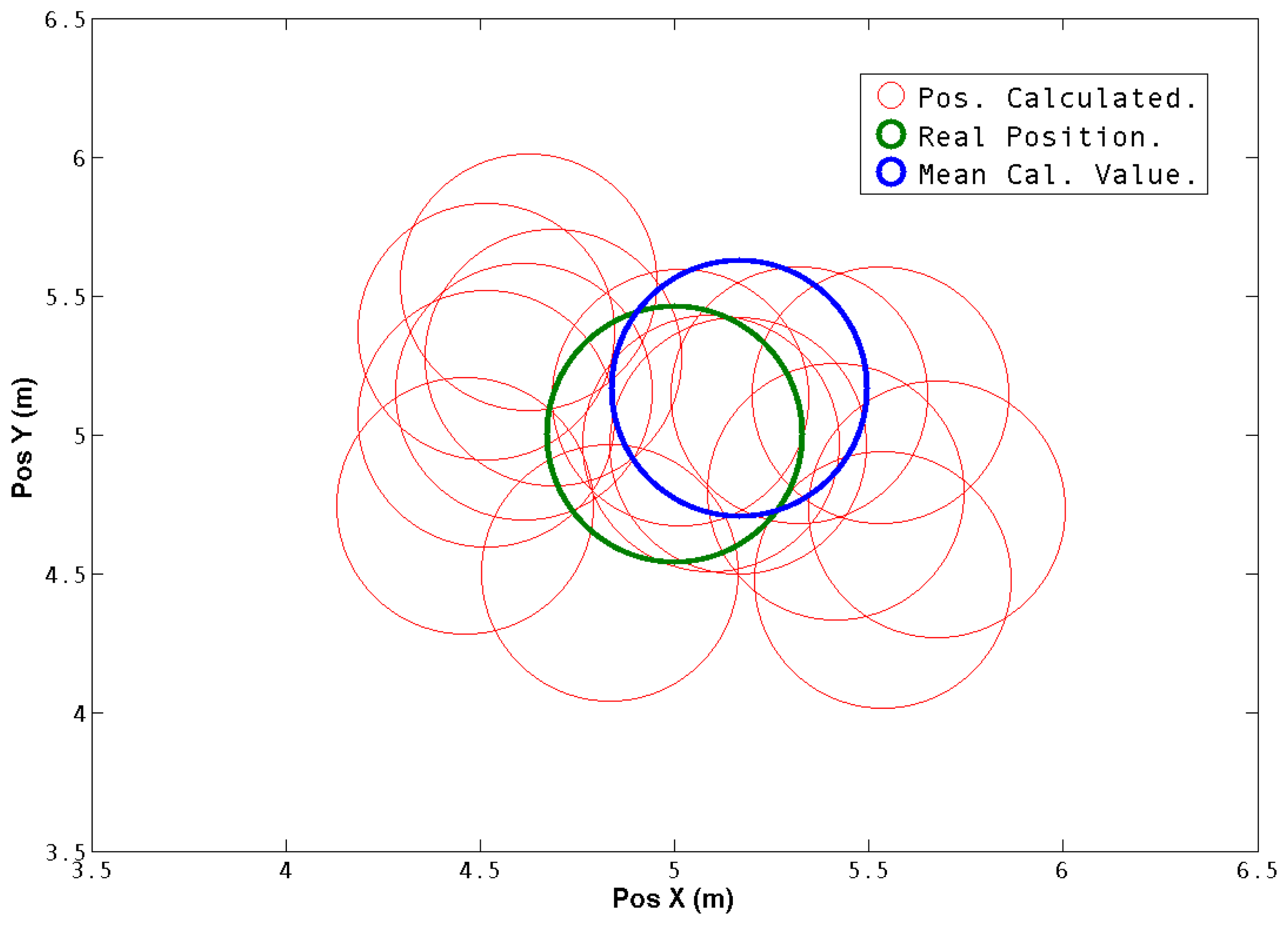
In
Figure 9 the real obstacle position and the positions obtained with the system are translated to a common reference frame and compared. The mean square error and the standard deviation were calculated and are shown in
Table 1. It is possible to see that both values are in good error ranges. The mean square error is less than 20% of the diameter of the obstacle, which is 1 meter, in the
X axis and 30% on the
Y axis.
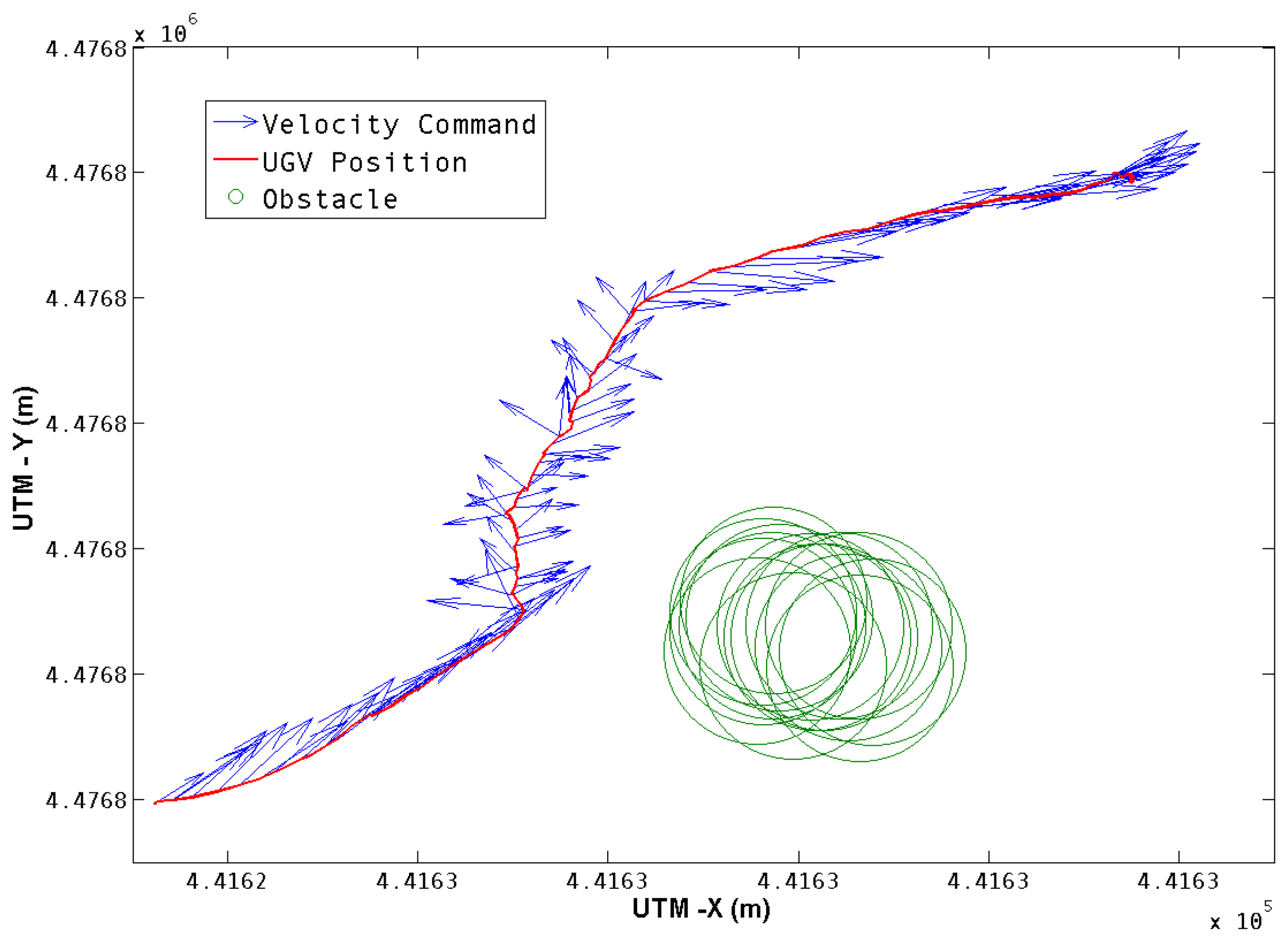
Once the obstacle position is obtained, the navigation algorithm uses this information to perform the avoidance maneuver according to the seek and avoid behaviors described in Section 5.2. The outcome of this navigation algorithm is the velocity command in each time step. The command is translated to the UGV reference frame, converted to linear and angular velocity, and sent to the robot's control system.
Figure 10 shows the velocity commands generated for this test, together with the UGV's trajectory and the obstacle position.
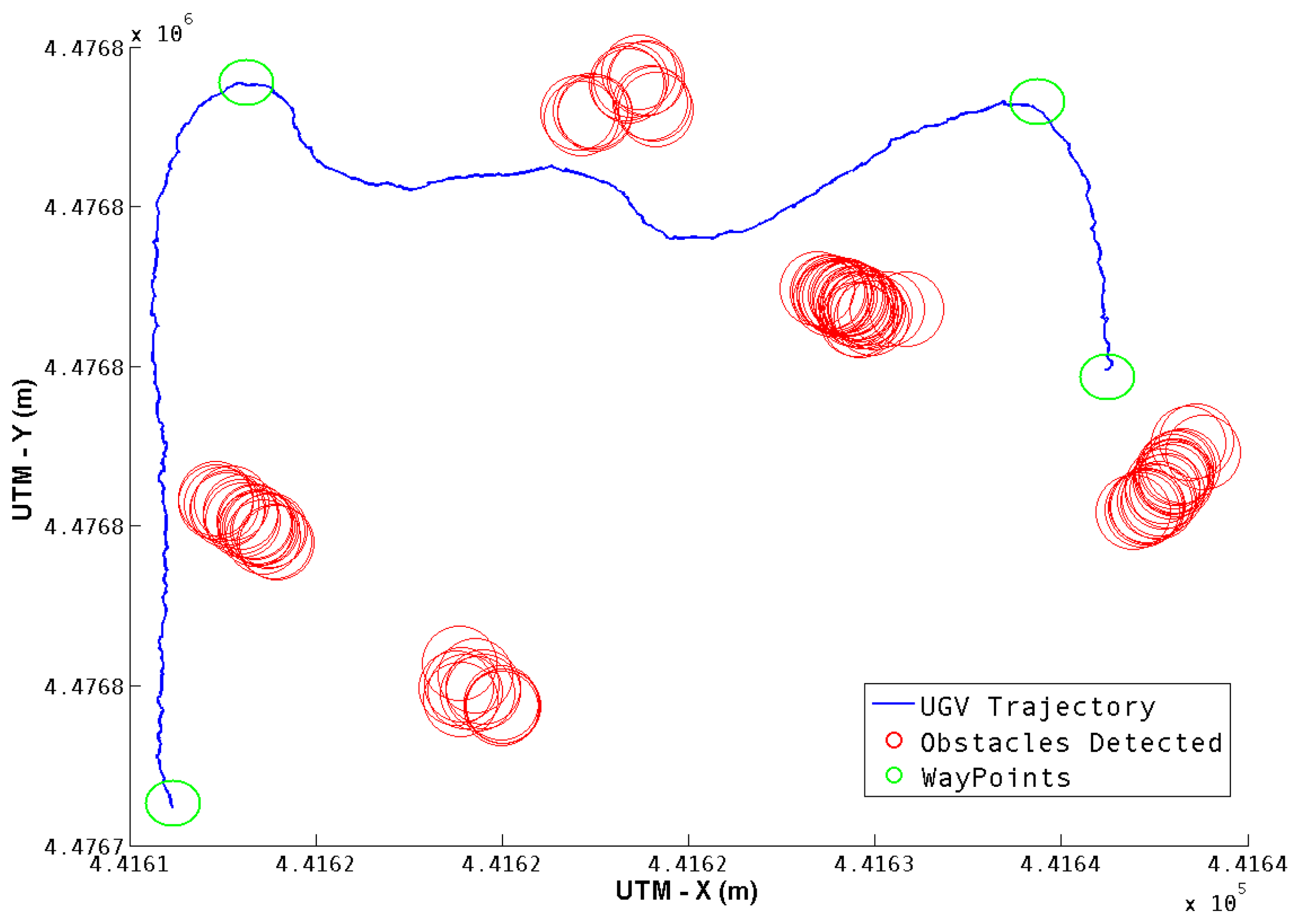
For the second test, three way-points were defined, in an environment with six cylindrical obstacles. While visiting the way-points, some obstacles were detected, and the corresponding avoidance was executed if necessary.
Figure 11 shows the full trajectory, as well as the obstacles detected. Five of the six obstacles were detected, and all three way-points were reached successfully.
The position is given in UTM coordinates, as was explained in Section 4.2. Since the values obtained for the standard deviation are in all cases less than one meter, it can be concluded that this data gives a set of obstacle positions can be used for the navigation system.
Table 2 shows the mean value and standard deviation of the five obstacles detected during the test.
6.2. Real Environment
A set of tests were designed and implemented in order to check the feasibility of the system outside of the simulated environment. The first test was oriented to check the inter-process communications. Therefore, a set of hovering flights were performed and data both from the UGV and the UAV was acquired in real-time using the middle-ware and software architecture developed for this system [
21].
The second test was carried out in an outdoor environment. Its objectives was to obtain real images from the UAV and test the feature extraction algorithms. To facilitate the tests, a platform with a geometric shape pattern was shipped in the UGV. The platform designed have two main capabilities: it can be used for take-off and emergency landings, and it can also transport the UAV in case it ran out of battery. An additional advantage is that the platform design made it easier to track the UGV and distinguish it from other features on the ground. Finally, the navigation algorithm for the UGV was tested using a fixed target and a virtual obstacle position. A set of images from those previous tests are shown in
Figure 12.
During the tests described previously, the image acquisition rate and processing times, likewise the telemetry data from both the UGV and the UAV, were tested and measured. At last, all the data processing and the commands sent to the navigation system were also measured in terms of its time period. The results of all those measurements are shown in
Table 3.
It can be observed that the image streaming runs with an average frequency of 10Hz, and that all the other times or frequencies are faster than that value. In accordance with the software architecture (defined in [
21]), the UGV's control and navigation systems run in the UGV on-board computer, and the image acquisition and processing is done on the base-station PC. Also, the inter-process communication core is handled by the ROS middle-ware framework, which enables the system to work at the same frequency as the image streaming. The results from those previous tests shown that the communications and image processing algorithms are feasible enough to perform obstacle-free navigation in real time.
In order to accomplish the last experiment with the full aerial–ground system. A set of obstacles were placed in different positions of the robot workspace. Then, a set of pre-defined and fixed targets were given to the UGV ensuring that to arrive there it must avoid the obstacles previously defined.
The obstacle-avoidance maneuver was executed using the steering behaviors algorithm. The UAV was manually controlled in hovering mode over the UGV, and images from the aerial vehicle were acquired and processed using the feature extraction algorithm. The position of the UGV and the obstacle were extracted from the image and the information of the obstacles position sent to the UGV navigation system.
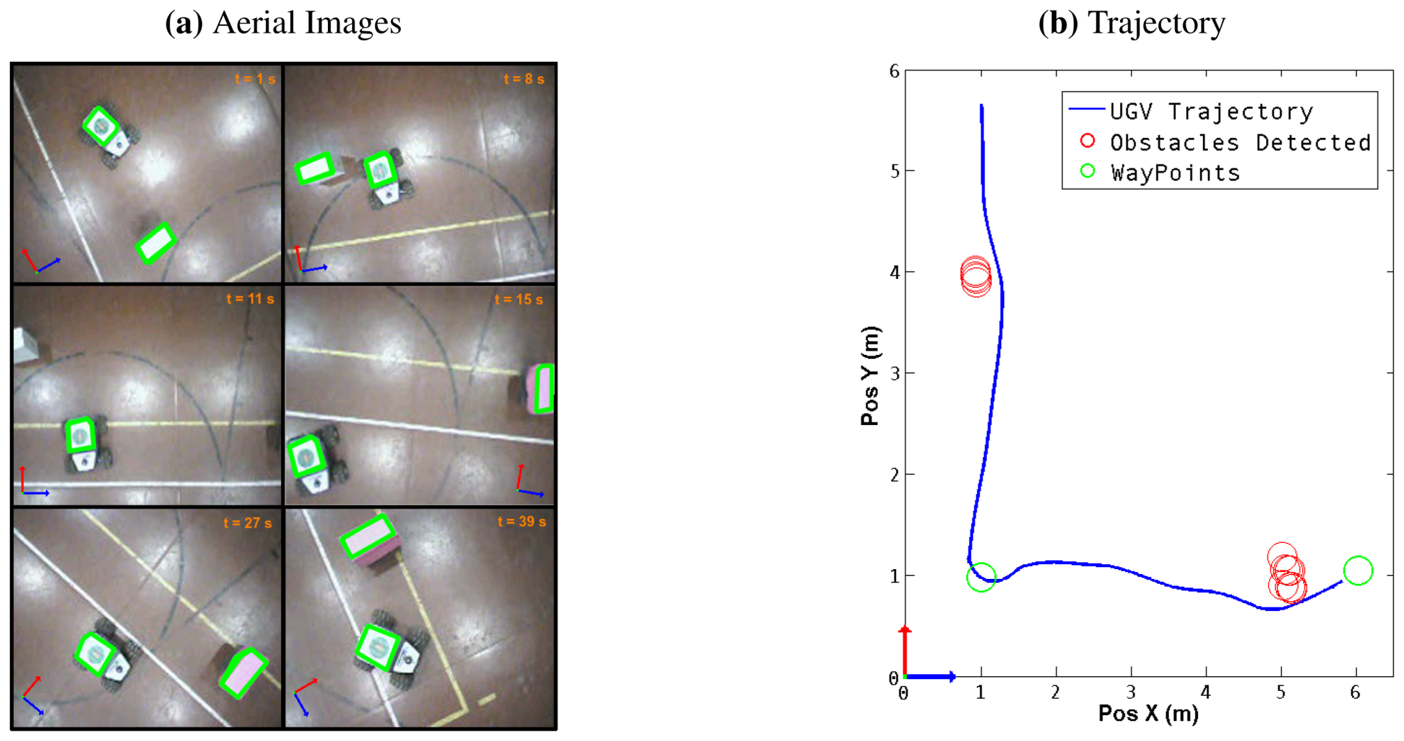
Figure 13 shows a sequence of aerial images obtained during a trajectory, with the objects identified in each frame, it also shows the trajectory obtained from the odometry of the UGV The variables measured during the experiment are shown in
Table 4.
The obstacles were successfully detected and avoided using the proposed system; the mean position and standard deviation of the observations are shown in
Table 5. It should be emphasized that the error in the estimated position of the obstacles was less than 0.15
meters in the last experiment. Moreover, the UGV maintained a mean safe distance from the obstacles of 0.3 meters. Therefore, despite the obstacles' position error, the UGV is unlikely to collide due to the safe distance between the obstacles.
Acknowledgments
This work was supported by the Robotics and Cybernetics Group at Technical University of Madrid (Spain), and funded under the projects ROTOS: Multi-robot system for outdoor infrastructures protection, sponsored by Spanish Ministry of Education and Science (DPI2010-17998), and ROBOCITY 2030, sponsored by the Community of Madrid (S-0505/DPI/000235).
References
- Choset, H.; Lynch, K.; Hutchinson, S.; Kantor, G.; Burgard, W.; Kavraki, L.; Thrun, S. Principles of Robot Motion: Theory, Algorithms, and Implementations; MIT Press: Boston, MA, USA, 2005. [Google Scholar]
- Krotkov, E. Position Estimation and Autonomous Travel by Mobile Robots in Natural Terrain. Kent Forum Book. 1997. Available online: http://www.ri.cmu.edu/pub_files/pub3/krofkov_eric_1997_2/krotkov_eric_1997_2.pdf (accessed on 3 January 2013).
- Moseley, M.B.; Grocholsky, B.P.; Cheung, C.; Singh, S. Integrated long-range UAV/UGV collaborative target tracking. Proc. SPIE 2009, 7332. [Google Scholar] [CrossRef]
- Li, W.; Zhang, T.; Klihnlenz, K. A vision-guided autonomous quadrotor in an air-ground multi-robot system. Proceedings of 2011 IEEE International Conference on Robotics and Automation (ICRA), Shanghai, China, 9–13 May 2011; pp. 2980–2985.
- Chaimowicz, L.; Kumar, V. Aerial shepherds: Coordination among uavs and swarms of robots. In Distributed Autonomous Robotic Systems 6; Springer: Tokyo, Japan, 2007; pp. 243–252. [Google Scholar]
- Ishikawa, S.; Kuwamoto, H.; Ozawa, S. Visual navigation of an autonomous vehicle using white line recognition. IEEE Trans. Patt. Anal. Mach. Intell. 1988, 10, 743–749. [Google Scholar]
- Matsumoto, Y.; Inaba, M.; Inoue, H. Visual navigation using view-sequenced route representation. Proceedings of 1996 IEEE International Conference on Robotics and Automation, Minneapolis, MN, USA, 22–28 April 1996; pp. 83–88.
- Dao, N.X.; You, B.J.; Oh, S.R. Visual navigation for indoor mobile robots using a single camera. Proceedings of 2005 IEEE/RSJ International Conference on Intelligent Robots and Systems (IROS 2005), Edmonton, AB, Canada, 2–6 August 2005; pp. 1992–1997.
- Cherubini, A.; Chaumette, F. Visual navigation with obstacle avoidance. Proceedings of 2011 IEEE/RSJ International Conference on Intelligent Robots and Systems (IROS), San Francisco, CA, USA, 25–30 September 2011; pp. 1593–1598.
- Grocholsky, B.; Dille, M.; Nuske, S. Efficient target geolocation by highly uncertain small air vehicles. Proceedings of 2011 IEEE/RSJ International Conference on Intelligent Robots and Systems (IROS), San Francisco, CA, USA, 25–30 September 2011; pp. 4947–4952.
- Dille, M.; Grocholsky, B.; Nuske, S. Persistent Visual Tracking and Accurate Geo-Location of Moving Ground Targets by Small Air Vehicles. Proceedings of AIAA Infotech@Aerospace Conference, St. Louis, MO, USA, 29–31 March 2011.
- Rao, R.; Kumar, V.; Taylor, C. Visual servoing of a UGV from a UAV using differential flatness. Proceedings of IEEE/RSJ International Conference on Intelligent Robots and Systems (IROS 2003), Las Vegas, NV, USA, 27 October–1 November 2003; pp. 743–748.
- Elfes, A.; Bergerman, M.; Carvalho, J.R.H.; de Paiva, E.C.; Ramos, J.J.G.; Bueno, S.S. Air-ground robotic ensembles for cooperative applications: Concepts and preliminary results. Proceedings of 2nd International Conference on Field and Service Robotics, Pittsburgh, PA, USA, 29–31 August 1999; pp. 75–80.
- Vidal, R.; Rashid, S.; Sharp, C.; Shakernia, O.; Kim, J.; Sastry, S. Pursuit-evasion games with unmanned ground and aerial vehicles. Proceedings of IEEE International Conference on Robotics and Automation, Seoul, Korea, 21–26 May 2001; pp. 2948–2955.
- Phan, C.; Liu, H. A cooperative UAV/UGV platform for wildfire detection and fighting. Proceedings of Asia Simulation Conference: 7th International Conference on System Simulation and Scientific Computing, Beijing, China, 10–12 October 2008; pp. 494–498.
- Chaimowicz, L.; Grocholsky, B.; Keller, J.F.; Kumar, V.; Taylor, C.J. Experiments in Multirobot Air-Ground Coordination. Proceedings of the 2004 International Conference on Robotics and Automation, Barcelona, Spain, 18–22 April 2004; pp. 4053–4058.
- MacArthur, E.Z.; MacArthur, D.; Crane, C. Use of cooperative unmanned air and ground vehicles for detection and disposal of mines. Proc. SPIE 2005, 5999, 94–101. [Google Scholar]
- Valente, J.; Barrientos, A.; Martinez, A.; Fiederling, C. Field tests with an aerial–ground convoy system for collaborative tasks. Proceedings of 8th Workshop de RoboCity2030-II: Robots Exteriores, Madrid, Spain, 2 December 2010; pp. 233–248.
- Snyder, J.P. Map Projections: A Working Manual; Supersedes USGS Bulletin 1532; U.S. Geological Survey, U.S. Government Printing Office: Washington, DC, USA, 1987. [Google Scholar]
- Gadeyne, K.; BFL: Bayesian Filtering Library. 2001. Available online: http://www.orocos.org/bfl (accessed on 3 January 2012).
- Garzón, M.; Valente, J.; Zapata, D.; Chil, R.; Barrientos, A. Towards a ground navigation system based in visual feedback provided by a mini UAV. Proceedings of the IEEE Intelligent Vehicles Symposium Workshops, Alcal de Henares, Spain, 3–7 June 2012.
- Reynolds, C.W. Steering Behaviors For Autonomous Characters. Proceedings of Game Developers Conference, San Jose, CA, USA, 15–19 March 1999; pp. 763–782.
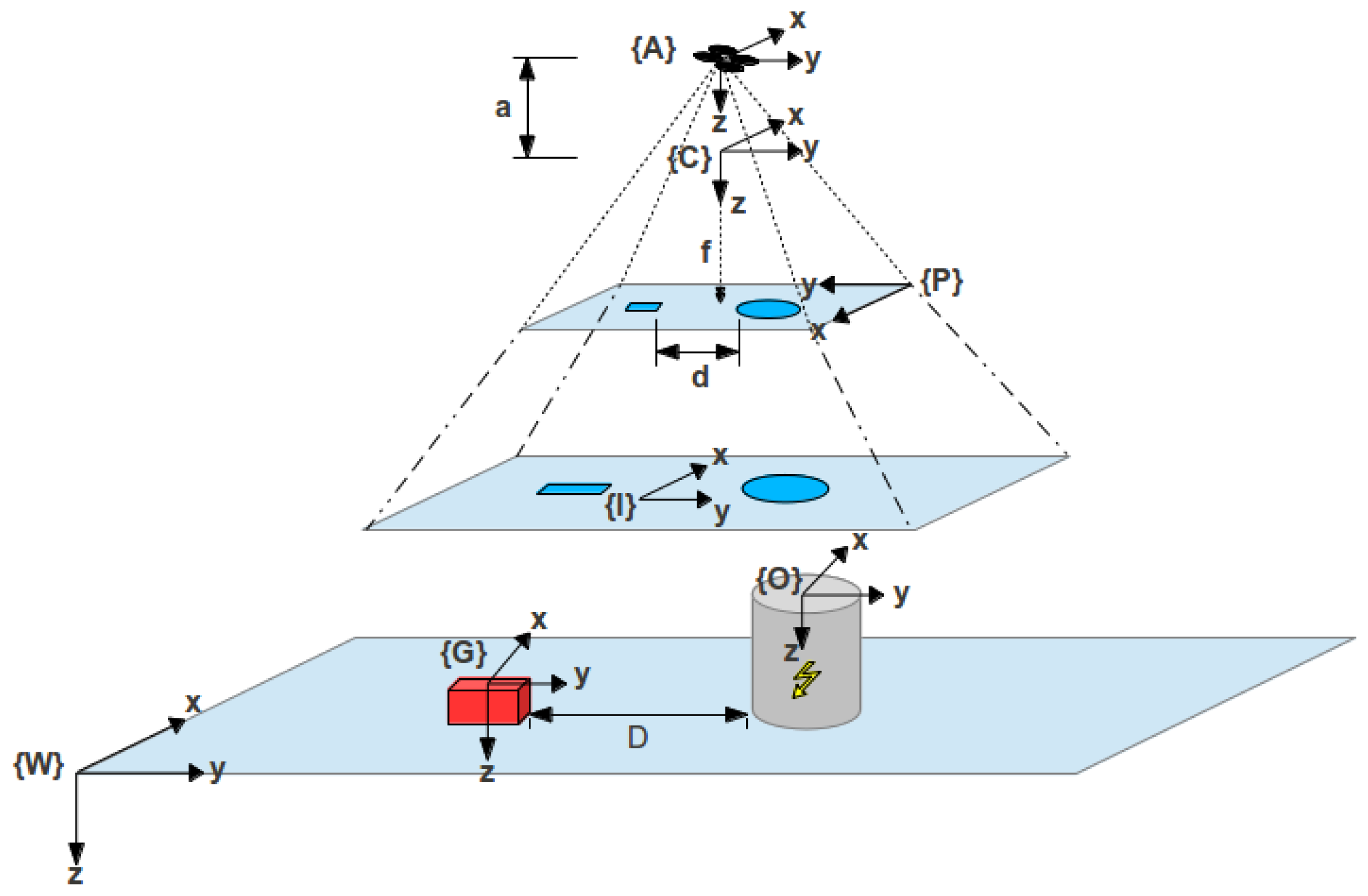
Figure 1.
Coordinate frames.
Figure 1.
Coordinate frames.
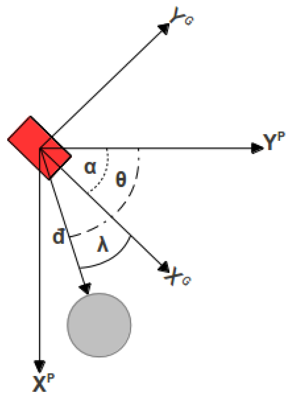
Figure 2.
UGV heading geometry. The angle of interest is given by γ = θ − α.
Figure 2.
UGV heading geometry. The angle of interest is given by γ = θ − α.
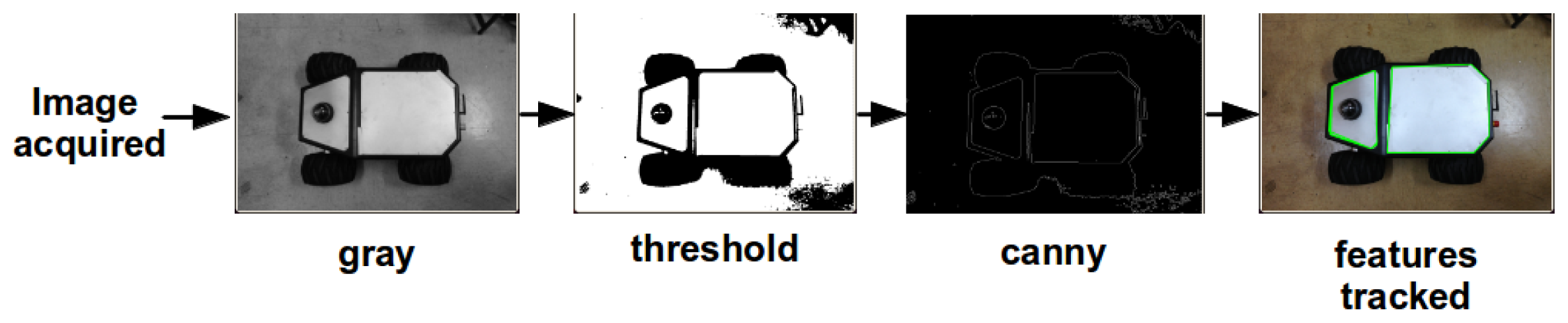
Figure 3.
Features extraction procedure example for a ground robot.
Figure 3.
Features extraction procedure example for a ground robot.
Figure 4.
Test Trajectory for EKF. A trajectory was performed in order to test the performance of the Extended Kalman Filter.
Figure 4.
Test Trajectory for EKF. A trajectory was performed in order to test the performance of the Extended Kalman Filter.
Figure 5.
Steering Behaviors. Two Behaviors (Seek and Avoid) and their corresponding vectors are shown.
Figure 5.
Steering Behaviors. Two Behaviors (Seek and Avoid) and their corresponding vectors are shown.
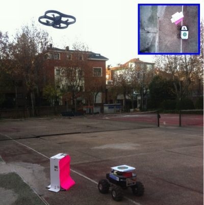
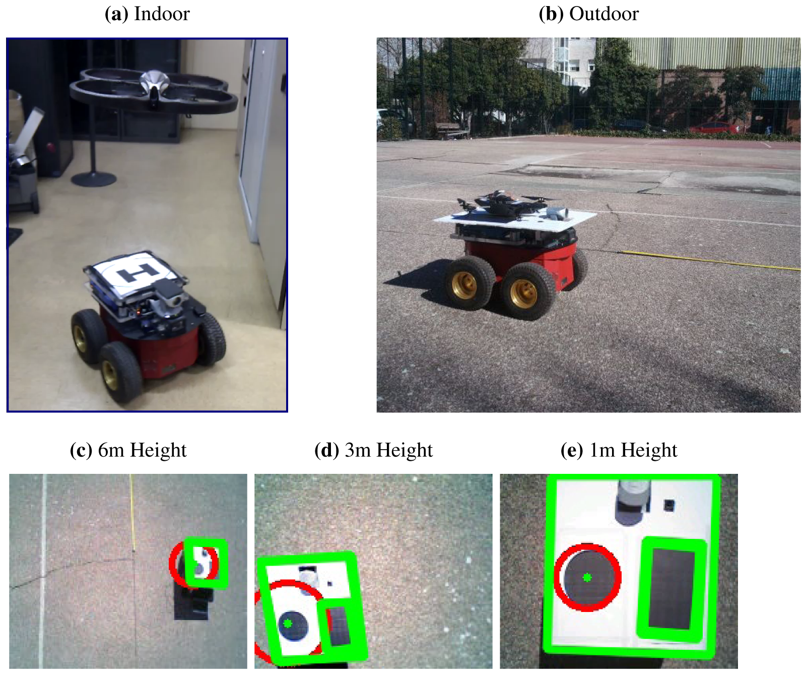
Figure 6.
UAV and UGV in the proposed environments (a) Simulated environment. (b) Real environment. The blue squares in each figure represent the image acquired from the camera on board the aerial robot.
Figure 6.
UAV and UGV in the proposed environments (a) Simulated environment. (b) Real environment. The blue squares in each figure represent the image acquired from the camera on board the aerial robot.
Figure 7.
Single obstacle Avoidance. The trajectory of the UGV while performing the avoidance maneuver, and the detected obstacle positions are shown.
Figure 7.
Single obstacle Avoidance. The trajectory of the UGV while performing the avoidance maneuver, and the detected obstacle positions are shown.
Figure 8.
Obstacle Position Estimation. The green line denotes the UGV position. The blue arrows determine the transformation from each robot position to the center of the obstacle marked with red circles.
Figure 8.
Obstacle Position Estimation. The green line denotes the UGV position. The blue arrows determine the transformation from each robot position to the center of the obstacle marked with red circles.
Figure 9.
Obstacle Position (Real vs. Estimated). The red circles denote the estimated obstacle position. The green one shows the real position of the obstacle and the blue is the mean value of the calculated positions. All positions were translated to a common reference frame.
Figure 9.
Obstacle Position (Real vs. Estimated). The red circles denote the estimated obstacle position. The green one shows the real position of the obstacle and the blue is the mean value of the calculated positions. All positions were translated to a common reference frame.
Figure 10.
Velocity Commands. The red line describes the UGV trajectory, and the blue arrows represent the velocity commands at each position.
Figure 10.
Velocity Commands. The red line describes the UGV trajectory, and the blue arrows represent the velocity commands at each position.
Figure 11.
Second Test Trajectory. The blue line describes the UGV trajectory. The red circles represent the obstacles found in the pathway and the green circles are the way-points.
Figure 11.
Second Test Trajectory. The blue line describes the UGV trajectory. The red circles represent the obstacles found in the pathway and the green circles are the way-points.
Figure 12.
Initial Tests with real robots: (a,b) Communication and hovering. (c), (d) and (e) Aerial Images captured at different heights.
Figure 12.
Initial Tests with real robots: (a,b) Communication and hovering. (c), (d) and (e) Aerial Images captured at different heights.
Figure 13.
Field tests: (a) Sequence of images obtained from the UAV while performing an obstacle-avoidance maneuver. The orientation is represented with a blue and red arrow for the X and Y axes. (b) The UGV trajectory read from the EKF is shown in blue, additional marks for the target and the obstacle have been added.
Table 1.
Mean Square Error and Standard Deviation of the calculated obstacle position.
Table 1.
Mean Square Error and Standard Deviation of the calculated obstacle position.
| Mean Square Error (m) | Standard Deviation |
|---|
| X Axis | 0.1954 | 0.4236 |
| Y Axis | 0.3333 | 0.3053 |
Table 2.
Mean Value and Standard Deviation for all the obstacles found in the Test Trajectory.
Table 2.
Mean Value and Standard Deviation for all the obstacles found in the Test Trajectory.
| Mean Pos X (m) | Std. Dev. X | Mean Pos Y (m) | Std. Dev. Y |
|---|
| Obstacle 1 | 441637.8 | 0.4743 | 4476756.3 | 0.6360 |
| Obstacle 2 | 441623.3 | 0.7489 | 4476768.4 | 0.5152 |
| Obstacle 3 | 441629.4 | 0.4939 | 4476761.9 | 0.2612 |
| Obstacle 4 | 441613.1 | 0.5246 | 4476755.1 | 0.4076 |
| Obstacle 5 | 441619.3 | 0.4924 | 4476749.7 | 0.3820 |
Table 3.
Frequencies and Time Consumption for image and data streaming and processing.
Table 3.
Frequencies and Time Consumption for image and data streaming and processing.
| Average Frequency (Hz) | Max. Period (s) | Min. Period (s) |
|---|
| Image Streaming | 10 | 0.446 | 0.003 |
| UAV Telemetry | 13 | 0.404 | 0.001 |
| UGV Telemetry | 20 | 0.051 | 0.049 |
| UGV Navigation System | 10 | 0.103 | 0.096 |
| Image and Data Processing | 37 | 0.102 | 0.010 |
Table 4.
Trajectory Parameters and Additional Information.
Table 4.
Trajectory Parameters and Additional Information.
| Trajectory Time: | 39 s |
| UGV Max Speed | 0.3 m/s |
| UGV Mean Speed | 0.2048 m/s |
| UAV Max altitude | 4.812 m |
| UAV Mean altitude | 4.51 m |
| Total Trajectory Distance: | 10.1999 m |
Table 5.
Mean Value and Standard Deviation for the obstacles found in the trajectory.
Table 5.
Mean Value and Standard Deviation for the obstacles found in the trajectory.
| Mean Pos X (m) | Std. Dev. X | Mean Pos Y (m) | Std. Dev. Y |
|---|
| Obstacle 1 | 0.9896 | 0.0194 | 4.1373 | 0.0468 |
| Obstacle 2 | 5.0930 | 0.1143 | 1.1158 | 0.0492 |
© 2013 by the authors; licensee MDPI, Basel, Switzerland. This article is an open access article distributed under the terms and conditions of the Creative Commons Attribution license (http://creativecommons.org/licenses/by/3.0/).


