Magnetic Field Analysis of Lorentz Motors Using a Novel Segmented Magnetic Equivalent Circuit Method

Abstract
: A simple and accurate method based on the magnetic equivalent circuit (MEC) model is proposed in this paper to predict magnetic flux density (MFD) distribution of the air-gap in a Lorentz motor (LM). In conventional MEC methods, the permanent magnet (PM) is treated as one common source and all branches of MEC are coupled together to become a MEC network. In our proposed method, every PM flux source is divided into three sub-sections (the outer, the middle and the inner). Thus, the MEC of LM is divided correspondingly into three independent sub-loops. As the size of the middle sub-MEC is small enough, it can be treated as an ideal MEC and solved accurately. Combining with decoupled analysis of outer and inner MECs, MFD distribution in the air-gap can be approximated by a quadratic curve, and the complex calculation of reluctances in MECs can be avoided. The segmented magnetic equivalent circuit (SMEC) method is used to analyze a LM, and its effectiveness is demonstrated by comparison with FEA, conventional MEC and experimental results.1. Introduction
In recent years, the Lorentz motor (LM) has been applied widely as an actuator to generate forces with direct drive, fast response time, great precision, low noise, low vibration, etc. [1,2]. Despite the above superior performance, some properties like the power-to-weight ratio, efficiency, speed range and cost etc., remain to be improved [3,4]. It has been shown in the literature that flux leakage and magnet end flux have substantial effects on the magnetic analysis [5–8], so that an accurate magnetic flux density (MFD) distribution model of the LM, especially including flux leakage and magnet end flux, is critical.
Different methods, including analytical methods, numerical methods, and magnetic equivalent circuit (MEC) methods, have been employed to model MFD distribution [9]. Analytical methods, based on the Maxwell equations, are a powerful tool, but they can hardly model the slot effect and flux leakage [3,4]. Among numerical methods, FEA is used extensively in the design of motors, however it does not specify the functional form of the relationship between the MFD and geometrical parameters of the motor [10]. Furthermore, the computational cost is enormous.
MEC, based on the Kirchhoff's law, has become an efficient magnetic analysis method [3,9]. Advantages such as moderate accuracy, reduced model complexity and low computational cost, make it an effective means in the design of motors [9,11,12].
MEC was originally proposed and developed in [13–16]. A synchronous machine model was presented in [17–20]. In [21] and [22], mesh-based MECs were discussed. In [5–7,23], flux leakage was modeled by different means, which is crucial in the analysis of motors. Techniques to incorporate MECs with finite-element models were proposed in [24–27]. An accurate yet simple method for predicting the flux density distribution and iron losses in linear PMSM was presented in [28]. In [8], leakage flux associated with a brushless permanent magnet motor utilizing a segmented stator core was analyzed.
However, MEC models always treat the permanent magnet (PM) as one common source and all branches of MEC are coupled together to become a large MEC network. If flux leakage and magnetic end are also considered, the complexity of these models has to be increased and the analysis process would become extremely complicated as well.
This paper presents a segmented magnetic equivalent circuit (SMEC) method, which can be used to analyze the magnetic field of the LM with considerably reduced complexity. The quadratic MFD distribution curves based on the sub-MECs are also proposed to analyze air-gap MFD distribution and to predict the relationship between the air-gap MFD and parameters of the LM. This SMEC method and the curve prediction method are validated by comparison with FEA, conventional MEC method and experimental results.
2. Structure of the Lorentz Motor
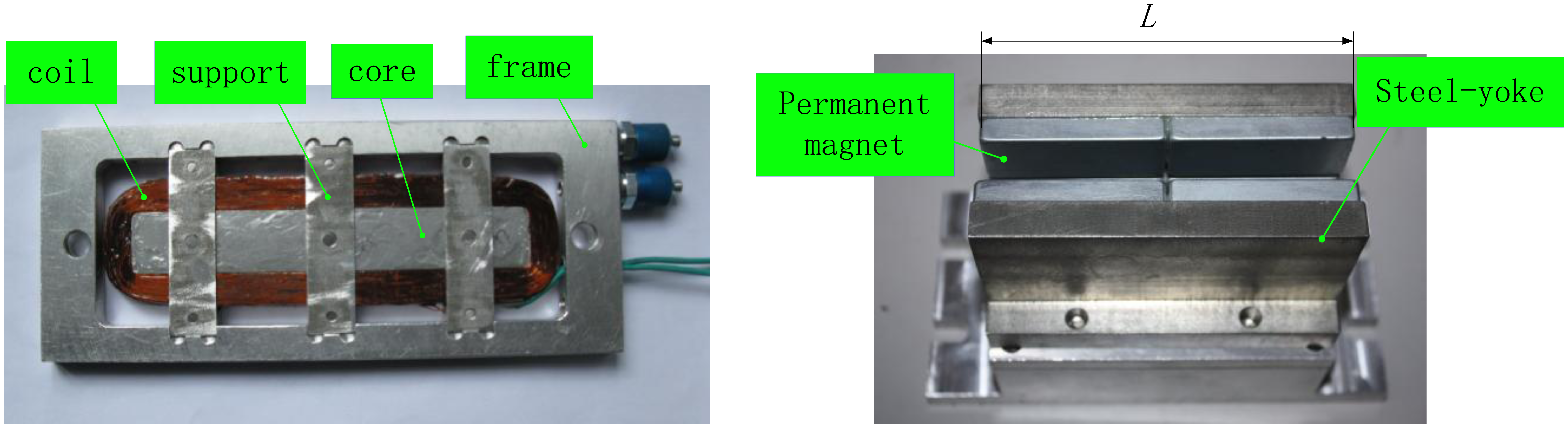
A LM is used as the actuator of an isolator since the Lorentz force can be characterized “fast”. Figure 1 shows the structural configuration of the LM. The LM is mainly composed of a mover, a stator and some auxiliaries. The coil is installed in a frame which is sealed by covers.
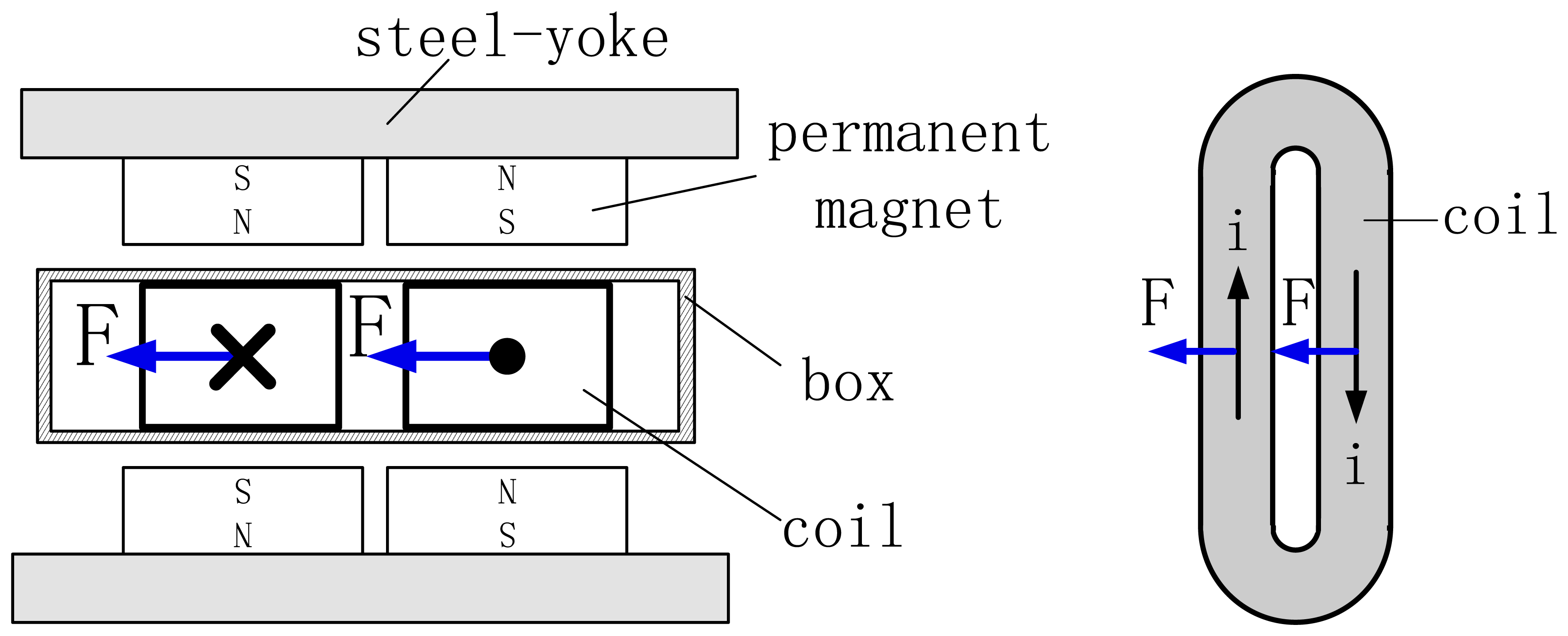
The working principle of a Lorentz motor is that a Lorentz force will be exerted on the coil when an electric current flows across it. Electric current I and MFD B are perpendicular to each other, and the direction of the Lorentz force F will be decided by Fleming's left-hand rule. The layout of the LM is illustrated in Figure 2. In order to make the Lorentz force uniform on both sides of the coil, the PMs are stuck on the steel-yoke with alternating polarities. The coil is laid in the air-gap between two opposite magnet poles.
3. SMEC Analysis
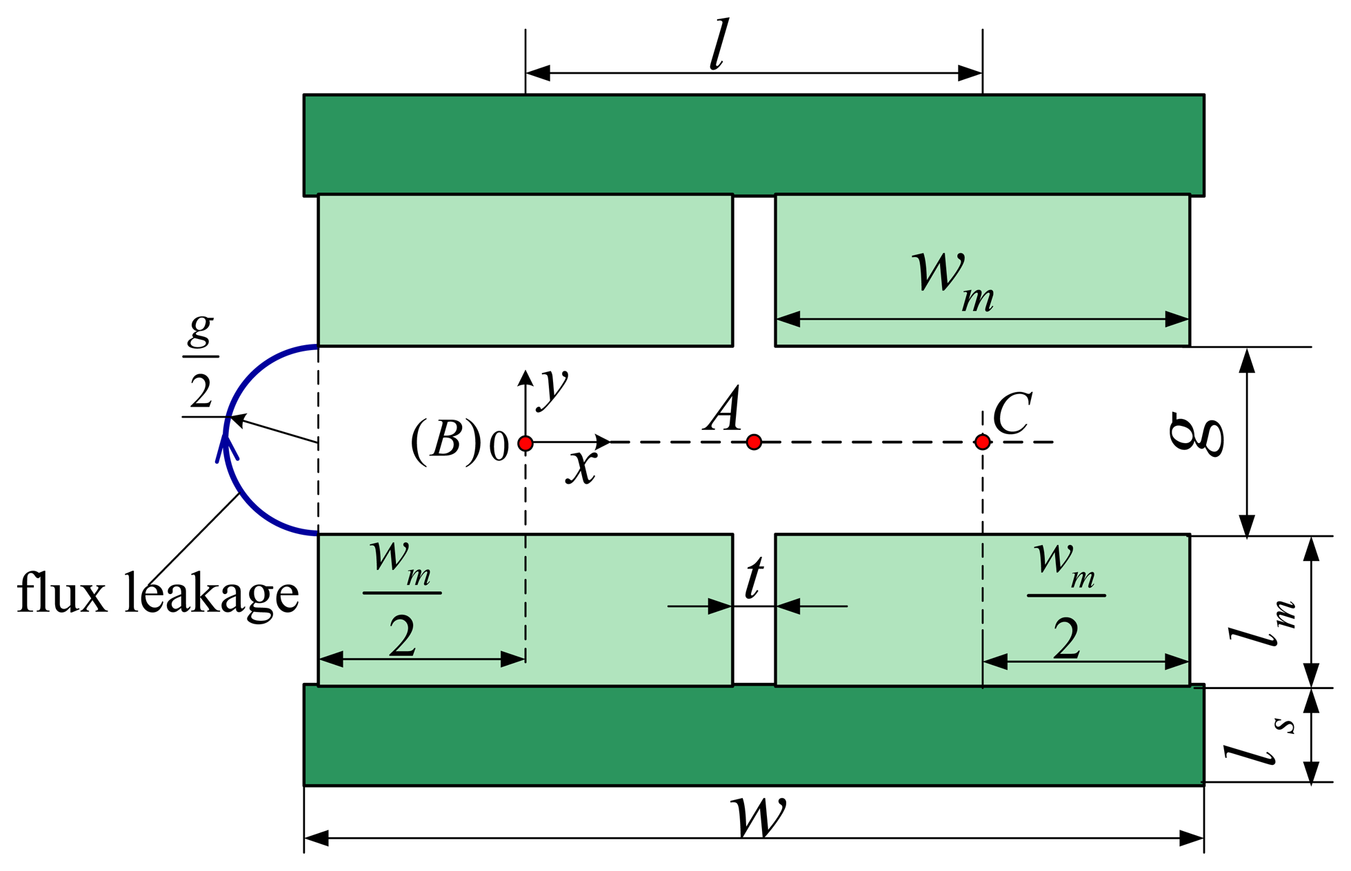
The structure of the stator is shown in Figure 3.
The air-gap between the two magnet poles has width g; t is the gap distance between adjacent poles; lm and ls represent the thickness of the PM and steel-yoke, respectively. w and wm denote the width of the steel-yoke and PM, respectively.
3.1. Conventional MEC
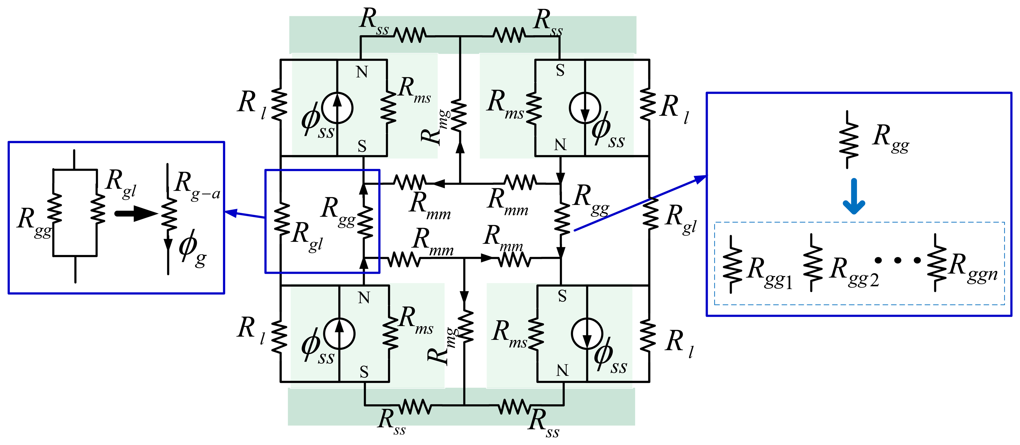
The conventional MEC model [4,17,19,29] of the LM is shown in Figure 4. In Figure 4, ϕss is the flux source of the magnet pole; Rms stands for the reluctance corresponding to the flux ϕss. Rgg represents the air-gap reluctance. Rss denotes the reluctance in the steel-yoke. Rgl and Rl are the different leakage reluctances. Rmg denotes the reluctance due to magnet pole-to-pole leakage, and Rmm represents the reluctance of the leakage flux between adjacent poles.
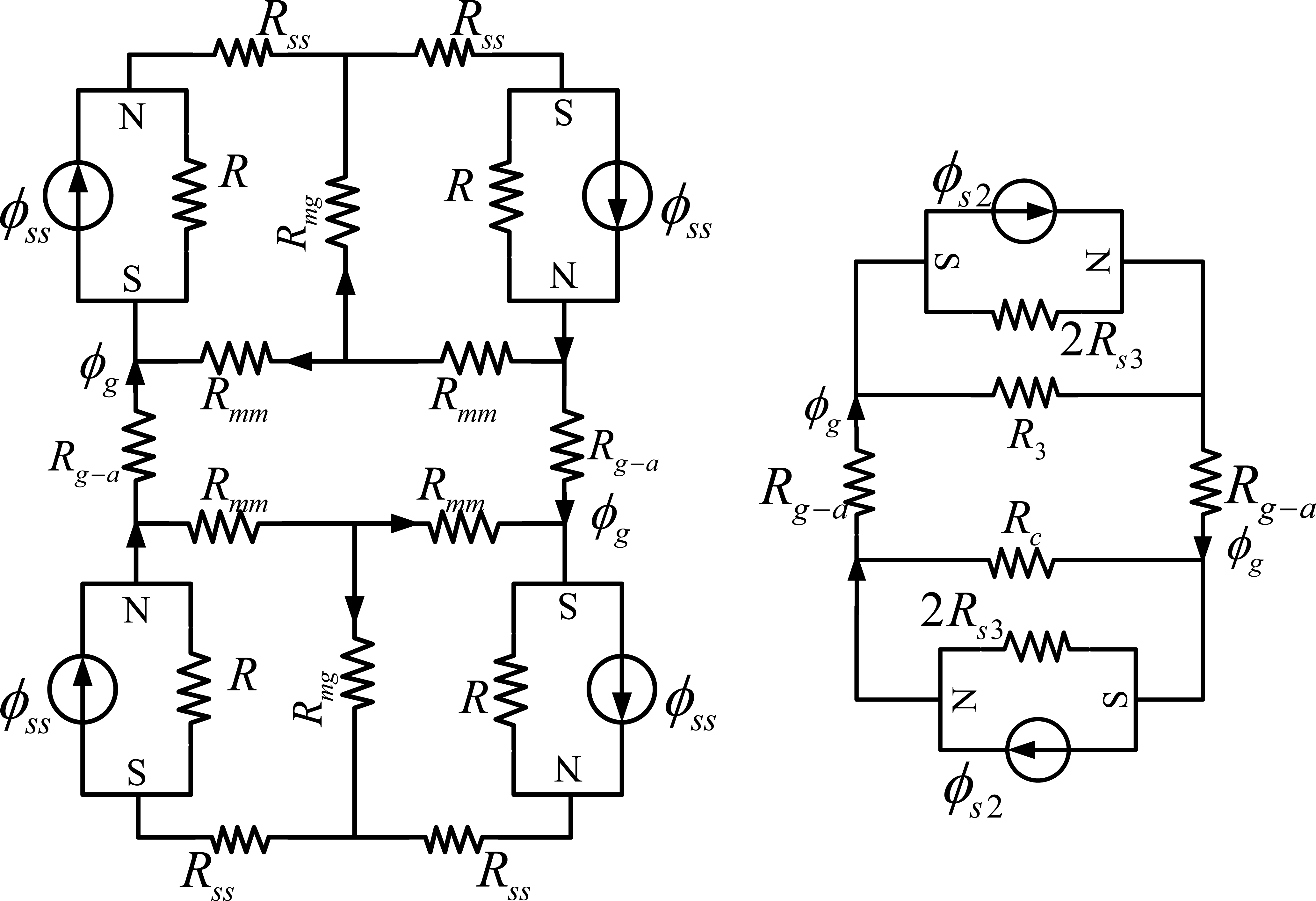
Using the equivalent-resistance theory, the MEC in Figure 4 can be simplified as in Figure 5. The value of these reluctances can be calculated by applying Ampere's law as:
The reluctance Rmm can be calculated as follows [28]:
The flux leakage tube of Rgl and Rl is a half cylinder and can be expressed as [1,12,29]:
From Figures 4 and 5 and by flux division, the analytical expressions for reluctance Rgg and Rgl can be obtained as:
If the magnetic flux is divided by the corresponding area that the magnetic flux through, the MFD B can be obtained. In the conventional lump-parameter MEC model, the reluctance is modeled by a single constant (e.g., Rgg), thus the spatial variation of MFD cannot be resolved.
In order to model the reluctance more accurately, the air-gap reluctance has to be divided into Rggi (I = 1, 2…n) as shown in Figure 4. Similarly, Rl, Rmg and Rmm should also be divided into Rli, Rmgi and Rmmi (I = 1, 2…n), respectively, resulting in a very large MEC. Since all the circuits are interleaved, the whole MEC has to be solved to obtain any local values. Furthermore, the effect of a local change in the LM will spread over the whole MEC, and the whole MEC has to be solved again to obtain changes on every local values.
3.2. MEC Segmentation
In a magnetic field, magnetic flux lines (MFLs) make a closed route from the north to the south and don't cross each other. Similarly, if the MFLs are separated into groups, no group crosses another. In LM, the leakage flux appears at the edge of permanent magnets. If the MEC of the LM can be divided into three sub-MECs and every sub-MEC has independent flux sources and loop, the leakage flux only appears in the lateral groups and the middle MEC is ideal. If the analysis is based on an ideal sub-MEC from all sub-MECs, it will be simple and accurate. For every independent sub-MEC, if parameter of the LM changes in the design, it only affects the corresponding sub-MEC.
In the design and optimization of motors, it is necessary yet difficult to predict accurately MFD distribution of the air-gap. In order to overcome this problem, quadratic MFD distribution curves based on the analysis of the SMEC are used to obtain the MFD distribution curve of the air-gap. The analysis also holds for nonlinear materials, because the magnetic saturation can be negligible for a LM with larger air gap. Additionally, to avoid magnetic saturation, the geometric size and material properties of the steel-yoke have been chosen elaborately (such that ls > lm as shown in Table 1). A 2-D structure of the LM stator and the SMECs are shown in Figures 3 and 6, respectively.
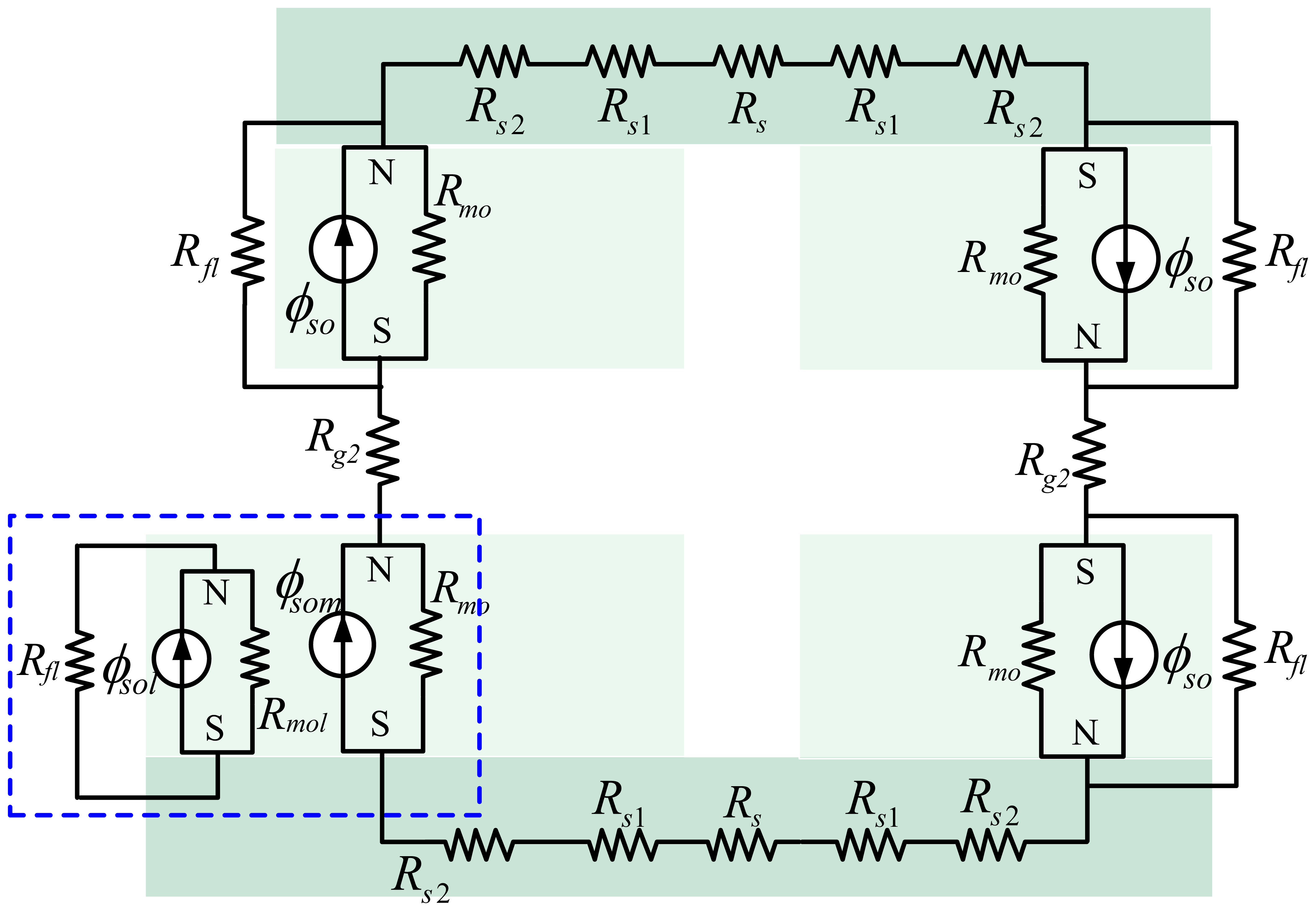
According to the SMEC method, the flux source is divided into three sub-parts (ϕsi, ϕsm, ϕso) and three sub-MECs (the inner MEC, the middle MEC and the outer MEC) are sketched in Figure 6.
In all sub-MECs, the middle MEC is the smallest. In its air-gap, MFLs are deemed even without leakage and spreading. The middle MEC is closest to being ideal and affected only slightly by flux leakage in fact. Additionally, the smaller is the middle MEC, the more ideal is this sub-MEC. If necessary, the outer MEC and the inner MEC can be divided further in the segmented decoupling method.
In Figure 6, ϕsi, ϕsm and ϕso are the flux sources of the magnet pole in the three sub-MECs, respectively; Rmi, Rm and Rmo stand for the reluctances corresponding to the fluxes ϕsi, ϕsm and ϕso respectively. Rg, Rgl and Rg2 represent the air-gap reluctances in the three sub-MECs. Rs, Rs1 and Rs2 denote the different reluctances in the steel-yoke. Rflis the leakage reluctance of the outer MEC and RML is the leakage reluctance of the inner MEC.
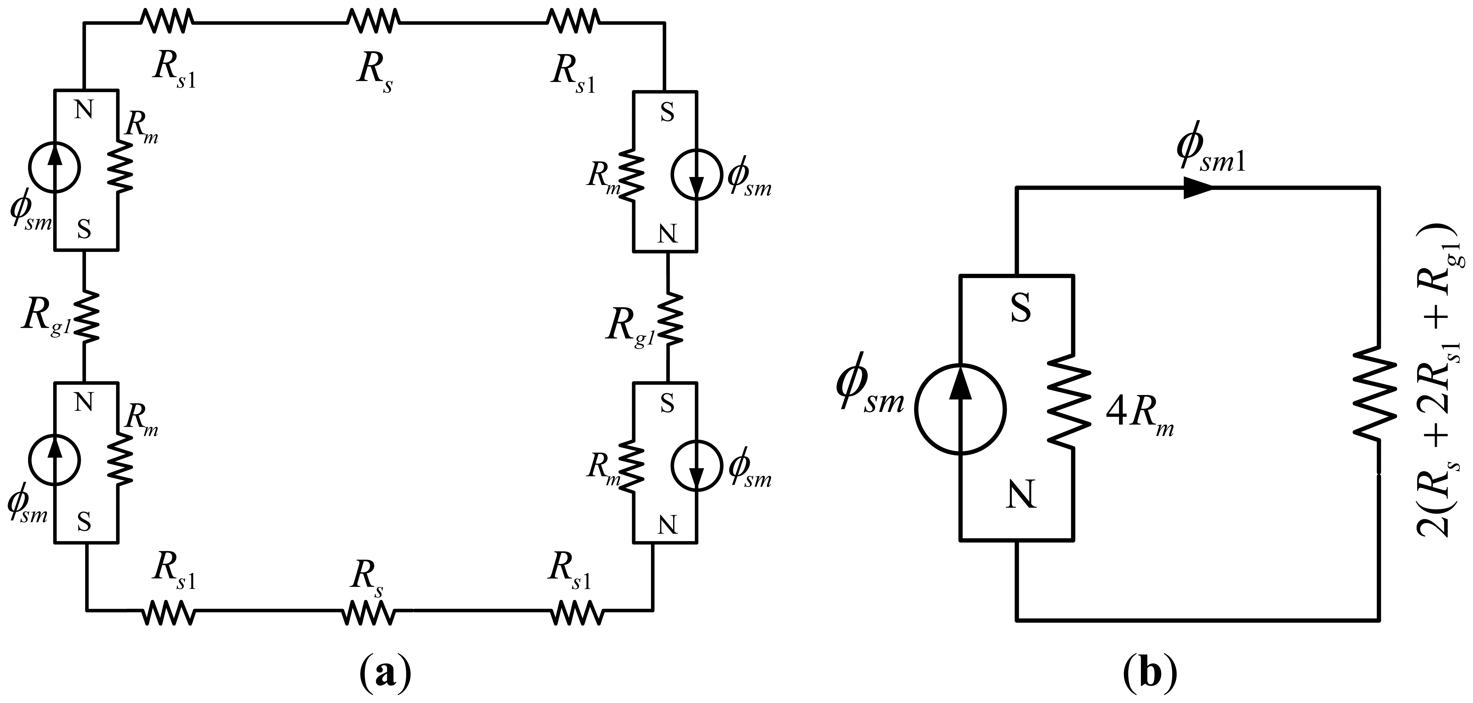
3.3. Analysis of the Middle MEC
Figure 7(a) depicts the middle MEC. It can be simplified as in Figure 7(b), using the equivalent-resistance theory. According to the width of the corresponding flux tubes of Rs, Rs1 and Rs2 as illustrated in Figure 6, applying the formula of resistance yields:
Here, L is the length of the PM in the LM as shown in Figure 1. Ag and Am represent the flux surface areas of the air-gap and PM in the middle MEC, respectively.
In the middle MEC, Rs + 2Rs1 can be expressed as:
By flux division:
Substituting Equation (9) into Equation (11) yields:
Here, ϕg1 is the air-gap flux that passes through Rg1. Bsm and Bg1 are MFDs corresponding to fluxes ϕsm and ϕg1, respectively. Asm is the flux surface area of the magnet pole. μ0 and μrm represent air permeability and the relative permeability of the PM, respectively. Hc denotes the magnetic coercive force.
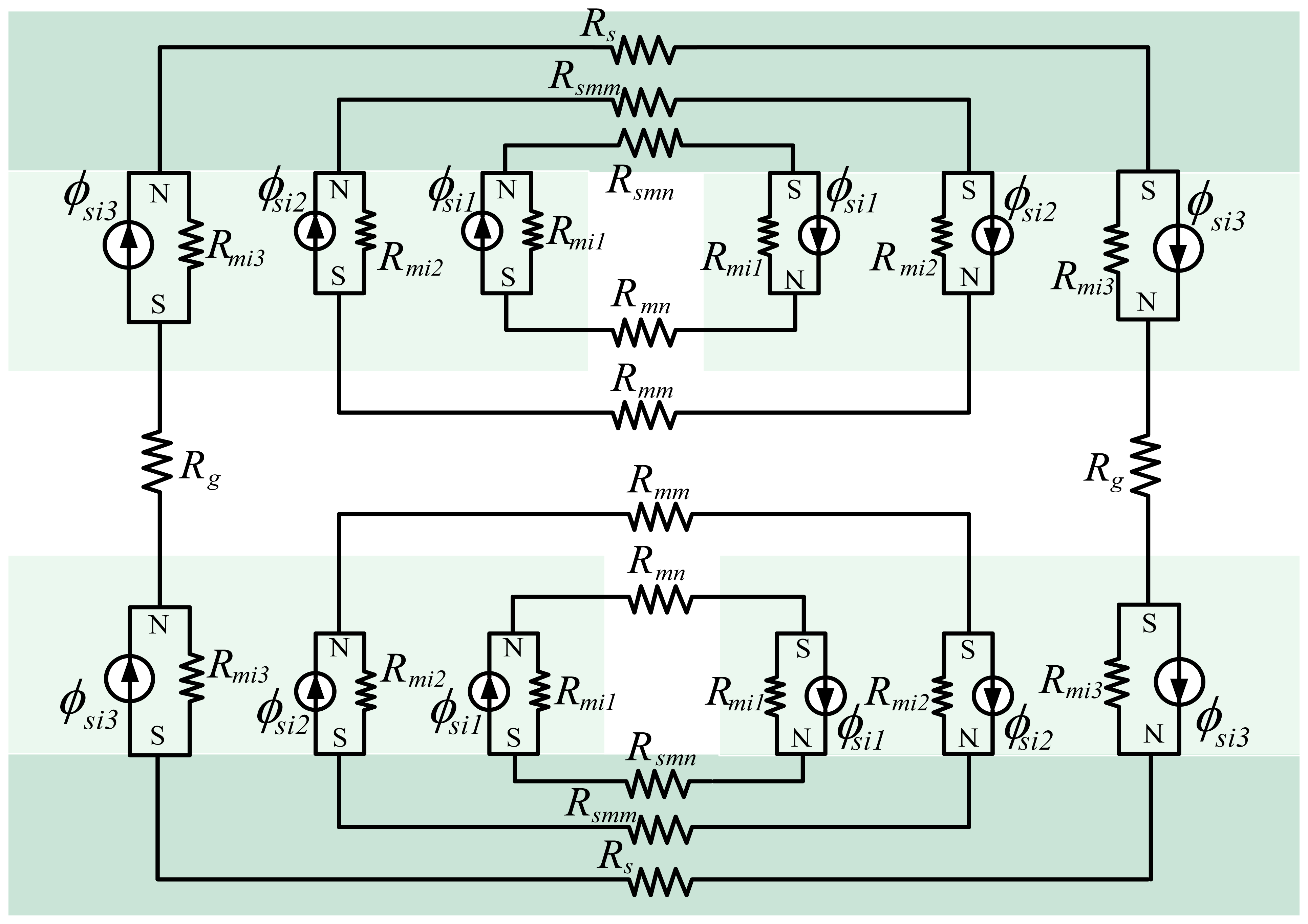
3.4. Analysis of the Inner MEC
The inner MEC can be divided further with the above method as illustrated in Figure 8. The inner MEC is composed of three sub-MECs as shown in Figure 8.
By definition, ϕsi1 and ϕsi2 are the flux-leakage sources of the magnet pole in gap t and air-gap g, respectively. ϕsi3 is the flux source of the magnet pole; Rmi1, Rmi2 and Rmi3 are the reluctances corresponding to fluxes ϕsi1, ϕsi2 and ϕsi3, respectively. Rmn and Rmm represent the different reluctances due to magnet pole-to-pole leakage. Rsmn, Rsmm and Rs denote the reluctances of the steel-yoke in different MECs.
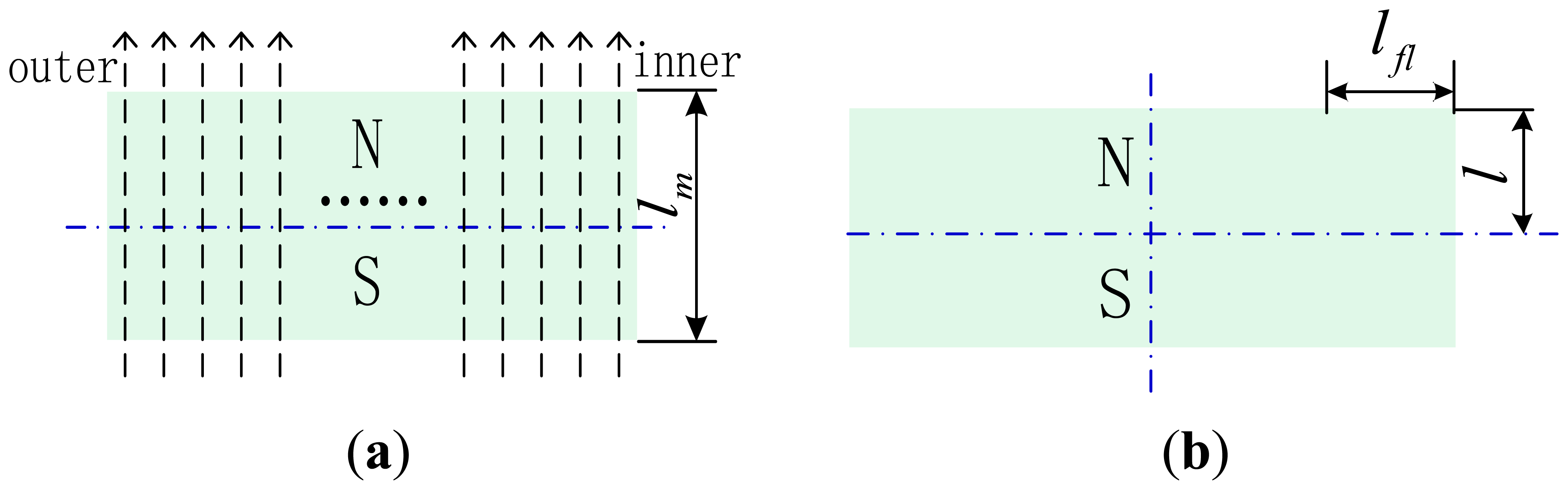
Here, it is assumed that under ideal conditions, MFLs pass through the PM evenly without leakage as illustrated in Figure 9(a). Then, magnet-end pole-to-pole leakage occurs. Here, lm is the thickness of the magnet pole and lfl is the width of the flux source of flux leakage as shown in Figure 9(b). Because flux leakage occurs mainly near the ends of the magnet pole, the width of the flux source of flux leakage lfl must be smaller than half of lm. In addition, for weak flux leakage, lfl is assumed to satisfy lm/4 = 1.875 mm.
A reference frame, x-o-y, is attached on the central point of the air-gap as illustrated in Figure 3. On the symmetry line of air-gap g, the MFD decreases gradually. It is further assumed that MFD By-in can be expressed as a function of x. For simplicity, it is also assumed that this function can be written as:
Here, x is the coordinate in the x-axis, By-in represents the MFD at location x of y-coordinate axe in Figure 3, and parameters a, b and c are constant. An analytical expression for the above analysis can be written as:
The route of the flux leakage can be regarded approximately as an ellipse as shown in Figure 10. Since the MFD of air-gap g is symmetrical about the x-axis, it can be deduced that the MFD of point-A ((wm+ t)/2, 0) is 0 as shown in Figure 3 and the analytical expression can be written as:
The MFD of the coordinate origin, as shown in Figure 3, can be calculated from:
3.5. Analysis of the Outer MEC
Similar to the inner MEC, the outer MEC can be divided further. Since the four sub-MECs are all similar, only one of them (in the dashed box) is divided further as in Figure 11.
Referring to the literatures [1,12,29], the flux leakage tube is a half cylinder as shown in Figure 3. MFD By-out can be expressed as a function of x:
Here, By-out represents the MFD at location x of y-coordinate axe in Figure 3, and parameters a1, b1 and c1 are constant.
On the boundary of the outer MEC, the MFD can be obtained by solving:
When flux leakage is weak, it can be ignored, or simplified as in the analysis of the inner MEC. Since the number of MFL is a constant, the following equation can be obtained:
By dividing every sub-MEC, the whole magnetic field of the LM can be divided into some separate and simple sub-MECs. In this way, every magnetic field of the LM can be analyzed independently and easily.
4. Validation of SMEC
2-D FEA has been carried out to validate the SMEC method. The main parameters of the LM are given in Table 1.
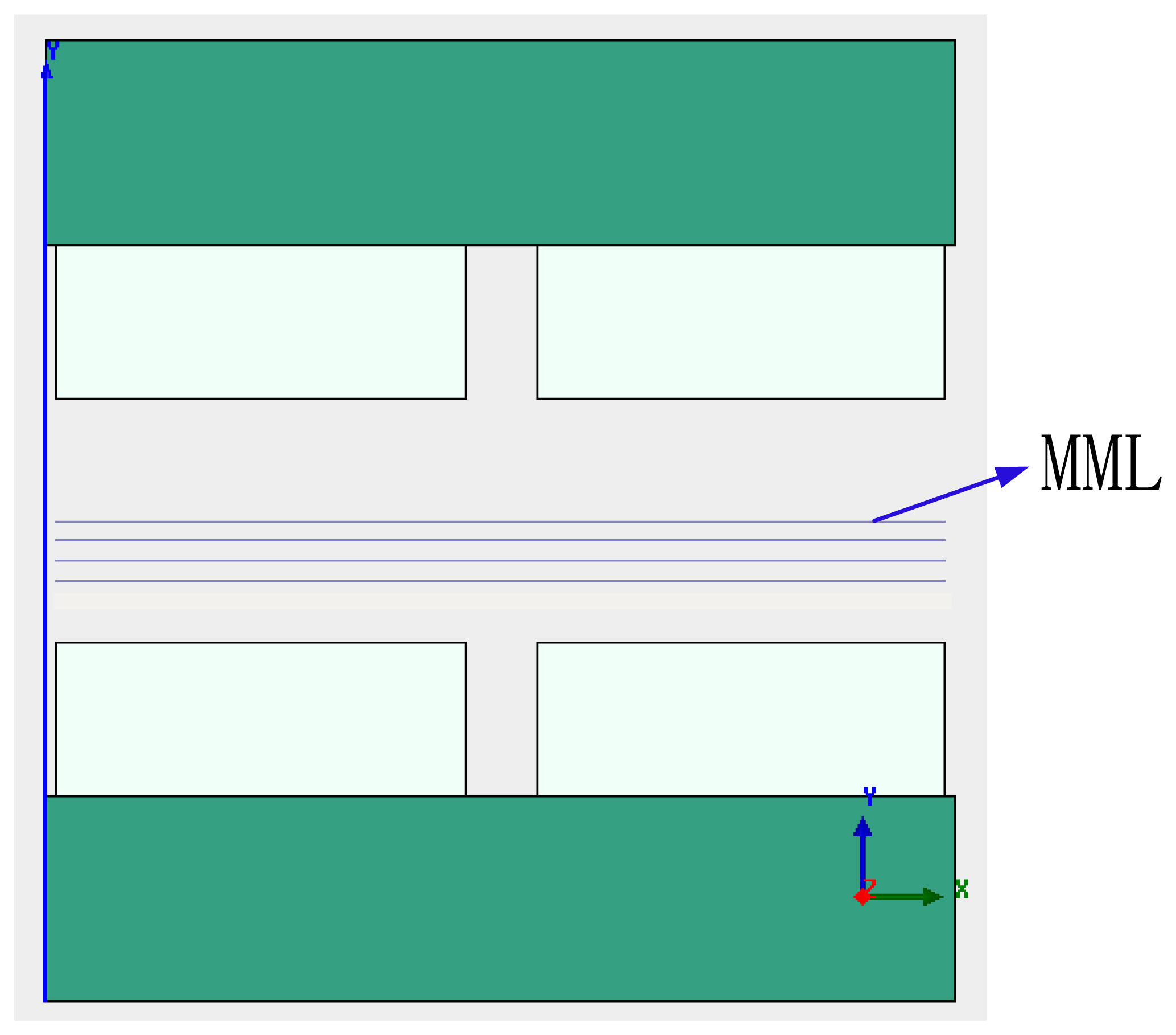
A group of lines that are parallel with the x axis and equally spaced with a distance 1 mm are drawn in air-gap g as shown in Figure 12. In the group of lines, the line of symmetry is called the magnetic middle line (MML) as illustrated in Figure 12.
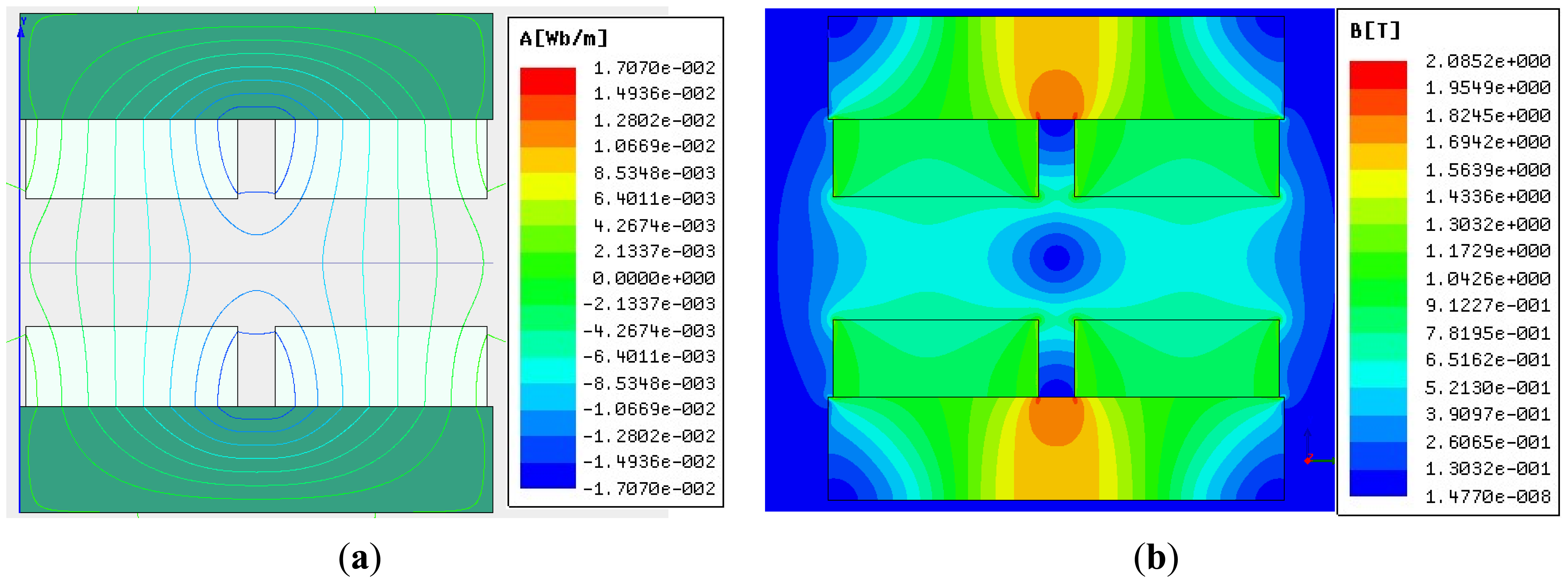
Figure 13 shows the flux contour profile and MFD distribution of the air-gap in the LM. Figure 13(b) shows the MFD of the air-gap in the LM. The MFD of point A (as shown in Figure 3) is 0. In the location of the middle sub-MEC, MFLs are nearly ideal.
Variation of the group of lines with coordinate x is plotted in Figure 14. The curves indicate that the MFD in the middle part of these lines changes less than 0.1 T. The Lorentz force is exerted on the coil placed in this part. Thus, it is critical to analyze the MFD in this middle part. From Figure 14, it can be seen that all the curves have the same qualitative trend.
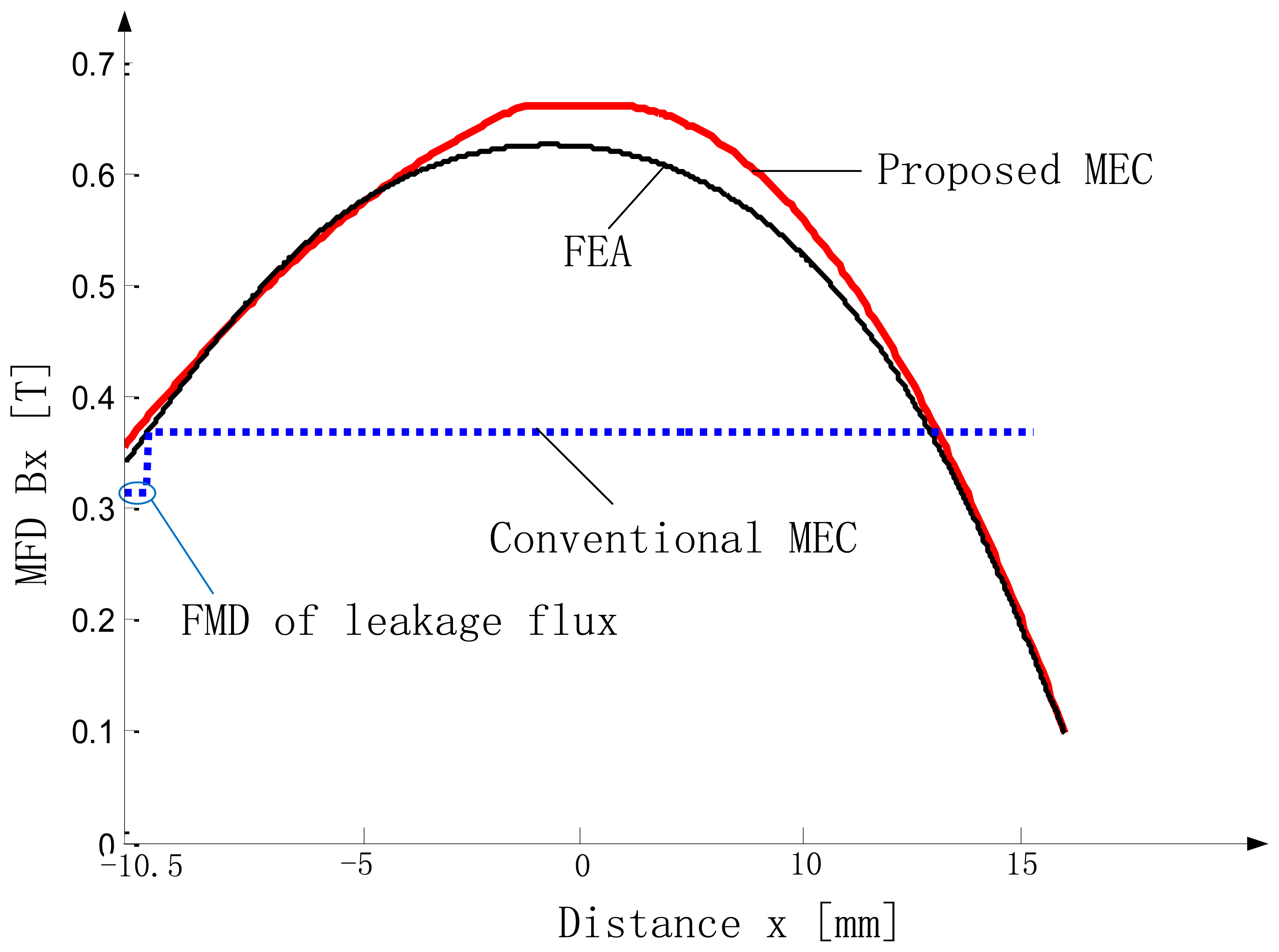
The MFD on MML is depicted in Figure 14. Since the curve is symmetric, it is enough to study half of it. In Figure 15, the curves, obtained from the proposed SMEC (Equations (5)–(7) and (9)–(11)), 2-D FEA and conventional MEC, are shown for comparison.
As illustrated in the figure, results of the proposed SMEC method are in very good agreement with 2-D FEA and the difference is less than 6%, while the difference between conventional MEC analysis and 2-D FEA is much larger.
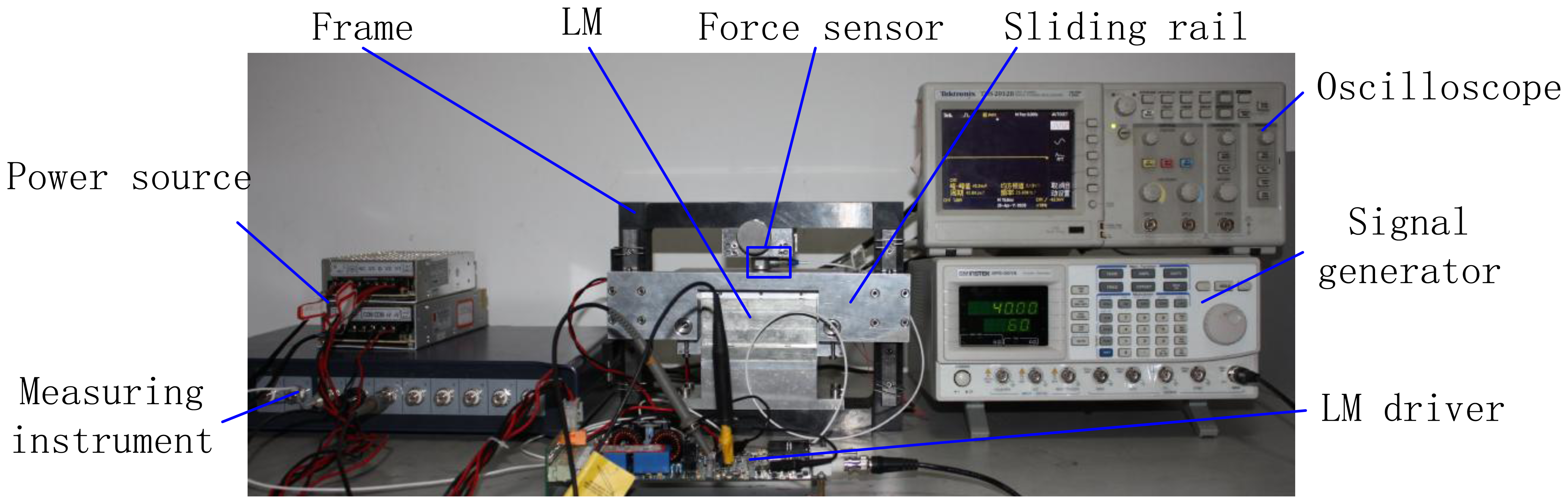
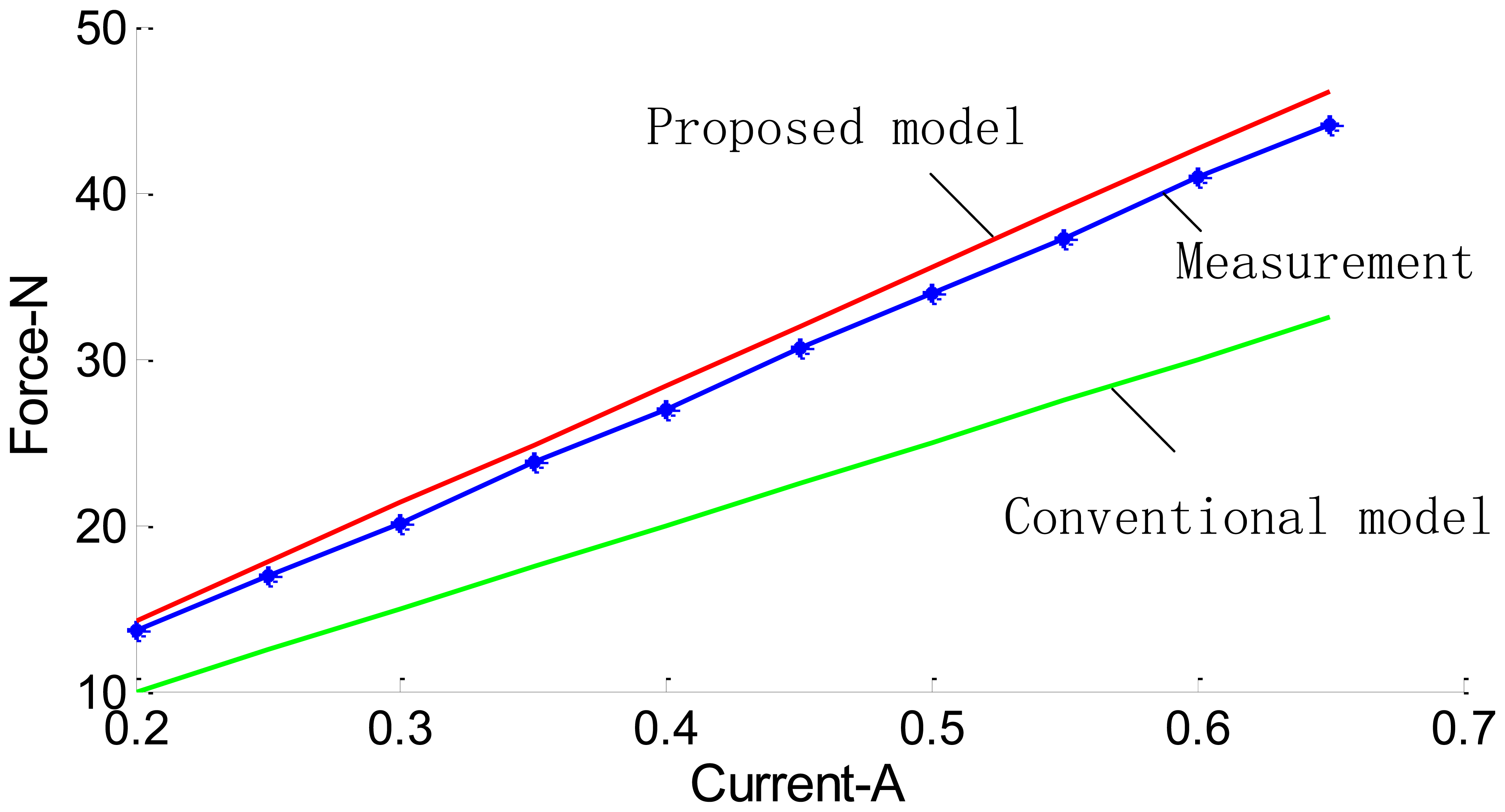
To obtain the relation between thrust force and current in the LM, the corresponding experiment is conducted as shown in Figure 16. After the air-gap MFD of the LM has been obtained, according to the Lorentz law, the thrust force of the LM is calculated using the integral method [1,30]. Figure 17 shows the thrust as a function of primary current density. It can be seen that the proposed SMEC method is more accurate than the existing method.
From Figures 15 and 17, it is evident that the spatial variation of the air-gap MFD can be obtained more accurately by the SMEC method than the conventional MEC method. Thus, the thrust of the LM can be predicted more accurately. This SMEC method can be very effective in the design and optimization of LMs.
In the proposed SMEC method (Figure 6), each sub-MEC can be solved independently, and any local change will affect only the local sub-MEC. In other words, using the SMEC method, modeling of the LM can be parallelized, and the computational gain increases significantly with the increase of the number of elements in the LM. At the same time, with our proposed SMEC method, spatial variation of MFD can be resolved accurately (Figure 15), which is another advantage over the conventional MEC method.
5. Conclusions
A simple yet accurate SMEC method for predicting air-gap MFD distribution of LMs is proposed, in which segmented sub-MECs are decoupled. The magnetic field of the LM can be analyzed with considerably reduced complexity and the relation between the air-gap MFD and the parameters of LM can be established easily. The size of middle sub-MEC is the smallest one, which approaches an ideal situation and can be solved accurately by MEC equations. In the middle part of the LM air-gap, the MFD is approximately uniform. Based on the study of the middle MEC, relationship between this part of the MFD and parameters of the LM can be obtained by analyzing the middle MEC. After analyzing sub-MECs, quadratic curves are used to predict the air-gap MFD of the LM. The calculation of complex reluctances of MECs is avoided. Prediction accuracy of the proposed method is verified by comparison with FEA results, and is less than 6%. The comparison between proposed SMEC and conventional MEC shows the advantage of the proposed SMEC. The proposed SMEC method can be used in LM design and optimization with improved simplicity and desirable accuracy.
Acknowledgments
The work was supported by the National Natural Science Foundation of China (No. 51121002, No. 51235005, No.51175196) and the Major State Basic Research Development Program of China (973 Program) (No. 2009CB724205).
References
- Chen, Y.D.; Fuh, C.C.; Tung, P.C. Application of voice coil motors in active dynamic vibration absorbers. IEEE Trans. Magn. 2005, 41, 1149–1154. [Google Scholar]
- Chou, P.C.; Lin, Y.C.; Cheng, S. Enhancement of optical adaptive sensing by using a dual-stage Seesaw-Swivel actuator with a tunable vibration absorber. Sensors 2011, 11, 4808–4829. [Google Scholar]
- Yilmaz, M.; Krein, P.T. Capabilities of Finite Element Analysis and Magnetic Equivalent Circuits for Electrical Machine Analysis and Design. Proceeding of IEEE Annual Power Electronics Specialists Conference, Rhodes, Greece, 15– 19 June 2008; pp. 4027–4033.
- Sheikh-Ghalavand, B.; Vaez-Zadeh, S.; Isfahani, A.H. An improved magnetic equivalent circuit model for iron-core linear permanent-magnet synchronous motors. IEEE Trans. 2010, 46, 112–120. [Google Scholar]
- Hwang, C.C.; Cho, Y.H. Effects of flux leakage on magnetic fields of interior permanent magnet synchronous motors. IEEE Trans. Magn. 2001, 37, 3021–3025. [Google Scholar]
- Tsai, W.B.; Chang, T.Y. Analysis of flux leakage in a brushless permanent-magnet motor with embedded magnets. IEEE Trans. Magn. 2001, 35, 543–547. [Google Scholar]
- Qu, R.; Lipo, T.A. Analysis and modeling of air-gap and zigzag flux leakagees in a surface-mounted permanent magnet machine. IEEE Trans. Ind. Appl. 2004, 40, 121–127. [Google Scholar]
- Momen, M.F.; Datta, S. Analysis of flux leakage in a segmented core brushless permanent magnet motor. IEEE Trans. Energy Convers 2009, 24, 77–81. [Google Scholar]
- Bash, M.L.; Williams, J.M.; Pekarek, S.D. Incorporating motion in mesh-based magnetic equivalent circuits. IEEE Trans. Energy Convers 2010, 25, 329–338. [Google Scholar]
- Hanselman, D.C. Brushless Permanent-Magnet Motor Design, 2nd ed; McGraw-Hill: New York, NY, USA, 2003. [Google Scholar]
- Derbas, H.W.; Williams, J.M.; Koenig, A.C.; Pekarek, S.D. A comparison of nodal- and mesh-based magnetic equivalent circuit models. IEEE Trans. Energy Convers 2009, 24, 388–396. [Google Scholar]
- Kano, Y.; Kosaka, T.; Matsui, N. Simple nonlinear magnetic analysis for permanent-magnet motors. IEEE Trans. Ind. Appl. 2005, 41, 1205–1214. [Google Scholar]
- Slemon, G.R. Equivalent circuits for transformers and machines including non-linear effects. Proc. IEEE 1953, 100, 129–143. [Google Scholar]
- Fiennes, J. New approach to general theory of electrical machines using magnetic equivalent circuits. Proc. IEEE 1973, 120, 94–104. [Google Scholar]
- Ostovic, V. A method for evaluation of transient and steady state performance in saturated squirrel cage induction machines. IEEE Trans. Energy Convers. 1986, EC–1, 190–197. [Google Scholar]
- Laithwaite, E.R. Magnetic equivalent circuits for electrical. Proc. IEEE 1967, 114, 1805–1809. [Google Scholar]
- Carpenter, C.J. Magnetic equivalent circuits. Proc. IEEE 1968, 115, 1503–1511. [Google Scholar]
- Slemon, G.R. An equivalent circuit approach to analysis of synchronous machines with saliency and saturation. IEEE Trans. Energy Convers 1990, 5, 538–545. [Google Scholar]
- Shima, K.; Ide, K.; Takahashi, M.; Oka, K. Steady-state magnetic circuit analysis of salient-pole synchronous machines considering cross-magnetization. IEEE Trans. Energy Convers 2003, 18, 213–218. [Google Scholar]
- Qin, R.; Rahman, M.A. Magnetic equivalent circuit of PM hysteresis synchronous motor. IEEE Trans. Magn. 2003, 39, 2998–3000. [Google Scholar]
- Delale, A.; Albert, L.; Gerbaud, L.; Wurtz, F. Automatic generation of sizing models for the optimization of electromagnetic devices using reluctance networks. IEEE Trans. Magn. 2004, 40, 830–833. [Google Scholar]
- du Peloux, B.; Gerbaud, L.; Wurtz, F.; Leconte, V.; Dorschner, F. Automatic generation of sizing static models based on reluctance networks for the optimization of electromagnetic devices. IEEE Trans. Magn. 2006, 42, 715–718. [Google Scholar]
- Zheng, L.; Wu, T.X.; Sundaram, K.B.; Vaidya, J.; Zhao, L.; Acharya, D.; Ham, C.H.; Kapat, J.; Chow, L. Analysis and Test of a High-Speed Axial Flux Permanent Magnet Synchronous Motor. Proceeding of International Electric Machines and Drives Conference (IEMDC), San Antonio, TX, USA, 15– 18 May 2005; pp. 119–124.
- Demenko, A.; Stachowiak, D. Electromagnetic torque calculation using magnetic network methods. COMPEL 2008, 27, 17–26. [Google Scholar]
- Demenko, A.; Sykulski, J.K. Network equivalents of nodal and edge elements in electromagnetics. IEEE Trans. Magn. 2002, 38, 1305–1308. [Google Scholar]
- Demenko, A.; Sykulski, J.; Wojciechowski, R. Network representation of conducting regions in 3-D finite-element description of electrical machines. IEEE Trans. Magn. 2008, 44, 714–717. [Google Scholar]
- Demenko, A. Three dimensional eddy current calculation using reluctance-conductance network formed by means of FE method. IEEE Trans. Magn. 2000, 36, 741–745. [Google Scholar]
- Vaez-Zadeh, S.; Isfahani, A.H. Enhanced modeling of linear permanent-magnet synchronous motors. IEEE Trans. Magn. 2007, 43, 33–39. [Google Scholar]
- Liu, Y.; Zhang, M.; Zhu, Y.; Yang, J.; Chen, B.D. Optimization of voice coil motor to enhance dynamic response based on an improved magnetic equivalent circuit model. IEEE Trans. Magn. 2011, 47, 2247–2251. [Google Scholar]
- Hsu, J.D.; Tzou, Y.Y. Modeling and Design of a Voice-Coil Motor for Auto-Focusing Digital Cameras Using an Electromagnetic Simulation Software. Proceeding of 38th IEEE Power Electronic Specialists Conference (PESC 07), Orlando, FL, USA, 17– 21 June 2007.


| Parameter | Value | Unit |
|---|---|---|
| μ0 | 4π × 10−7 | H/m |
| μrm | 1.02 | |
| μs | 400 | |
| wm | 20 | mm |
| lm | 7.5 | mm |
| ls | 10 | mm |
| L | 100 | mm |
© 2013 by the authors; licensee MDPI, Basel, Switzerland. This article is an open access article distributed under the terms and conditions of the Creative Commons Attribution license (http://creativecommons.org/licenses/by/3.0/).
Share and Cite
Qian, J.; Chen, X.; Chen, H.; Zeng, L.; Li, X. Magnetic Field Analysis of Lorentz Motors Using a Novel Segmented Magnetic Equivalent Circuit Method. Sensors 2013, 13, 1664-1678. https://doi.org/10.3390/s130201664
Qian J, Chen X, Chen H, Zeng L, Li X. Magnetic Field Analysis of Lorentz Motors Using a Novel Segmented Magnetic Equivalent Circuit Method. Sensors. 2013; 13(2):1664-1678. https://doi.org/10.3390/s130201664
Chicago/Turabian StyleQian, Junbing, Xuedong Chen, Han Chen, Lizhan Zeng, and Xiaoqing Li. 2013. "Magnetic Field Analysis of Lorentz Motors Using a Novel Segmented Magnetic Equivalent Circuit Method" Sensors 13, no. 2: 1664-1678. https://doi.org/10.3390/s130201664