Measurements of Tropospheric NO2 in Romania Using a Zenith-Sky Mobile DOAS System and Comparisons with Satellite Observations

 and
and
Abstract
: In this paper we present a new method for retrieving tropospheric NO2 Vertical Column Density (VCD) from zenith-sky Differential Optical Absorption Spectroscopy (DOAS) measurements using mobile observations. This method was used during three days in the summer of 2011 in Romania, being to our knowledge the first mobile DOAS measurements peformed in this country. The measurements were carried out over large and different areas using a mobile DOAS system installed in a car. We present here a step-by-step retrieval of tropospheric VCD using complementary observations from ground and space which take into account the stratospheric contribution, which is a step forward compared to other similar studies. The detailed error budget indicates that the typical uncertainty on the retrieved NO2tropospheric VCD is less than 25%. The resulting ground-based data set is compared to satellite measurements from the Ozone Monitoring Instrument (OMI) and the Global Ozone Monitoring Experiment-2 (GOME-2). For instance, on 18 July 2011, in an industrial area located at 47.03°N, 22.45°E, GOME-2 observes a tropospheric VCD value of (3.4 ± 1.9) × 1015 molec./cm2, while average mobile measurements in the same area give a value of (3.4 ± 0.7) × 1015 molec./cm2. On 22 August 2011, around Ploiesti city (44.99°N, 26.1°E), the tropospheric VCD observed by satellites is (3.3 ± 1.9) × 1015 molec./cm2 (GOME-2) and (3.2 ± 3.2) × 1015 molec./cm2 (OMI), while average mobile measurements give (3.8 ± 0.8) × 1015 molec./cm2. Average ground measurements over “clean areas”, on 18 July 2011, give (2.5 ± 0.6) × 1015 molec./cm2 while the satellite observes a value of (1.8 ± 1.3) × 1015 molec./cm2.1. Introduction
Nitrogen dioxide (NO2) is an important trace gas in the photochemistry of Earth's atmosphere. In the stratosphere NO2 plays a key role as a catalyst of the ozone destruction [1]. In the troposphere NO2 is involved in the tropospheric ozone formation, having also a contribution to radiative forcing [2]. The main sources of NO2 are combustion of fossil fuels, biomass burning, lightning and microbiological processes in the soil [3]. Using remote sensing from space, the lifetime of tropospheric NO2 was estimated to be about 6 h in summer and 18–24 h in winter in mid-latitude industrialized regions [4].
Many studies show that exposure to high NO2 concentrations can create or aggravate respiratory or coronary diseases [5,6]. NO2 has seasonal variations which are both due to natural and anthropogenic causes [7].
The Differential Optical Absorption Spectroscopy (DOAS) technique [8,9] is a well established method that has been successfully applied to NO2 monitoring from ground and space. One of the first applications of DOAS was dealing with ground-based stratospheric and tropospheric NO2 measurements from zenith-scattered light observation [10,11]. Nowadays DOAS measurements are performed from a number of mobile platforms such as cars [12–15], balloons [16], ships [17], airplanes [18,19]. DOAS has also been used in satellite experiments such as SCIAMACHY [20], OMI [21] and GOME-2 [22] instruments, providing key observations to characterize NO2 at the global, regional and even at the urban scale [23].
Cars represent a cheap and accessible platform to perform mobile DOAS measurements. Several studies have been performed in different parts of the world, e.g., China [12], Mexic [13], USA [15], Germany [24], India [25], etc. These studies were focused on quantification of emissions of different trace gases by megacities (e.g., Delhi) or industrial plants.
In this paper we present the retrieval of tropospheric NO2 vertical column density (VCD) from zenith-sky mobile DOAS measurements using complementary observations from ground and space performed in Romania in the summer of 2011. In the next section the experiment and the methodology of tropospheric NO2 VCD retrieval are introduced. The results of mobile DOAS measurements, their error analysis, and comparison with satellite observations are then presented in Section 3, followed by Conclusions.
2. Methodology
2.1. Experimental and Instrumental Descriptions
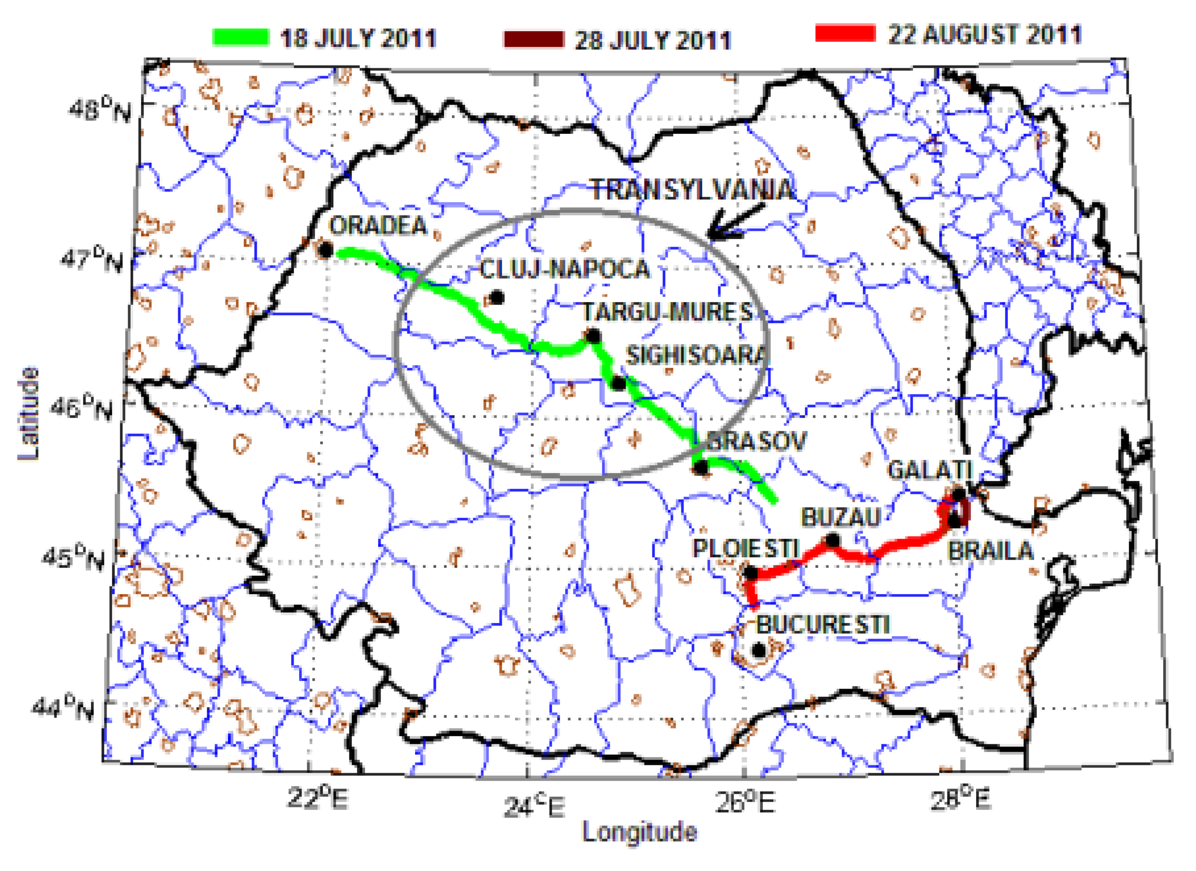
Mobile DOAS zenith-sky measurements were performed in Romania during three days in summer 2011: July 18, July 28 and August 22. The measurements covered about 800 km in different regions of the country, including urban, rural and industrial areas (Figure 1). All measurements were performed under clear sky or mostly clear sky conditions. The time interval of measurements, the distance traveled and the main cities on road route are presented in Table 1.
Besides mobile measurements, a static DOAS experiment took place on 6 October 2011, at twilight-sunrise in a rural area close to Galati city.
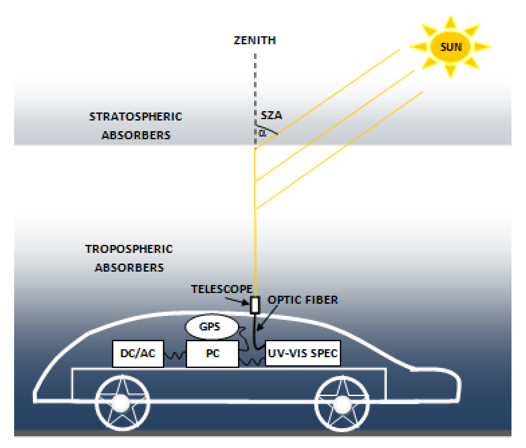
The mobile DOAS instrument used in this work is based on a compact Czerny-Turner spectrometer (AvaSpec 2048 USB2, of 175 × 110 × 44 mm dimensions and 716 g weight) placed in a car. The spectral range of the spectrometer is 200–750 nm with 1.5 nm resolution (FWHM) with a focal length of 75 mm. The entry slit is 50 μm and the grating is 600 L/mm, blazed at 300 nm. The CCD detector is a Sony2048 linear array with a Deep-UV coating for signal enhancement below 350 nm. A flexible device (a piece of wood with a hole cached in a small metallic plate), mounted on the top of the road vehicle, holds the telescope achieving a 1.2° field-of-view with fused silica collimating lenses. The spectrometer is connected to the telescope through a 400 μm chrome plated brass optical fiber. Each spectrum is recorded by a laptop and georeferenced by a GPS receiver. The spectrometer and the GPS receiver are powered by the laptop USB ports. The entire set-up is powered by 12 V of the car through an inverter. Each measurement is a 5-second average of 10 scans accumulations at an integration time between 4–12 ms. The instrument was adapted from an instrument developed at BIRA-IASB [18]. Figure 2 presents the instrumental set-up.
2.2. Determination of Tropospheric Vertical Columns of NO2
The analysis of the zenith-sky spectra was performed using the QDOAS software [26], a program dedicated to the DOAS retrieval of atmospheric trace gases from ground-based and satellite measurements. The NO2 column density was retrieved in the spectral region 425–500 nm where NO2 has strong absorption lines. Absorption of O3, H2O and O4 can also be detected in the same region. The cross sections of NO2 at 298 K and 220 K [27], O3[28], O4 ( http://www.aeronomie.be/spectrolab/o2.htm) and H2O [29] were included in the spectral fitting process. The “Filling-in” effect on Fraunhofer lines, also known as the Ring effect, originating from the rotational Raman scattering of molecular oxygen and nitrogen [30] was corrected by including into the fit a synthetic Ring spectrum calculated with QDOAS. Also a fifth degree polynomial representing the contribution of broad-band absorption in the atmosphere (Rayleigh and Mie scattering) was used in the DOAS analysis. The result of the DOAS fit is a Differential Slant Column Density (DSCD) of NO2 which is the difference between the slant column densities in the measured spectra (SCD) and in the Fraunhofer reference spectrum (SCDref).
In our case, the tropospheric NO2 VCD retrieval from zenith-sky observations, or the mobile DOAS measurement results, involves complementary ground-based and satellite measurements. Determination of the NO2 amount in SCDref is required in order to determine the tropospheric NO2 VCD. Another important parameter is the air mass factor (AMF) which is needed to convert the resulted slant columns to vertical columns. The AMF is defined as the ratio between SCD and VCD (Equation (1)):
The total slant column density in a measured spectrum (SCDmeas) is defined by Equation (2):
Stratospheric and tropospheric content of NO2 contribute to the measured slant column density, according to:
2.2.1. Deduction of SCDref
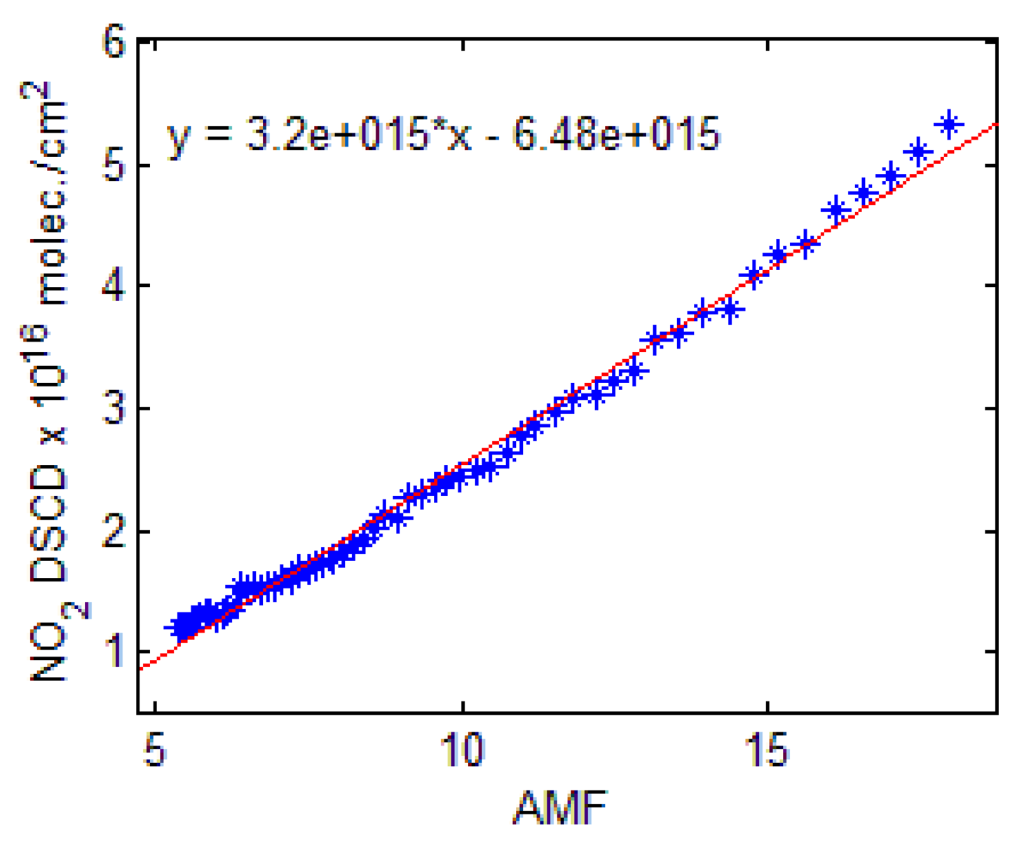
A common way to quantify the SCDref is to use a Langley plot which is the graphical representation of DSCD at twilight versus the associated AMF [31]. By applying a linear fit to the resulting curve the slope gives the VCD and the intercept gives the SCDref, as shown in Equation (5):
For NO2, due to the rapid variation of the NO2 concentration in the stratosphere at twilight, a photo-chemically modified Langley-plot is required [31–33]. We thus used scaled AMFs calculated using the radiative transfer model (RTM) UVspec/DISORT [34] coupled to the photochemical box-model PSCBOX [35–37]. Both box-model and RTM have been validated through several comparison exercises [36–39]. For the present study, the box-model PSCBOX is daily initialized with chemical and meteorological fields extracted from the 3-D chemical transport model (CTM) SLIMCAT [40] for the Jungfraujoch station (46.5°N, 8°E) in Switzerland which is similar in latitude to the locations of the mobile DOAS performed in Romania.
A spectrum with a low NO2 content recorded on 18 July 2011 at 8.82 UT and SZA = 33° was selected to represent and to determine the NO2 amount in the reference spectrum. The reference spectrum was selected after a pre-analysis of DSCDs with a random spectrum. The reference spectrum was recorded in a clean area in forested mountains, Transylvania (46.93°N, 22.83°E). The stratospheric contribution in this spectrum is supposed to be small considering the small SZA. All spectra presented in this paper have been analyzed with this spectrum. The benefits of using a single reference spectrum consist in avoiding different systematic errors which could affect the analysis process [41].
The NO2 amount in the reference spectrum was obtained from ground-based zenith-sky measurements at sunrise on 6 October 2011. Figure 3 shows the photo-chemically corrected Langley plot for the SZA interval 90°–80°. The intercept of the corresponding straight line, representing SCDref and derived by linear least-squares regression, was found to be 6.48 ± 0.36 × 10¹⁵ molec./cm2.
2.2.2. Deduction of VCDstrato
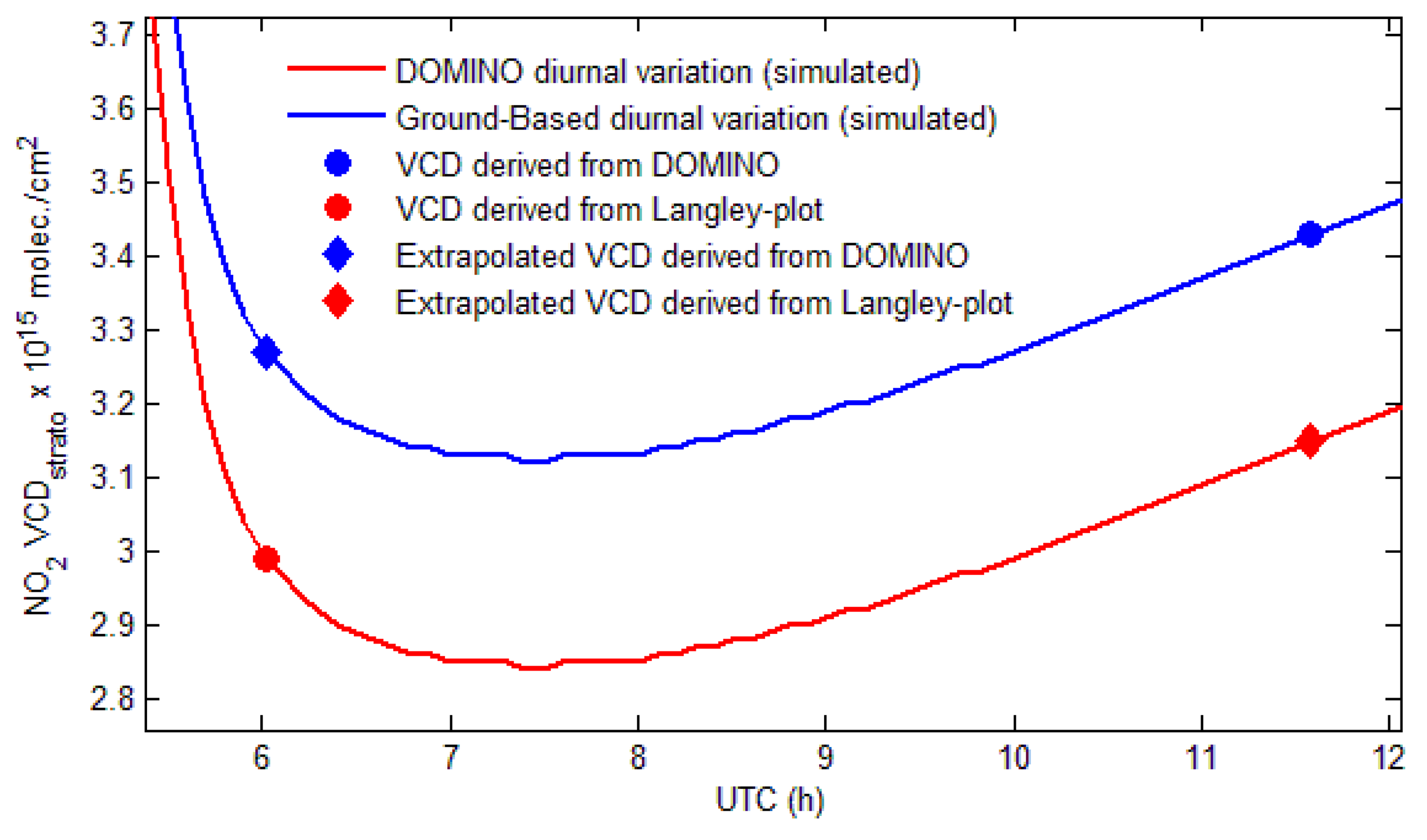
Two methods for the determination of the stratospheric NO2 are described below. The first method is based on the derivation of stratospheric VCDs from measurements at sunrise by using the Langley-plot analysis presented in [42]. The authors used sunrise/sunset observations analyzed with a reference spectrum at 75°SZA (Equation (6)) which ensures that the potential impact of tropospheric NO2 variation in the Langley-plot analysis is reduced. This method can be successfully applied for sunrise/sunset observations performed in less polluted areas. Unfortunately it cannot be used for the retrieval of tropospheric NO2 from our mobile measurements because these were not performed at twilight, but during daytime. However, the above method was used to infer stratospheric content of NO2 using the static DOAS measurements on 6 October 2011. The AM variation of VCDstrato including the sunrise of 6 October 2011 will be estimated by extrapolating the slope resulted from Langley-plot to the simulation of the PSCBOX-model. The VCDstrato for 6 October 2011 was estimated at about 2.99 × 10¹⁵ molec./cm2 (6:18 UTC):
The second method to derive the stratospheric contribution is based on using the stratospheric NO2 columns obtained from the OMI instrument onboard AURA satellite. The assimilated vertical stratospheric columns were extracted from DOMINO (Dutch OMI NO2) Level2 product [43]. The stratospheric NO2 slant column from DOMINO is estimated by data-assimilation of OMI slant columns in TM4 chemistry-transport model. The selection of data satellite was made for an area with a radius with the half linear distance between the first and the last point of ground measurement. Variation of stratospheric NO2 in OMI data over Romania was found less than 5%. Table 2 lists the satellite overpass data sets that were used for the present analysis.
Figure 4 compares the stratospheric VCD derived from the photo-chemically modified Langley-plot and from OMI. The diurnal variation of VCDstrato was calculated by extrapolating data from OMI measurements to the simulation of the PSCBOX model. Stratospheric NO2 columns from the DOMINO retrieval exceed the ground-based measurements by no more than 0.3 × 10¹⁵ molec./cm2. In a recent study [44], where DOMINO was compared with the SAOZ (Système d'Analyse par Observations Zénithal) instruments and the Network for the Detection of Atmospheric Composition Change (NDACC), a similar level of agreement was found.
Both methods presented in this chapter are suitable to retrieve the tropospheric NO2 content but the first method requires observations around twilight which are missing for the days with mobile measurements. Therefore, in this work, the DOMINO-based method was used to estimate stratospheric NO2.
2.2.3. AMFs Simulations
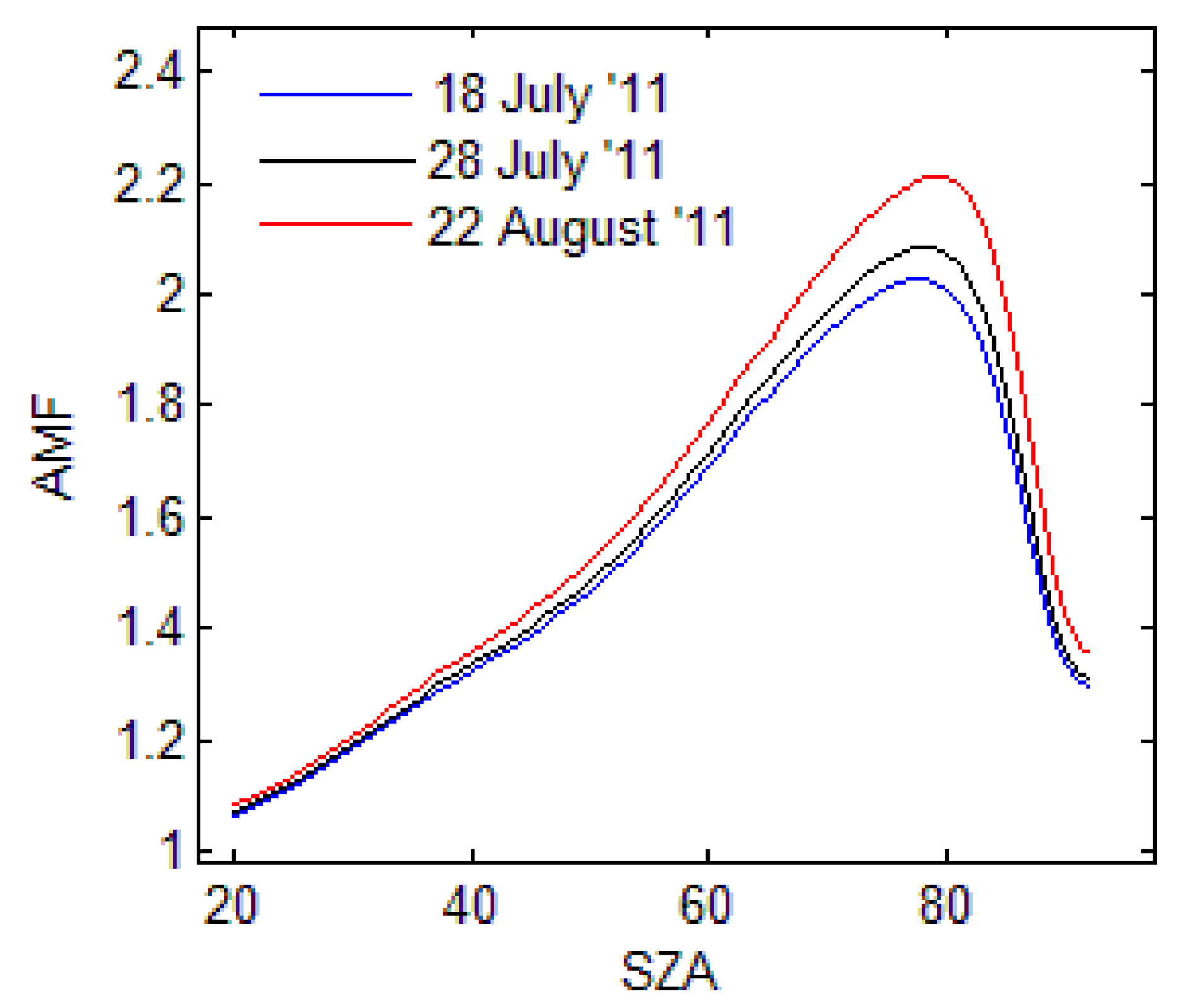
The AMFs simulations presented in this study were performed using the radiative transfer model (RTM) UVspec/DISORT. The RTM is based on the discrete ordinate method and deals with multiple scattering in a pseudo-spherical approximation. Given the wavelength, the observation's geometry relative to the Sun and the atmospheric state, the model calculates the scattered radiance and the absolute SCD of molecular absorbers. For the tropospheric AMF simulations we used NO2 profiles representative of Romania obtained from the CHIMERE model. The AMFtropo simulations were made by setting a grid of 10 km altitude and the wavelength for NO2 simulation at 440 nm. Figure 5 shows the results of tropospheric AMFs simulations for the three days with road measurements in 2011.
3. Results and Discussions
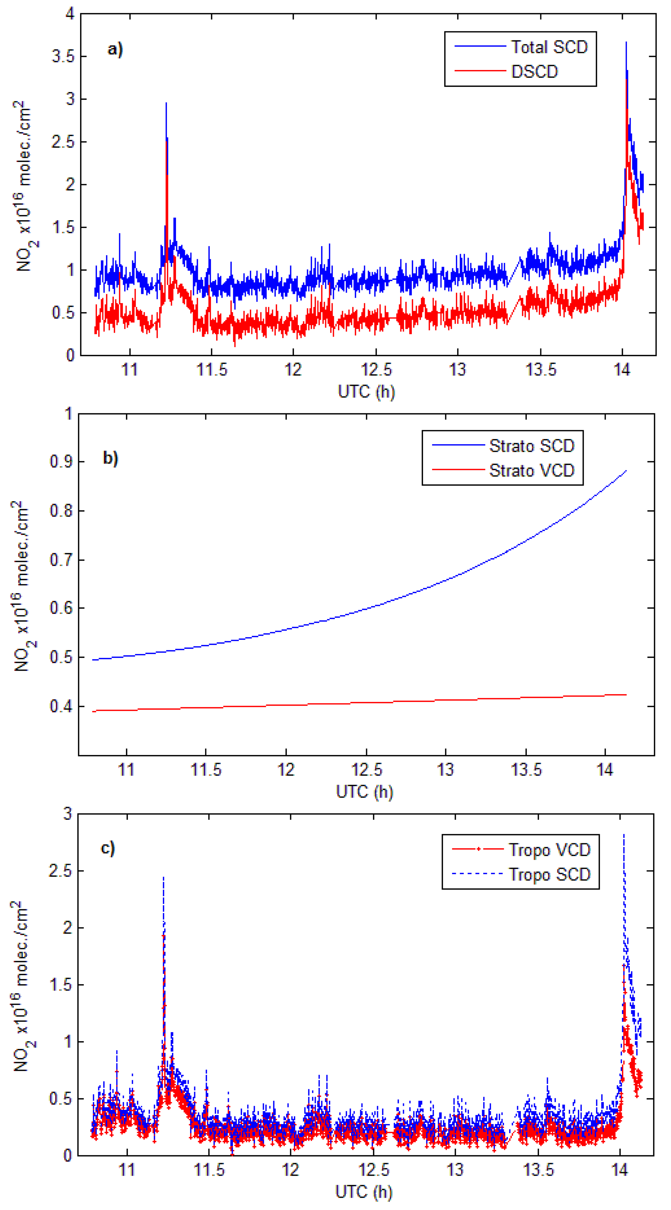
Figure 6 presents the spatial variation of tropospheric NO2 VCDs and the corresponding NO2 slant columns measured on 22 August 2011. The comparison of the DSCD with the VCDtropo gives similar values around noon, which can be explained by the quasi vertical light path of solar photons through the atmosphere when the sun is high. Also this might indicate that a noon reference spectrum with a low NO2 content can correct for stratospheric slant column [42]. After noon, the DSCD increasingly and linearly deviates from the VCDtropo at a rate of approximately 1% per degree of SZA. This is due the diurnal variation of stratospheric NO2.
3.1. Error Estimation
This section presents an analysis of the errors and of their propagation through the retrieval process. Each parameter used in the determination of tropospheric VCD has a contribution to the accuracy of the final retrieval. The error propagation on tropospheric VCD (σVCD) can be expressed by Equation (7):
Note that this expression assumes that the different error sources are uncorrelated, which is justified by the different origins of these error sources, which are described below. A correlation between the error of the DSCDs and the error of SCDref might exist if the NO2 cross section used in the DOAS fit is inaccurate, but this is not seen in our case. The error sources in our calculation are the following:
The error on the DOAS fitting (σDSCD) is calculated by QDOAS software and was found to be generally less than 1 × 10¹⁵ molec./cm2.
The error on the estimation of the slant column in the reference spectra (SCDref), which was obtained using a Langley plots (σSCDref), depends on the one hand on the NO2 variation during twilight and on the other hand on the correct selection of the SZA interval for the AMF calculation used in the Langley plots. In our case, the error on the SCDref was calculated using the standard error formula for the case of simple linear regression.
The selection of an adequate SZA interval for the determination of SCDref is a critical issue. Table 3 shows that different SZA intervals used in the linear fitting may induce different values of intercepts. To rate the different possible choices, we consider the mean squared error (MSE) and the standard error of the linear regression. The interval with the smallest errors was selected as confidently representing the Langley plot. Using SZAs from 90° to 80°, the estimated σSCDref is of 3.56 × 10¹⁴ molec./cm2. As mentioned in Section 2.2.2, the measurements at large SZA are less contaminated by tropospheric NO2, On the other hand, when the sun is under the horizon, the available light is much reduced and the errors on the DOAS fit increase. The interval 90°–80° was chosen since it minimized the fit error.
The error on stratospheric SCD (σSCDstrato) is the uncertainty on the assimilated stratospheric slant column from DOMINO data product v2.0. This error is based on observation-forecast statistics [43–45] and is estimated to be 0.25 × 10¹⁵ molec./cm2.
The AMF calculation can introduce important errors on the retrieval process of tropospheric VCDs. The tropospheric AMFs applied in this work were computed with DISORT using NO2 profiles from the CHIMERE chemistry transport model over Romania. In [46] the AMFtropo uncertainties are estimated at 10%–20%, for SZA increasing from 20° to 85°. They use various input parameters for the radiative transfer simulation. Since their study presents an accurate description of AMF's uncertainties, their estimations of the error on tropospheric AMFs were used here.
After analyzing each error source we find that the major source of error comes from the DOAS fit. Our calculations show that, for all mobile measurements, the typical uncertainty on the retrieved NO2 tropospheric VCD is less than 25%.
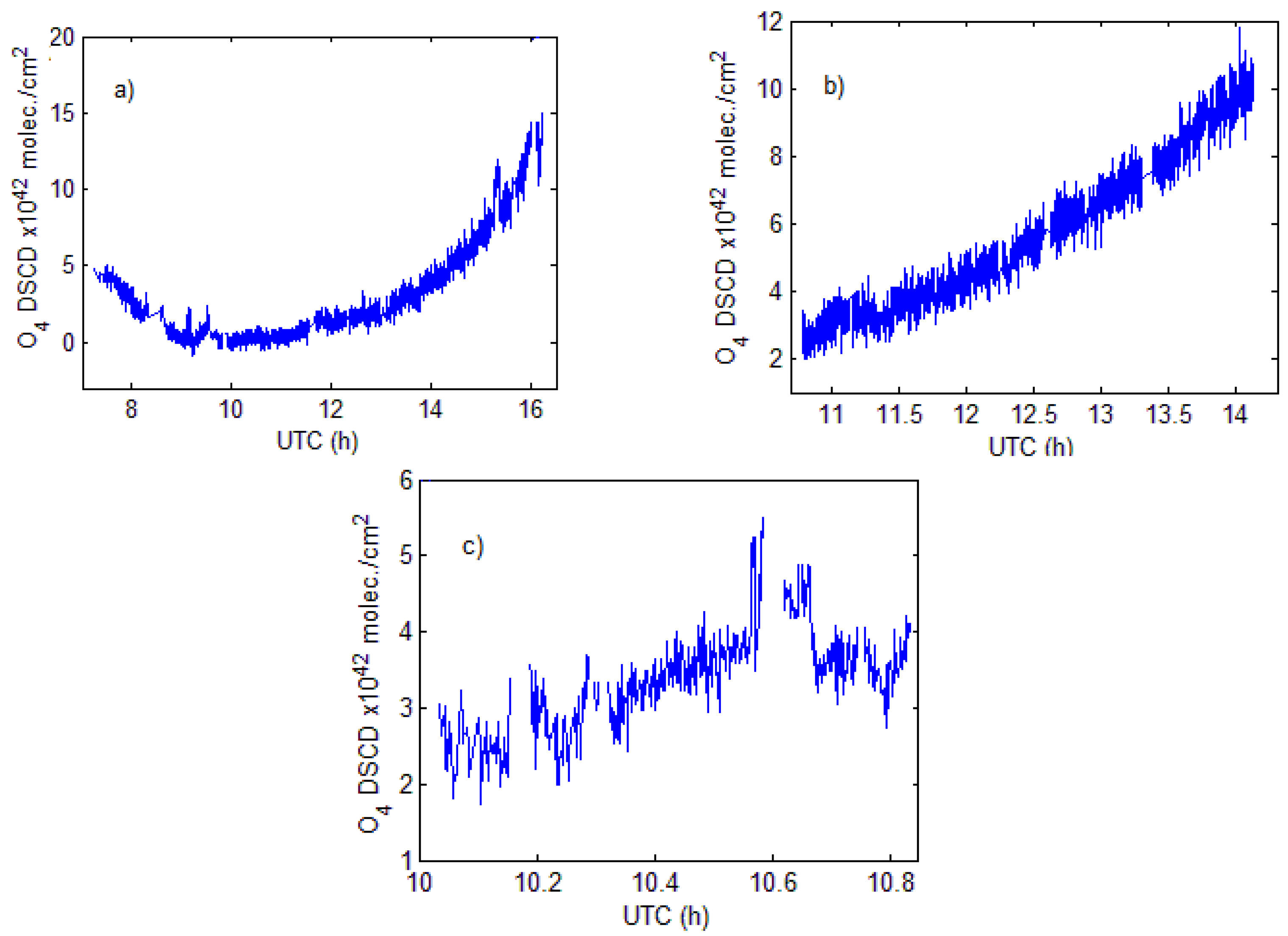
As an additional selection criterion, O4 absorption measurements performed together with NO2 were used as an indicator for the variation of the radiative transport through the atmosphere [47]. In a clear sky atmosphere, the oxygen collisional dimer O4 absorption varies with the square of the oxygen pressure [48] and is weakly dependent on temperature [49]. Analyzing the O4 DSCDs resulting from the DOAS fit (Figure 7) the time variations of O4 can therefore give an idea of the light path enhancement through the atmosphere.
3.2. Comparison of Our Mobile Measurements with Satellite Data
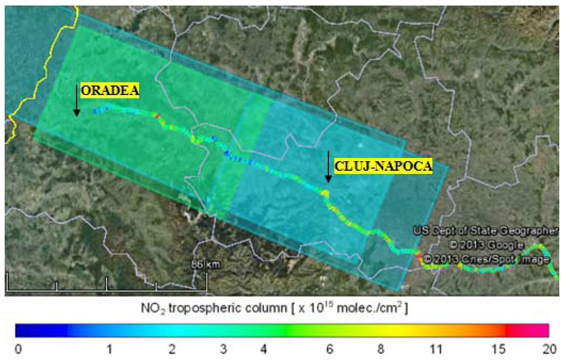
In this section the tropospheric VCDs retrieved from mobile zenith-sky measurements are compared with the tropospheric VCDs derived from the nadir measurements of OMI and GOME-2 instruments, onboard the AURA and Metop-A satellites. Only pixels with the geographic center located below 20 km distance of mobile measurements for GOME-2 and respective 10 km for OMI were selected for comparison. The largest number of mobile measurements were made on 18 July 2011, but they could not be used for comparison with OMI observations because the satellite passed over Romania close to the West border of the country, while the ground measurements were performed inside the country, more than 50 km away from the closest satellite pixel. The only day when matching observations from both satellites exist was 22 August 2011. In Figure 8 a color coded comparison between road measurements and GOME-2 observations made on 18 July 2011 is shown.
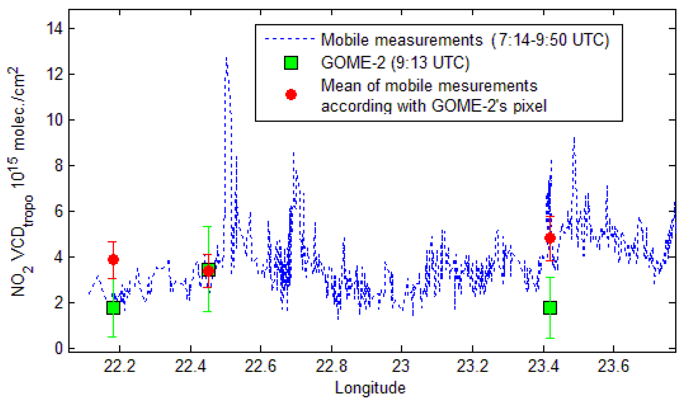
The next figure presents measurements of GOME-2, with a horizontal resolution of 40 × 80 km2, mobile observations and the average of mobile observations according to pixel size of GOME-2. Satellite observations and averages of mobile measurements are accompanied by error bars. The background NO2 satellite loading was considered to be the minimum observed by satellite, which is (1.8 ± 1.3) × 1015 molec/cm2.
The NO2 background for mobile measurements was obtained by averaging the measurements between 22.8 and 23.1 longitude, where NO2 is low and relatively constant. This gives (2.5 ± 0.6) × 1015 molec./cm2 which is close to the minimum observed by satellite.
After averaging the tropospheric NO2 columns along the spatial extent of the satellite pixel, for a location centered on 47.03°N, 22.45°E which is influenced by emissions of two important cities, Oradea (47.05°N, 21.94°E) and Cluj-Napoca (46.76°N, 23.60°E), the NO2 loadings were found to be similar. For this location the averaged mobile measurements amount to (3.4 ± 0.7) × 1015 molec./cm2 while GOME-2 observations indicate (3.4 ± 1.9) × 1015 molec./cm2. Figure 9 shows that satellite measurements in the pixels located at 22.2 and 23.4 longitude are significantly smaller than mobile measurements. The satellite cannot “see” NO2 emissions from very small areas (e.g., NO2 located around to the road with low traffic, small cities or villages) while mobile measurements can determine the NO2 at a very small resolution comparing to GOME-2 observations (40 × 80 km2). The area of measurements is generally “clean” of NO2 being covered mostly by forested mountains. We believe that an increased number of measurements inside the GOME-2 pixels, away from point sources of NO2, would reduce discrepancies after averaging the mobile measurements according to the size of the satellite pixel.
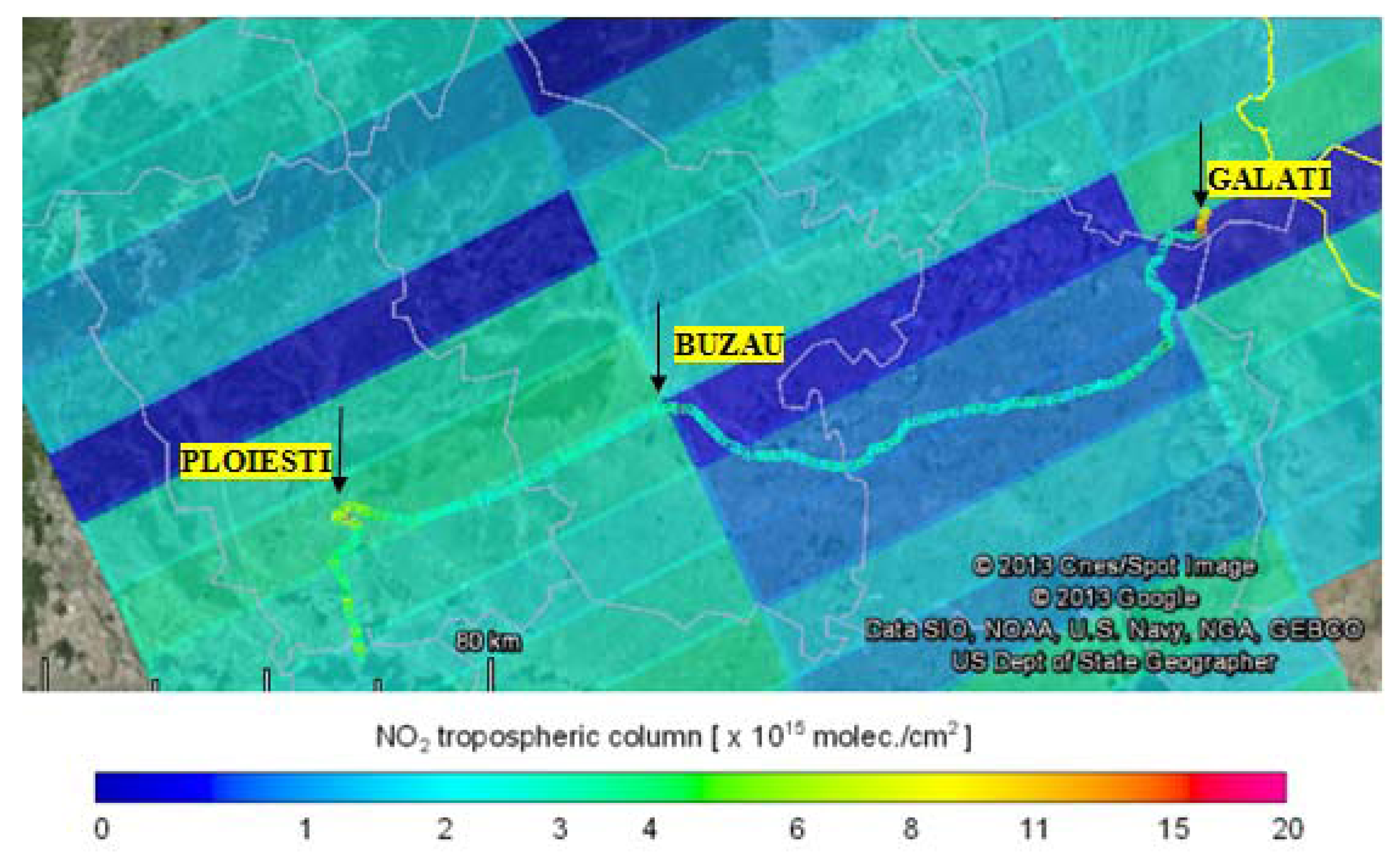
In Figure 10 we present the color coded comparison between road measurements and OMI measurements for another day, 22 August 2011.
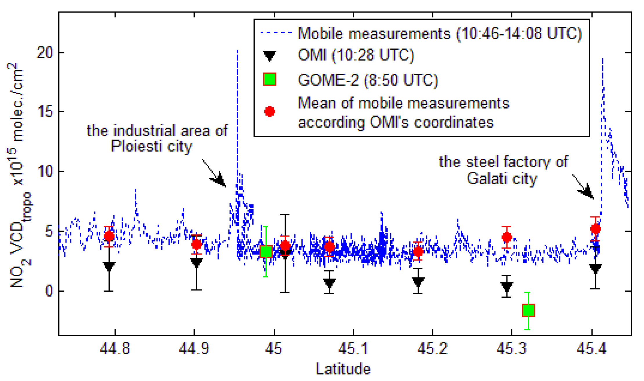
Figure 11 shows the tropospheric NO2 VCD derived from zenith-sky measurements corresponding to OMI and GOME-2 satellite observations, as a function of latitude. The first NO2 peak of mobile measurements was recorded close to a power plant around Ploiesti city and the second one was recorded around a steel and iron factory which is close to the Galati city. Between these cities no other strong source for NO2 emissions exists along the trajectory of the mobile measurements. The NO2 background for mobile measurements is estimated at about (3.5 ± 0.6) × 1015 molec./cm2. The satellite instruments generally underestimate NO2 content, especially in less polluted areas. However, the difference between satellite and mobile observations are reduced in areas where strong NO2 sources are encountered.
The smoothing effect is significant even for OMI measurements with the finest resolution (13 × 24 km2) for areas with localized NO2 sources. For a better comparison we average the ground measurements according to the size of the OMI pixels. This reduces the differences between the two sets of measurements. For instance, at 11:10 UTC, around coordinates 44.9°N, 26.1°E, which corresponds to the industrial area of Ploiesti city, GOME-2 reports a NO2 content of (3.3 ± 2.1) × 1015 molec./cm2, OMI gives (3.2 ± 3.2) × 1015 molec./cm2 and the average of mobile measurements shows (3.8 ± 0.8) × 1015 molec./cm2.
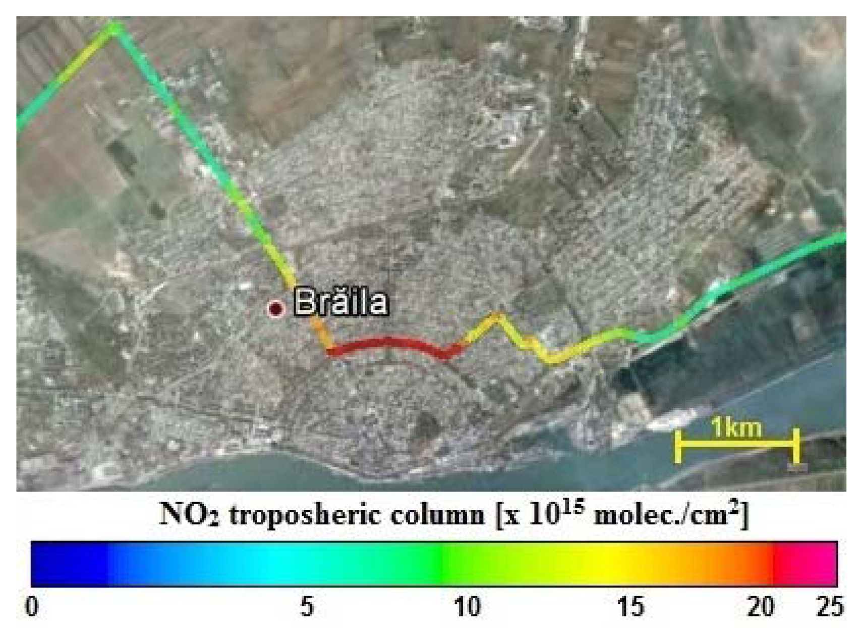
Figure 12 shows a “zoom” inside of an OMI pixel made by mobile DOAS measurements in Braila city on 28 July 2011. Braila city is a relatively small city (77.9 km2), whose main source of atmospheric pollution is due to local transportation. The maximum mobile tropospheric NO2 column recorded is (2.5 ± 0.5) × 1016 molec./cm2 and its corresponding average for an OMI pixel is (4.9 ± 1.2) × 1015 molec./cm2. For the same area, OMI reports a column of about (2.4 ± 1.3) × 1015 molec./cm2. The significant difference between OMI and mobile DOAS measurements is probably caused by the smoothing effect inside the pixel. The total surface of an OMI pixel is 312 km2 which is 4 times larger than the area where local transportation increases the NO2 content. The size of the satellite pixel and the magnitude of the hot-spot are most likely responsible for these discrepancies.
4. Conclusions
Zenith-sky mobile DOAS measurements were performed in Romania over large areas during three days in summer 2011. These were complemented by static measurements at twilight. A detailed method for retrieval of tropospheric NO2 VCDs using ground-based and satellite observations is presented. This method presents three steps. First the NO2 amount in the reference spectrum is determined from ground-based measurements performed at twilight-sunset, using a photo-chemically modified Langley plot. The second step consists in determining the stratospheric NO2 SCD content by means of the assimilated vertical stratospheric column from the satellite DOMINO NO2 product. By comparing stratospheric NO2 VCDs derived from DOMINO with twilight observations for the morning of 6 October 2011, it is found that the stratospheric NO2 from DOMINO exceeds the ground-based measurements by no more than 0.3 × 10¹⁵ molec./cm2. To determine the diurnal variation of stratospheric NO2, PSCBOX model simulations were used. Finally, the tropospheric VCD was determined using a tropospheric AMF calculated with the RTM UVspec/DISORT, using NO2 profiles representative of Romania obtained from the CHIMERE model. Error propagation on tropospheric VCD was estimated to be less than 25%.
The comparison of the mobile DOAS measurements with results of OMI and GOME-2 instruments shows that satellite-based measurements generally underestimate ground based mobile observations for areas with VCD NO2 background smaller than 5 × 10¹⁵ molec./cm2. In contrast, the difference between mobile observations and satellite measurements is reduced in areas with strong NO2 emissions. Averaging mobile measurements in order to better match the horizontal extent of satellite pixels nearby a NO2 pollution source on 18 July 2011 gives (3.4 ± 0.7) × 1015 molec./cm2, while the corresponding result of GOME-2 for the same area gives shows (3.4 ± 1.9) × 1015 molec./cm2. On 22 August 2011, around Ploiesti city (44.99°N, 26.1°E), GOME-2 measures a NO2 content of (3.3 ± 1.9) × 1015 molec./cm2, OMI gives (3.2 ± 3.2) × 1015 molec./cm2 while the corresponding average of mobile measurements is (3.8 ± 0.8) × 1015 molec./cm2. Over “clean areas” with forested mountains, the average of ground measurements on 18 July 2011 gives (2.5 ± 0.6) × 1015 molec./cm2 while the satellite observations show (1.8 ± 1.3) × 1015 molec./cm2.
One of the possible future applications for mobile measurements such as presented in this work would be to derive more accurate NO2 emissions data around point sources. The comparison of mobile measurements with simultaneous Multi-Axis (MAX-) DOAS measurements and satellite observations will be the subject of a future paper.
Acknowledgments
D.E. Constantin's work for this study was supported by the Grant SOP HRD/107/1.5/S/76822 TOP ACADEMIC co financed from ESF of EC, Romanian Government and “Dunarea de Jos” University of Galati, Romania. François Hendrick would like to thank M. P. Chipperfield (University of Leeds, UK) for providing SLIMCAT data. The DOMINO data product was taken from the ESA TEMIS archive ( www.temis.nl) maintained at KNMI, The Netherlands. M. Voiculescu was partly supported by project PN-II-ID-PCE-2011-3-0709, SOLACE of the Romanian NPRDI-II, UEFISCDI.
References
- Crutzen, P.J. The influence of nitrogen oxides on the atmospheric ozone content. Q. J. R. Meteorol. Soc. 1970, 96, 320–325. [Google Scholar]
- Solomon, S.; Portmann, R.W.; Sanders, R.W.; Daniel, J.S.; Madsen, W.; Bartram, B.; Dutton, E.G. On the role of nitrogen dioxide in the absorption of solar radiation. J. Geophys. Res. 1999, 104, 12047–12058. [Google Scholar]
- Lee, D.S.; Köhler, I.; Grobler, E.; Rohrer, F.; Sausen, R.; Gallardo-Klenner, L.; Olivier, J.G.J.; Dentener, F.J.; Bouwman, A.F. Estimations of global NOx emissions and their uncertainties. Atmos. Environ. 1997, 31, 1735–1749. [Google Scholar]
- Beirle, S.; Platt, U.; Wenig, M.; Wagner, T. Weekly cycle of NO2 by GOME measurements: A signature of anthropogenic sources. Atmos. Chem. Phys. 2003, 3, 2225–2232. [Google Scholar]
- Sunyer, J.; Spix, C.; Quenel, P.; Ponce-de-Leon, A.; Ponka, A.; Barumandzadeh, T.; Touloumi, G.; Bacharova, L.; Wojtyniak, B.; Vonk, J.; et al. Urban air pollution and emergency admissions for asthma in four European cities: The APHEA Project. Thorax 1997, 52, 760–765. [Google Scholar]
- Maître, A.; Bonneterre, V.; Huillard, L.; Sabatier, P.; de Gaudemaris, R. Impact of urban atmospheric pollution on coronary disease. Eur. Heart J. 2006, 27, 2275–2284. [Google Scholar]
- van der A, R.J.; Peters, D.H.M.U.; Eskes, H.; Boersma, K.F.; van Roozendael, M.; De Smedt, I.; Kelder, H.M. Detection of the trend and seasonal variation in tropospheric NO2 over China. J. Geophys. Res. 2006, 111, D12317. [Google Scholar]
- Platt, U. Differential optical absorption spectroscopy (DOAS). Chem. Anal. Ser. 1994, 127, 27–83. [Google Scholar]
- Platt, U.; Stutz, J. Differential Optical Absorption Spectroscopy: Principles and Applications; Springer Verlag: Heidelberg, Germany, 2008. [Google Scholar]
- Brewer, A.W.; McElroy, C.T.; Kerr, J.B. Nitrogen dioxide concentration in the atmosphere. Nature 1973, 246, 129–133. [Google Scholar]
- Noxon, J.F. Nitrogen dioxide in the stratosphere and troposphere measured by ground-based absorption spectroscopy. Science 1975, 189, 547–549. [Google Scholar]
- Johansson, M.; Galle, B.; Yu, T.; Tang, L.; Chen, D.; Li, H.; Li, J.X.; Zhang, Y. Quantification of total emission of air pollutants from Beijing using mobile mini-DOAS. Atmos. Environ. 2008, 42, 6926–6933. [Google Scholar]
- Johansson, M.; Rivera, C.; de Foy, B.; Lei, W.; Song, J.; Zhang, Y.; Galle, B.; Molina, L. Mobile mini-DOAS measurement of the outflow of NO2 and HCHO from Mexico City. Atmos. Chem. Phys. 2009, 9, 5647–5653. [Google Scholar]
- Rivera, C.; Sosa, G.; Wöhrnschimmel, H.; de Foy, B.; Johansson, M.; Galle, B. Tula industrial complex (Mexico) emissions of SO2 and NO2 during the MCMA 2006 field campaign using a mobile mini-DOAS system. Atmos. Chem. Phys. 2009, 9, 6351–6361. [Google Scholar]
- Rivera, C.; Mellqvist, J.; Samuelsson, J.; Lefer, B.; Alvarez, S.; Patel, M.R. Quantification of NO2 and SO2 emissions from the Houston Ship Channel and Texas City industrial areas during the 2006 Texas Air Quality Study. J. Geophys. Res. 2010, 115, D08301. [Google Scholar]
- Strong, K.; Bailak, G.; Barton, D.; Bassford, M.; Blatherwick, R.; Brown, S.; Chartrand, D.; Davies, J.; Fogal, P.; Forsberg, E.; et al. Mantra—A balloon mission to study the odd-nitrogen budget of the stratosphere. Atmos. Ocean 2005, 43, 283–299. [Google Scholar]
- Bossmeyer, J. Ship-Based Multi-Axis Differential Optical Absorption Spectroscopy Measurements of Tropospheric Trace Gases over the Atlantic Ocean—New Measurement Concepts. PhD Thesis, Institut fur Umweltphysik, University of Heidelberg, Heidelberg, Germany, 2002. [Google Scholar]
- Merlaud, A.; van Roozendael, M.; Theys, N.; Fayt, C.; Hermans, C.; Quennehen, B.; Schwarzenboeck, A.; Ancellet, G.; Pommier, M.; Pelon, J.; et al. Airborne DOAS measurements in Arctic: Vertical distributions of aerosol extinction coefficient and NO2 concentration. Atmos. Chem. Phys. 2011, 11, 9219–9236. [Google Scholar]
- Merlaud, A.; van Roozendael, M.; van Gent, J.; Fayt, C.; Maes, J.; Toledo-Fuentes, X.; Ronveaux, O.; de Mazière, M. DOAS measurements of NO2 from an ultralight aircraft during the Earth Challenge expedition. Atmos. Meas. Tech. 2012, 5, 2057–2068. [Google Scholar]
- Bovensmann, H.; Burrows, J.P.; Buchwitz, M.; Frerick, J.; Noël, S.; Rozanov, V.V.; Chance, K.V.; Goede, A.H.P. SCIAMACHY—Mission objectives and measurement modes. J. Atmos. Sci. 1999, 56, 127–150. [Google Scholar]
- Levelt, P.; van den Oord, G.; Dobber, M.; Malkki, A.; Visser, H.; de Vries, J.; Stammes, P.; Lundell, J.; Saari, H. Theozone monitoring instrument. IEEE Trans. Geosci. Remote 2006, 44, 1093–1101. [Google Scholar]
- Munro, R.; Eisinger, M.; Anderson, C.; Callies, J.; Corpaccioli, E.; Lang, R.; Lefebvre, A.; Livschitz, Y.; Albinana, A.P. GOME-2 on MetOp. Proceedings of The 2006 EUMETSAT Meteorological Satellite Conference, Helsinki, Finland, 12– 16 June 2006; EUMETSAT P. p. 48.
- Boersma, K.F.; Jacob, D.J.; Trainic, M.; Rudich, Y.; de Smedt, I.; Dirksen, R.; Eskes, H.J. Validation of urban NO2 concentrations and their diurnal and seasonal variations observed from the SCIAMACHY and OMI sensors using in situ surface measurements in Israeli cities. Atmos. Chem. Phys. 2009, 9, 3867–3879. [Google Scholar]
- Wagner, T.; Ibrahim, O.; Shaiganfar, R.; Platt, U. Mobile MAX-DOAS observations of tropospheric trace gases. Atmos. Meas. Tech. 2010, 3, 129–140. [Google Scholar]
- Ibrahim, O.; Shaiganfar, R.; Sinreich, R.; Stein, T.; Platt, U.; Wagner, T. Car MAX-DOAS measurements around entire cities: Quantification of NOx emissions from the cities of Mannheim and Ludwigshafen (Germany). Atmos. Meas. Tech. 2010, 3, 709–721. [Google Scholar]
- Fayt, C.; de Smedt, I.; Letocart, V.; Merlaud, A.; Pinardi, G.; van Roozendael, M. QDOAS Software User Manual; Belgian Institute for Space Aeronomy: Brussels, Belgium, 2011. [Google Scholar]
- Vandaele, A.; Hermans, C.; Simon, P.; Carleer, M.; Colin, R.; Fally, S.; Mérienne, F.; Jenouvrier, A.; Coquart, B. Measurements of the NO2 absorption cross-section from 42,000 cm−1 to 10,000 cm−1 (238–1,000 nm) at 220 K and 294 K (220 K). J. Quant. Spectrosc. Radiat. Transf. 1998, 59, 171–184. [Google Scholar]
- Burrows, J.P.; Richter, A.; Dehn, A.; Deters, B.; Himmelmann, S.; Orphal, J. Atmospheric remote-sensing reference data from GOME—Part 2. Temperature-dependent absorption cross sections of O3 in the 231–794 nm range. J. Quant. Spectrosc. Radiat. Transf. 1999, 61, 509–517. [Google Scholar]
- Coheur, P.; Fally, S.; Carleer, M.; Clerbaux, C.; Colin, R.; Jenouvrier, A.; Mérienne, M.; Hermans, C.; Vandaele, A. New water vapor line parameters in the 26,000–13,000 cm−1 region. J. Quant. Spectrosc. Radiat. Transf. 2002, 74, 493–510. [Google Scholar]
- Grainger, J.F.; Ring, J. Anomalous Fraunhofer line profiles. Nature 1962, 193, 762. [Google Scholar]
- Vaughan, G.; Quinn, P.T.; Green, A.C.; Bean, J.; Roscoe, H.K.; van Roozendael, M.; Goutail, F. SAOZ measurements of stratospheric NO2 at Aberystwyth. J. Environ. Monit. 2006, 8, 353–361. [Google Scholar]
- Lee, A.M.; Roscoe, H.K.; Oldham, D.J.; Squires, J.A.C.; Sarkissian, A.; Pommereau, J.-P. Improvements to the accuracy of zenith-sky measurements of NO2 by visible spectrometers. J. Quant. Spectrosc. Radiat. Transf. 1994, 52, 649–657. [Google Scholar]
- Roscoe, H.K.; Charlton, A.J.; Fish, D.J.; Hill, J.G.T. Improvements to the accuracy of measurements of NO2 by zenith-sky visible spectrometers II: Errors in zero using a more complete chemical model. J. Quant. Spectrosc. Radiat. 2001, 68, 337–349. [Google Scholar]
- Mayer, B.; Kylling, A. Technical note: The libRadtran software package for radiative transfer calculations—Description and examples of use. Atmos. Chem. Phys. 2005, 5, 1855–1877. [Google Scholar]
- Errera, Q.; Fonteyn, D. Four-dimensional variationalchemical assimilation of CRISTA stratospheric measurements. J. Geophys. Res. 2001, 106, 12253–12265. [Google Scholar]
- Hendrick, F.; Mueller, R.; Sinnhuber, B.-M.; Bruns, M.; Burrows, J.P.; Chipperfield, M.P.; Fonteyn, D.; Richter, A.; van Roozendael, M.; Wittrock, F. Simulation of BrO Diurnal Variation and BrO Slant Columns: Intercomparison Exercise between Three Model Packages. Proceedings of the 5th European Workshop on Stratospheric Ozone 2000, Saint Jean de Luz, France, 27 September– 1 October 1999.
- Hermans, C.; Lambert, J.-C.; Pfeilsticker, K.; Pommereau, J.-P. Retrieval of nitrogen dioxide stratospheric profiles from ground-based zenith-sky UV-visible observations: Validation of the technique through correlative comparisons. Atmos. Chem. Phys. 2004, 4, 2091–2106. [Google Scholar]
- Hendrick, F.; van Roozendael, M.; Kylling, A.; Petritoli, A.; Rozanov, A.; Sanghavi, S.; Schofield, R.; von Friedeburg, C.; Wagner, T.; Wittrock, F.; et al. Intercomparison exercise between different radiative transfer modelsused for the interpretation of ground-based zenith-sky and multiaxis DOAS observations. Atmos. Chem. Phys. 2006, 6, 93–108. [Google Scholar]
- Wagner, T.; Burrows, J.P.; Deutschmann, T.; Dix, B.; von Friedeburg, C.; Frieß, U.; Hendrick, F.; Heue, K.-P.; Irie, H.; Iwabuchi, H.; et al. Comparison of box-air-mass-factors and radiances for multiple-axis differential optical absorption spectroscopy (MAX-DOAS) geometries calculated from different UV/visible radiative transfer models. Atmos. Chem. Phys. 2007, 7, 1809–1833. [Google Scholar]
- Chipperfield, M.P. Multiannual simulations with a three-dimensionalchemical transport model. J. Geophys. Res. 1999, 104, 1781–1805. [Google Scholar]
- Bassford, M.R.; Strong, K.; McLinden, C.A.; McElroy, T.C. Ground-based measurements of ozone and NO2 during mantra 1998 using a zenith-sky spectrometer. Atmos. Ocean 2005, 43, 325–338. [Google Scholar]
- Hendrick, F.; van Roozendael, M.; Chipperfield, M.P.; Dorf, M.; Goutail, F.; Yang, X.; Fayt, C.; Hermans, C.; Pfeilsticker, K.; Pommereau, J.-P.; et al. Retrieval of stratospheric and tropospheric BrO profiles and columns using ground-based zenith-sky DOAS observations at Harestua, 60° N. Atmos. Chem. Phys. 2007, 7, 4869–4885. [Google Scholar]
- Boersma, K.F.; Eskes, H.J.; Veefkind, J.P.; Brinksma, E.J.; van der A, R.J.; Sneep, M.; van den Oord, G.H.J.; Levelt, P.F.; Stammes, P.; Gleason, J.F.; Bucsela, E.J. Near-real timeretrieval of tropospheric NO2 from OMI. Atmos. Chem. Phys. 2007, 7, 2103–2118. [Google Scholar]
- Dirksen, R.J.; Boersma, K.F.; Eskes, H.J.; Ionov, D.V.; Bucsela, E.J.; Levelt, P.F.; Kelder, H.M. Evaluation of stratospheric NO2 retrieved from the Ozone Monitoring Instrument: intercomparison, diurnal cycle and trending. J. Geophys. Res. 2011, 116, D08305. [Google Scholar]
- Boersma, K.F.; Eskes, H.J.; Brinksma, E.J. Error analysis for tropospheric NO2 retrieval from space. J. Geophys. Res. 2004, 109, D04311. [Google Scholar]
- Chen, D.; Zhou, B.; Beirle, S.; Chen, L.M.; Wagner, T. Tropospheric NO2 column densities deduced from zenith-sky DOAS measurements in Shanghai, China, and their application to satellite validation. Atmos. Chem. Phys. 2009, 9, 3641–3662. [Google Scholar]
- Wagner, T.; von Friedeburg, C.; Wenig, M.; Otten, C.; Platt, U. UV/Vis observations of atmospheric O4 absorptions using direct moon light and zenith scattered sunlight under clear and cloudy sky conditions. J. Geophys. Res. 2002, 107. [Google Scholar] [CrossRef]
- Janssen, J. Sur les spectres d'absorption de l'oxygene, C. R (in French). Hebd. Seances Acad. Sci. 1886, 102, 1352–1353. [Google Scholar]
- Greenblatt, G.D.; Orlando, J.J.; Burkholder, J.B.; Ravishankara, A.R. Absorption measurements of oxygen between 330 and 1140 nm. J. Geophys. Res. 1990, 95, 18577–18582. [Google Scholar]


| Day | Time Interval UT | Distance Traveled | Main Cities on Road Route |
|---|---|---|---|
| 18 July 2011 | 7.23–16.22 h | 500 km | Oradea (47.05°N, 21.94°E) |
| Cluj-Napoca (46.76°N, 23.60°E) | |||
| Targu Mures (46.54°N, 24.55°E) | |||
| Sighisoara (47.05°N, 21.94°E) | |||
| Brasov (45.65°N, 25.60°E) | |||
| 28 July 2011 | 9.99–10.84 h | 30 km | Galati (45.43°N, 28.03°E) |
| Braila (45.26°N, 27.95°E) | |||
| 22 August 2011 | 10.78–14.12 h | 250 km | Ploiesti (44.94°N, 26.03°E) |
| Buzau (45.15°N, 26.81°E) | |||
| Braila (45.26°N, 27.95°E) | |||
| Galati (45.43°N, 28.03°E) | |||
| Day | Orbite Nr. | Overpass Time | Stratospheric VCD |
|---|---|---|---|
| 18 July 2011 | 37,628 | 11:35 UT | 4.49 × 10¹⁵ molec./cm2 |
| 28 July 2011 | 37,778 | 10:34 UT | 3.96 × 10¹⁵ molec./cm2 |
| 22 August 2011 | 37,413 | 12:05 UT | 4.03 × 10¹⁵ molec./cm2 |
| 6 October 2011 | 38,433 | 11:35 UT | 3.39 × 10¹⁵ molec./cm2 |
| SZA | 92°–80° | 91.5°–80° | 90°–80° | 91.5°–75° | 91.5°–72° | 90°–75° |
|---|---|---|---|---|---|---|
| Intercept (×1015) | −9.98 | −8.51 | −6.48 | −5.77 | −5.07 | −4.31 |
| MSE (×1015) | 2.36 | 1.51 | 0.89 | 1.74 | 1.75 | 1.10 |
| σSCDref(×1014) | 7.13 | 4.80 | 3.56 | 3.75 | 7.13 | 5.09 |
© 2013 by the authors; licensee MDPI, Basel, Switzerland. This article is an open access article distributed under the terms and conditions of the Creative Commons Attribution license (http://creativecommons.org/licenses/by/3.0/).
Share and Cite
Constantin, D.-E.; Merlaud, A.; Van Roozendael, M.; Voiculescu, M.; Fayt, C.; Hendrick, F.; Pinardi, G.; Georgescu, L. Measurements of Tropospheric NO2 in Romania Using a Zenith-Sky Mobile DOAS System and Comparisons with Satellite Observations. Sensors 2013, 13, 3922-3940. https://doi.org/10.3390/s130303922
Constantin D-E, Merlaud A, Van Roozendael M, Voiculescu M, Fayt C, Hendrick F, Pinardi G, Georgescu L. Measurements of Tropospheric NO2 in Romania Using a Zenith-Sky Mobile DOAS System and Comparisons with Satellite Observations. Sensors. 2013; 13(3):3922-3940. https://doi.org/10.3390/s130303922
Chicago/Turabian StyleConstantin, Daniel-Eduard, Alexis Merlaud, Michel Van Roozendael, Mirela Voiculescu, Caroline Fayt, François Hendrick, Gaia Pinardi, and Lucian Georgescu. 2013. "Measurements of Tropospheric NO2 in Romania Using a Zenith-Sky Mobile DOAS System and Comparisons with Satellite Observations" Sensors 13, no. 3: 3922-3940. https://doi.org/10.3390/s130303922