Theoretical Analysis of Interferometer Wave Front Tilt and Fringe Radiant Flux on a Rectangular Photodetector

Abstract
: This paper is a theoretical analysis of mirror tilt in a Michelson interferometer and its effect on the radiant flux over the active area of a rectangular photodetector or image sensor pixel. It is relevant to sensor applications using homodyne interferometry where these opto-electronic devices are employed for partial fringe counting. Formulas are derived for radiant flux across the detector for variable location within the fringe pattern and with varying wave front angle. The results indicate that the flux is a damped sine function of the wave front angle, with a decay constant of the ratio of wavelength to detector width. The modulation amplitude of the dynamic fringe pattern reduces to zero at wave front angles that are an integer multiple of this ratio and the results show that the polarity of the radiant flux changes exclusively at these multiples. Varying tilt angle causes radiant flux oscillations under an envelope curve, the frequency of which is dependent on the location of the detector with the fringe pattern. It is also shown that a fringe count of zero can be obtained for specific photodetector locations and wave front angles where the combined effect of fringe contraction and fringe tilt can have equal and opposite effects. Fringe tilt as a result of a wave front angle of 0.05° can introduce a phase measurement difference of 16° between a photodetector/pixel located 20 mm and one located 100 mm from the optical origin.1. Introduction
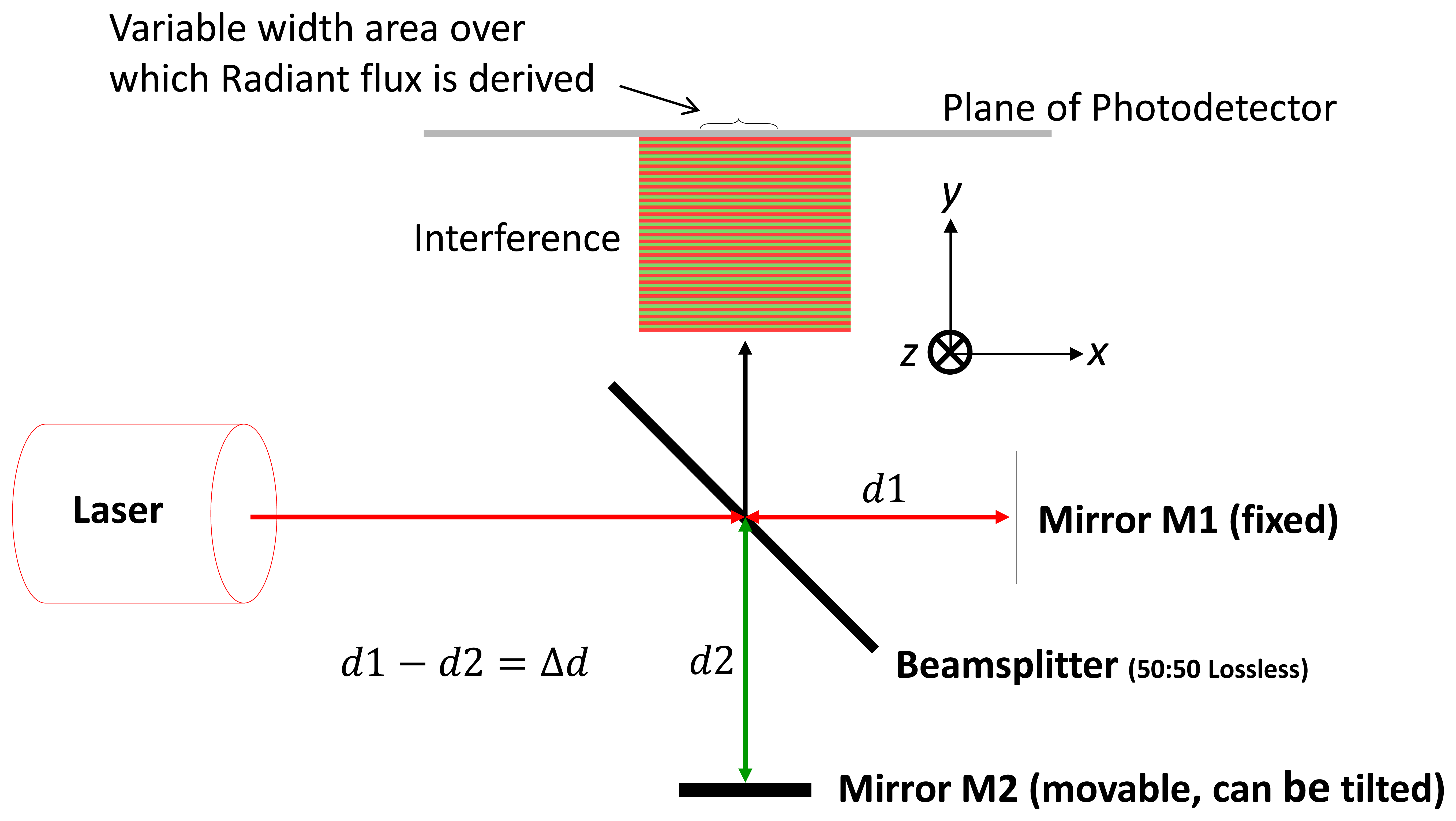
The Michelson interferometer [1] shown in Figure 1 has been used extensively in the field of metrology, most famously in the Michelson-Morley experiment [2]. The measurement is based on detecting and measuring the number of complete and partial fringes resulting from translation of one of the reflecting mirrors and relating the result to the light-source wavelength.
Discrete photodetectors and image sensors are commonly used to detect the sinusoidal pulsing fringe pattern. The radiant flux of the fringe pattern incident on the device active area is mathematically derived by integrating the irradiance over the circular aperture of the light source [3]; over a circular aperture of the interferogram [4–10]; over a square/rectangular aperture of the interferogram [8,11]. Effectively, the active area of the photodetector performs the same function on the irradiance giving an output proportional to the radiant flux.
When using a well collimated beam and plane flat mirrors that are not perfectly aligned, i.e., tilted, fringe lines of equal inclination, width and spacing are produced that contract as the tilt angle is increased and expand as the tilt angle is reduced, having a significant effect on the radiant flux over the active area. This change in radiant flux can be a source of measurement error [3–9] when unconsidered in applications [12–16].
As wave front angle increases, the modulation amplitude of the dynamic fringing reduces and at a specific tilt angle the modulation amplitude of the radiant flux becomes zero [3,5–11,17]. The modulation amplitude is found to decay as a cardinal sine function with a rate of decay proportional to the area of the photodetector and inversely proportional to wavelength.
To overcome or minimise mirror tilt prevalent with flat plane mirrors, corner cube retro-reflectors [8,9], cat-eye reflectors [18] or alternate interferometers [11] are used.
The behaviour of the radiant flux with varying wave front angle is also affected with varying photodetector distance from the central axis of the interferometer and varying its distance from the optical model origin. Analysis of the radiant flux with varying wave front in conjunction with photodetector area, distance from beam centre, distance from origin and wavelength appears not to be covered in the literature although [17] has included distance of the photodetector from the optical model origin specifically to determine the maximum offset angle for a beam-tilting spatial modulation interferometer.
Despite modulation amplitude vs. wave front angle being well understood, to the best of our knowledge, the following analysis is not covered in the literature, i.e., the behaviour of the radiant flux: for a rectangular aperture for varying wave front angle beyond the first modulation zero; over varying active area widths for varying distances from beam centre, e.g., row of pixels across an image sensor; for varying active widths and distances from the tilted mirror; with fringe contraction speed and mirror tilt; with decay constant.
This paper addresses these issues, specifically:
Behaviour of the radiant flux for variable wave front angle as a function of photodetector width and position within the fringe pattern;
Behaviour of the radiant flux on two identical photodetectors adjacent each other;
Magnitude of the radiant flux at wave front angle(s) of equal radiant flux;
Polarity reversal of the radiant flux beyond specific wave front angles;
Behaviour of the radiant flux for variable wave front angle with variable distance of the photodetector from the tilting mirror;
Speed of transition of the fringe lines across the photodetector for variable wave front angle;
Speed of fringe line tilt across the photodetector for variable wave front angle;
Damping function constant of the radiant flux for variable wave front angle.
The relevance of this theoretical analysis is to make evident how these other factors may have an undesirable effect on sensor applications using homodyne interferometry where photodetectors or image sensors are employed to sense small fractions of a fringe to achieve extremely high resolutions of measurement. It goes beyond the adverse effect of modulation amplitude reduction due to increasing wave front angle [3,5–11,17] and introduces what have been termed primary nodes. The results from the mathematical analysis describes how the radiant flux behaves when the five parameters; wave front angle, wave length, photodetector width and position (x, y) are varied independently and concurrently, and how this behaviour can introduce fringe counting errors.
2. Mathematical Analysis
The analysis is carried out based on a conventional Michelson Interferometer that is configured as shown in Figure 1 with the following configuration constraints:
Light source is a collimated monochromatic beam;
Wave fronts over the area of the photodetector are approximated to be plane waves;
Flat plane mirrors are used to reflect the transmitted and reflected beams back to the beamsplitter;
Beamsplitter is lossless and is non-polarising and creates a transmitted and reflected beam of equal amplitude.
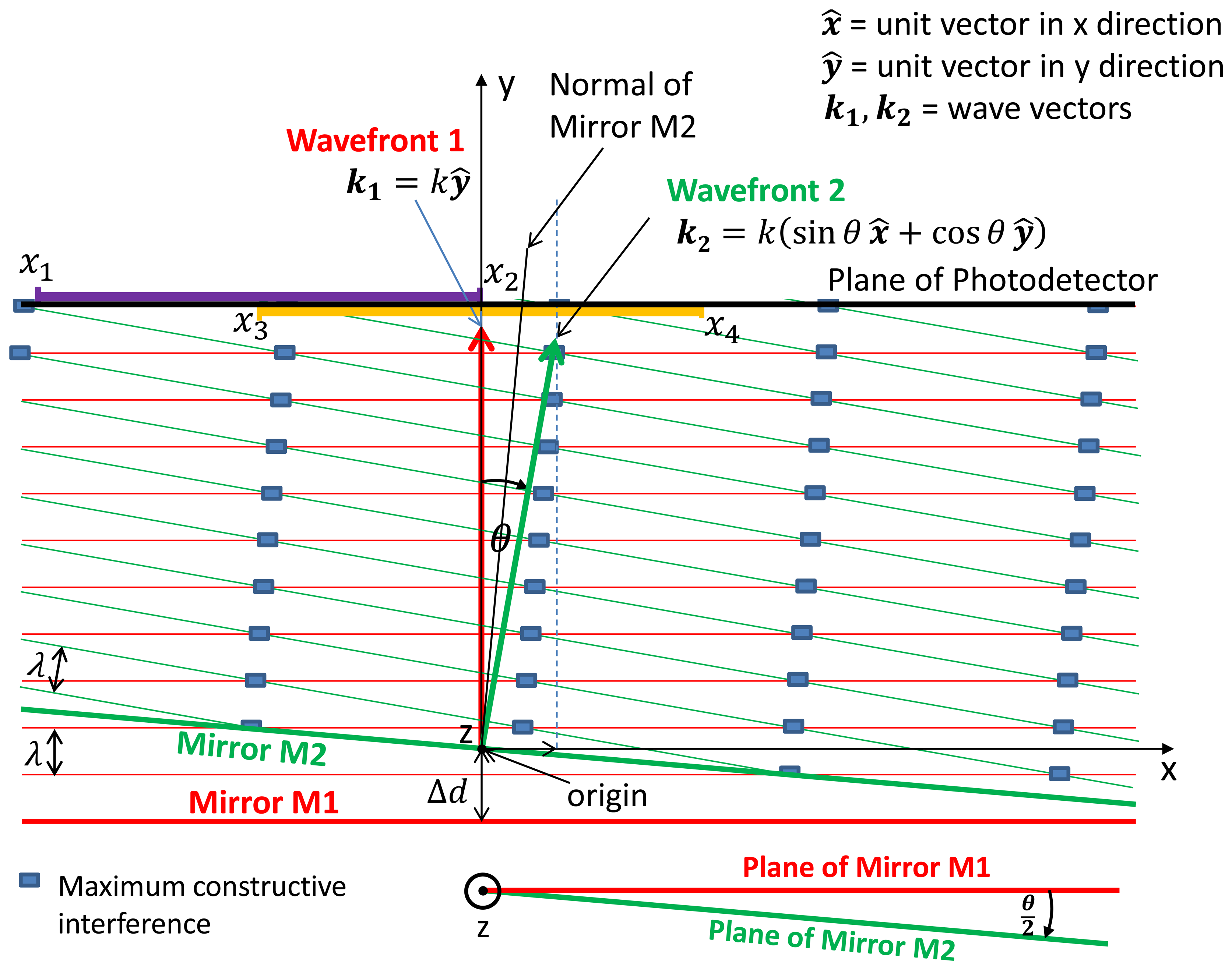
The two wave fronts are orientated as depicted in Figure 2 and all calculations are based on the following constraints:
y axis is taken to be normal to wave front 1;
Origin of the Cartesian coordinate system is the point at which the centre of the incident beam is reflected by mirror M2;
Mirror M2 tilts only about the z-axis;
Mirror M2 translates only along the y-axis;
Plane of the photodetector remains orthogonal to the y axis;
Shape of the active area of the photodetector is rectangular with variable side length s in the x direction and fixed side length z (set to unity) in the z direction;
Fringe pattern irradiates the entire active area of the photodetector;
Output of the photodetector is assumed to be a 1:1 linear function of the incident radiant flux;
Distance to the photodetector from mirror M2 is variable.
The mathematical analysis is divided into the following subsections, the outcome of which is studied further in the Results section:
Derivation of the equation for radiant flux from irradiance of the fringe pattern;
Identification of specific wave front angles θn with invariable radiant flux for two displaced photodetectors of equal size active areas;
Determination of the magnitude of the radiant flux at specific wave front angles θn;
Determination of the linear equation defining the profile of the fringe pattern in the x-y plane;
Determination of the speed of the fringe lines with variable wave front angle θ;
Determination of the damping function of the radiant flux with variable wave front angle θ.
Note: The angle θ in this paper refers to the angle that Wave Front 2 makes with Wave Front 1. The tilt angle of Mirror M2 is therefore θ/2 relative to Mirror M1.
2.1. Derivation of the Equation for Radiant Flux
The electric field of a plane wave is given by Equation (1) [19]:
Figure 2 depicts the linear optical equivalent of the Michelson interferometer with the virtual source wave front approaching mirrors M1 and M2 from the top of the figure. With reference to the origin, the reflected wave fronts 1 and 2 from respective mirrors have wave vectors k1 and k2:
Also depicted in Figure 2, the source wave front travels a distance Δd further to M1 creating an optical path difference (OPD) between the wave fronts and a phase lag of k2Δd relative to wave front 2.
The sum of the electric fields of wave fronts 1 and 2 is therefore:
The irradiance I of an electric field is given by Equation (6) and is the radiant flux of the electric field delivered per area to a given surface with units Wm−2, i.e., radiant flux density:
Equation (7) indicates that the irradiance at a point (x, y) in the fringe pattern created by wave fronts 1 and 2 is dependent on the values of x and y, wave number k, which is a function of wavelength, the angle θ between the wave fronts and the optical path difference 2Δd.
If Equation (7) is integrated along the x-axis between arbitrary points x1 and x2 and then multiplied by side length z in the z-direction to create an area across the photodetector, the solution is the radiant flux incident on a rectangle of side lengths x2 − x1 = s and z. As mirror M2 is only tilted about the z-axis, variable z does not need to be included in the integration as it behaves purely as a multiplier to the solution of the integration along the x-axis. Therefore:
The radiant flux Φe given by Equation (8) is expressed in Watts (W) and is the total radiant power of the interference beam incident on the defined rectangular active area of the photodetector. At θ = 0, Φe = 0/0 which is indeterminate, therefore applying L'Hôpital's rule to the integral solution of Equation (8) for θ → 0 returns:
Therefore, as θ → 0, the radiant flux derived in Equation (8) tends to:
The radiant flux in Equation (10) is a maximum when cos(k2Δd) = 1, i.e., when 2Δd = nfλ, where nf is an integer equivalent to the number of fringe lines and 2Δd is the optical path difference. Whenever the OPD is an integer multiple of the wavelength, the two wave fronts in Figure 2 are in phase with one another resulting in maximum radiant flux, i.e.:
To demonstrate the behaviour of the radiant flux over differing integral boundaries, Figure 3 shows the radiant flux curves for two sets of integral boundaries that are equal in length with assigned variables defined as follows that have been substituted in Equation (10); y = 0 m, λ = 680 × 10−9 m therefore k = 9,239,978, Δd = 0 m, integral width s = 0.001 m, red curve integral boundaries x2 = 0.0005 m, x1 = −0.0005 m, blue curve integral boundaries x2 = 0.001 m, x1 = 0 m.
It can be seen from the Figure 3 that there are node points at half the normalised radiant flux that are cyclic, which have been termed primary nodes, and this phenomenon is explored further below. What is also noticeable is the two curves converge as θ → 0 as predicted in Equation (10).
2.2. Identifying Specific Wave Front Angles θn with Invariable Φe for Two Sets of Integral Boundaries
To analyse the effect of mirror tilt angle on two separate rectangular areas of equal size and determine the node points observed in Figure 3, consider only the integral solution of Equation (8). If we define the two intervals along the x-axis with upper and lower limits x1, x2 & x3, x4 such that x2 – x1 = x4 – x3 = s and substitute in the Equation (8) we get after simplification Equations (12) and (13):
To solve for θ and x, let Equation (12) = Equation (13), applying trigonometrical identities and simplifying yields:
To obtain the node points that satisfy Equation (14) for the two intervals defined above, i.e., x2 – x1 = x4 – x3 = s, values need to be assigned to these boundary limits. For example, let x1, x2 & x3, x4 be the two intervals depicted along the plane of the photodetector in Figure 2 with values defined as x1 = −s; x2 = 0; x3 = −s/2; x4 = s/2.
Substituting these values in Equation (14) and simplifying yields:
The equality of Equation (15) is satisfied if:
- (a)
and/ or
- (b)
Solving:
- (a)
is satisfied when (ks sin θ)/2 = npπ, where np is an integer and is the number of what is termed a primary node (see Figure 3), resulting in:
If small angles are considered, implying sin θnp = θnp, where the intersection of the two radiant flux curves at θnp is called a primary node and θnp is called the primary node angle
- (b)
is satisfied when
There are two solutions that satisfy Equation (17):
(−s) sin θ = 0 therefore sin θ0 = 0 where θ0 = 0. As only small angles are of concern, θ = nπ is irrelevant. Note that θ0 = 0 is co-incident with primary node np = 0 from Equation (16).
The cosines are identical for nsπ ± Δ/2, where Δ is a phase shift and ns is an integer related to secondary nodes, i.e.,:
The occurrence of secondary nodes is unique and specific to the defined integral boundaries x1, x2 & x3, x4, the values of k, y and Δd. Consequently, the cosine expression in Equation (14) has to be solved accordingly with its own set of boundary conditions. The wave front angle at secondary node angles θns is incidental, unlike at primary nodes, which is cyclic and dependent only on k and s (sine expression in Equation (14)).
2.3. Determination of the Magnitude of Φe at Wave Front Angles θnp
To determine the magnitude of the radiant flux of the fringe pattern at the primary nodes we solve Equations (12) and (13) independently for the intervals previously defined i.e., x1 = −s; x2 = 0; x3 = −s/2; x4 = s/2. Beginning with Equation (12):
For small angles sin θ = θ, therefore Equation (19) becomes:
At θ0, Equation (20) reduces to 0/0, which is indeterminate. Therefore applying L'Hôpital's rule:
Repeating the above for Equation (13) yields the same result.
Equation (21) shows that as θ → 0 the radiant flux becomes equal for the integral boundaries x1 = −s; x2 = 0; x3 = −s/2; x4 = s/2. Substituting the result of Equation (21) into Equation (8) gives Equation (22), which shows the magnitude of the radiant flux as θ → 0 is dependent on k and Δd and independent of y:
Note Equations (10) and (22) are equal, resulting in maximum radiant flux for translations where 2Δd = nλ:
To work out the value of radiant flux for all other values of θnp, i.e., θ1,2,3,…, substitute θnp = npλ/s from Equation (16) into Equation (20), which renders:
Repeating the above for Φe (x3, x4) again yields the same result, therefore the radiant flux at primary node angles θns = θ1,2,3,.. is:
Equation (25) also shows that the radiant flux at θns= θ1,2,3,.. is half maximum (cf. Equation (23)), and in contrast to the radiant flux at θns = θ0 given in Equation (22), Φe(θ1,2,3,..) is independent of k and Δd. The reason for this is the width s of the active area is an integer multiple of the fringe line spacing at primary node angles θnp = θ1,2,3,…
When there is an exact multiple of fringe lines within the active area [18], the radiant flux across the active area is the mean of the maximum constructive and destructive interferences, i.e., 50%. This means that if the active area is moved in either direction along the x-axis, the radiant flux remains static at 0.5 normalised magnitude. If mirror M2 translates, there will be no change in the radiant flux despite the fringe pattern moving back and forth across the active area.
2.4. Effect of Distance x and y of Photodetector from Origin with Varying θ
To determine the effect of distance y of the photodetector from the origin with varying θ, the position and slope of the fringe lines needs to be determined. This is done by finding the instances of maximum value of irradiance in Equation (7), i.e., when:
Equation (26) is true when:
Where nf is the nth fringe line. Solving for y gives:
Equation (28) defines the profile of the fringe pattern in the x-y plane as illustrated in Figure 2, where sin θ/(1 – cosθ) is the slope of the fringe lines and (nfλ + 2Δd)/(1 – cosθ) is the y intercept. As only small angles are being considered it becomes indeterminate at θ = 0, which stands to reason as the fringe pattern is uniform across the active area as well as the x-y plane and no fringe lines are present.
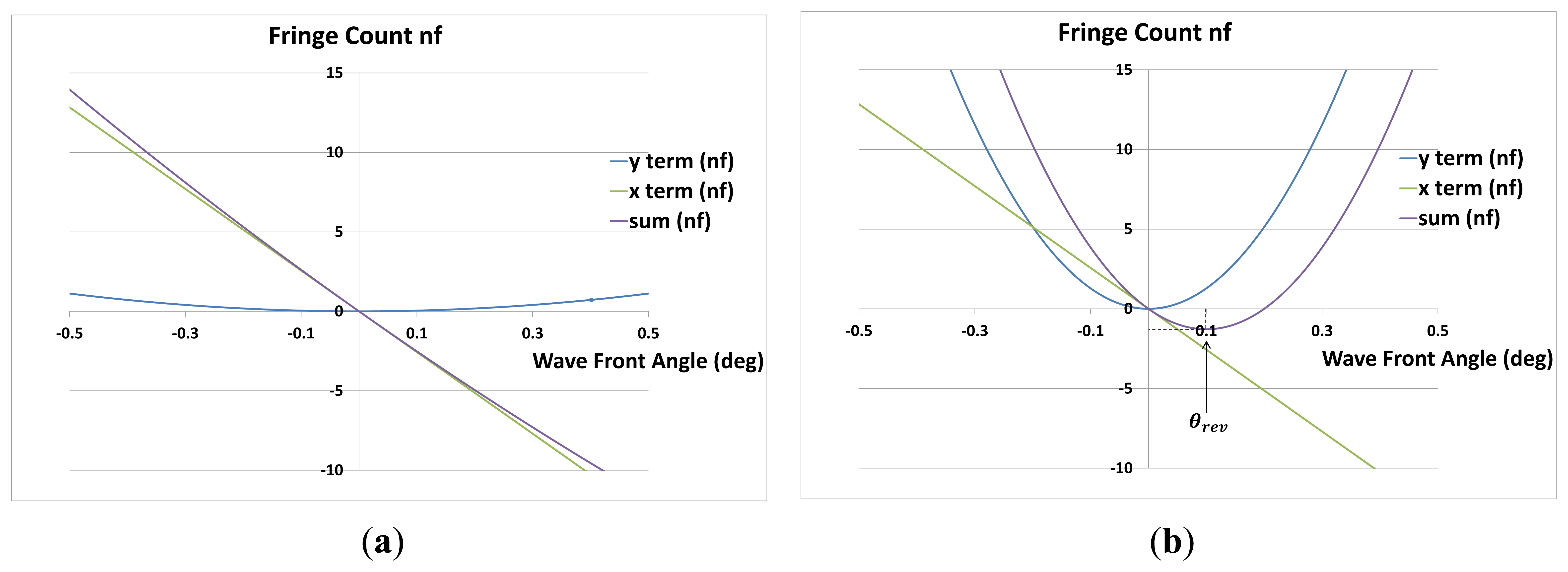
By solving Equation (28) for nf, the number of fringes lines passing over a given point (x, y) can be calculated for θ increasing or decreasing from zero to a given wave front angle:
The y term in the above equation is positive for θ ≠ 0 and is symmetrical in shape as a function of θ. For small angles sin θ = θ, therefore the coefficient of x is a linear function of angle θ. The polarity of nf, is therefore dependent on the magnitude and sign of x, θ and Δd.
nf is the number of fringes counted at a point (x, y) as θ is varied. Assume Δd = 0, there is a special case in Equation (29) when:
As discussed with Equation (28), the slope of the fringe lines is given by:
Where θ/2 is the angle of the normal of mirror M2 relative to the y-axis (Figure 2). Therefore, there is a set of points (x, y) coincident with the mirror normal that renders nf = 0.
2.5. Deriving the Speed of Fringe Movement
If Δd is considered static (Δd = 0), Equation (29) reduces to:
Taking the derivative of the x-term delivers the speed of contraction/expansion of the fringe lines at the point (x, y):
The speed of sideways deflection of the fringe lines at point (x, y) results from calculating the derivative of the y-term:
The overall fringe movement speed is therefore:
From Equation (35), the direction of fringe movement reverses if:
That is, when the perpendicular of the wave front from the origin points towards +x. The mirror tilt angle is therefore θrev/2. If y → 0, θrev → π/2, i.e., the smaller y, the larger is θrev.
From Equation (29), the fringe count returns to zero if the numerical value of x- and y-terms cancel each other out, i.e.,:
Which has solution:
This occurs at the angle θn= 0:
If x = y, then θn= 0 = π/2, if x > y, then θn= 0 > π/2 and conversely, if y > x, then θn= 0 < π/2.
The relationship between θn= 0 and θrev, results in the identity of θn= 0 ≡ 2θrev.
From Equations (37) and (40):
Resulting in:
2.6. Determination of the Damping Function of the Radiant Flux Curve
From Figure 3 it is evident that the normalised radiant flux curve oscillates about a level of 0.5 radiant flux and decreases its wave amplitude about this level with increasing wave front angle θ. As this behaviour constitutes a damped function, the radiant flux decay function is derived subsequently.
For a centred photodetector of width s and positioned at x = 0, with integral boundaries x2 = +s/2 and x1 = −s/2, y = 0 and Δd = 0, the radiant flux Φe(x1,x2) in Equation (8) reduces to:
In Equation (43), the maximal radiant flux corresponds to 2s (cf. Equations (11) and (23): radiant flux = constant * z * 2s; z is considered unity as the z-direction is perpendicular to fringe lines).
Normalising the radiant flux to 2s delivers the normalised radiant flux Φn:
As the normalised radiant flux ranges from 0 to +1, it is converted to a range from −1 to +1 in order to compare it to a standard sine function:
Equation (46) is the constitutive equation of the radiant flux decay function at x = 0 and y = 0. FD is a reciprocal function of θ, with a decay constant CD of or .
3. Results
The radiant flux and the fringe count are influenced by a range of parameters, namely the wave front angle θ, the position x of the photodetector with respect to the centre line, the laser wave length λ, the distance y between the mirror and the photodetector, and the side length s, i.e., the size of the photodetector, all of which are variable. The influence of these parameters is explained in a systematic way based on the equations derived in the Mathematical Analysis section.
3.1. Influence of θ on the Radiant Flux
The effect of θ on the magnitude of the radiant flux also depends on the values of the other abovementioned variable parameters. In order to demonstrate this, the radiant flux is examined with four different conditions, in which some parameters are kept constant whereas others are variable.
3.1.1. θ = Variable, x = 0, y = 0, s = Variable
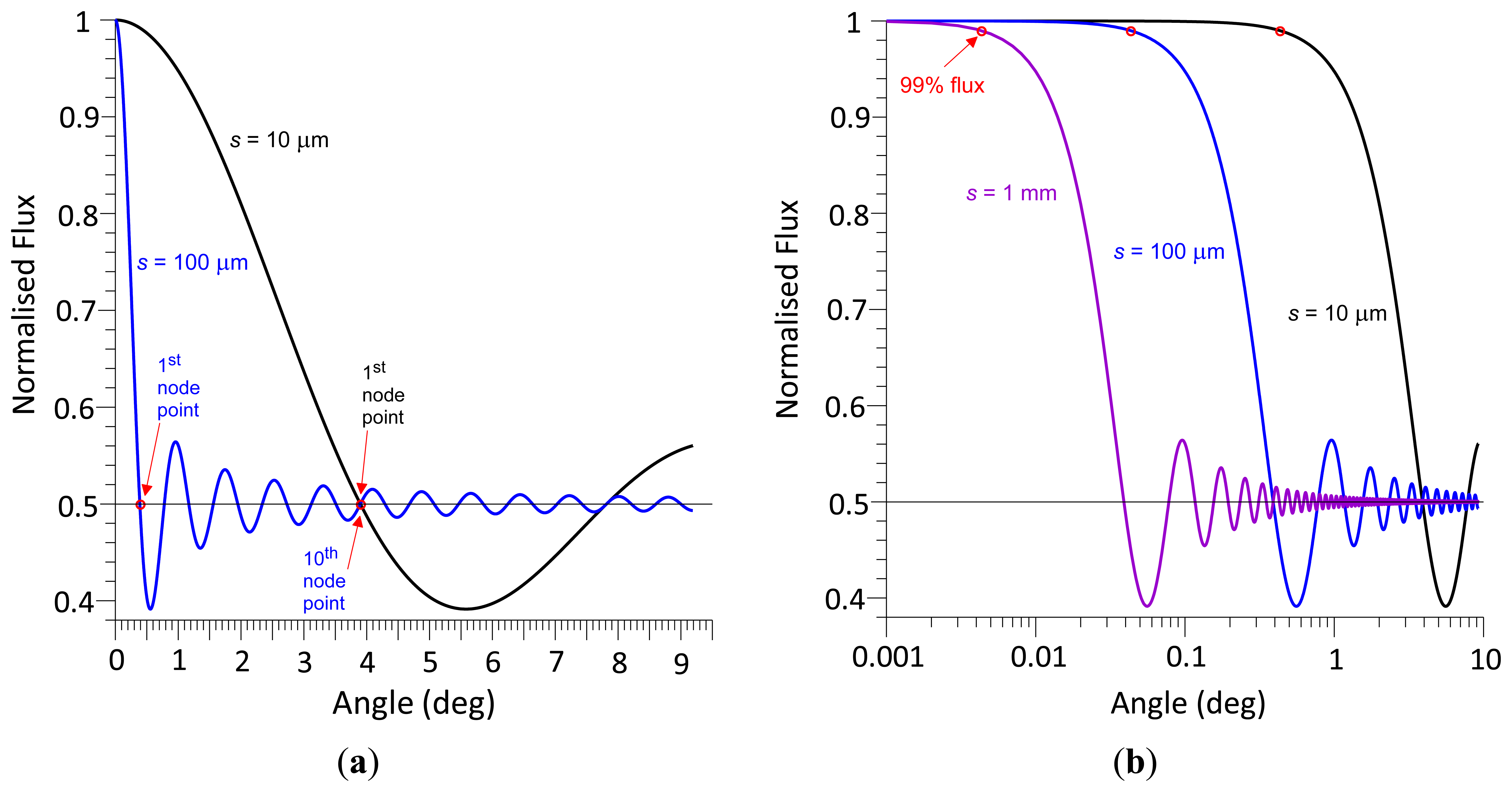
Figure 4a shows the radiant flux curves of two different photodetector areas. If θ = 0, the radiant flux is 100%. With increasing θ, the radiant flux decreases first, reaches the first primary node at a radiant flux magnitude of 50% and oscillates about the 50% level with decreasing radiant flux amplitude. The normalised radiant flux curve corresponds to a damped sine function with a damping function of 2/(skθ) or λ/(πsθ). Multiplying a sine function of the form sin (πsθ/λ), where λ/s represents the reciprocal value of the first node angle θnp, delivers a damped sine wave, which, after adding 1 and dividing the sum by 2, results in the normalised radiant flux curve. In contrast to a standard sine wave, where the first minimum is at (3/2) π, i.e., at 1.5 θnp, the non-linear decay rate causes the first minimum to be located at an angle of 1.4304 θnp, with a normalised radiant flux magnitude of 0.3913832. This magnitude is independent of s and λ.
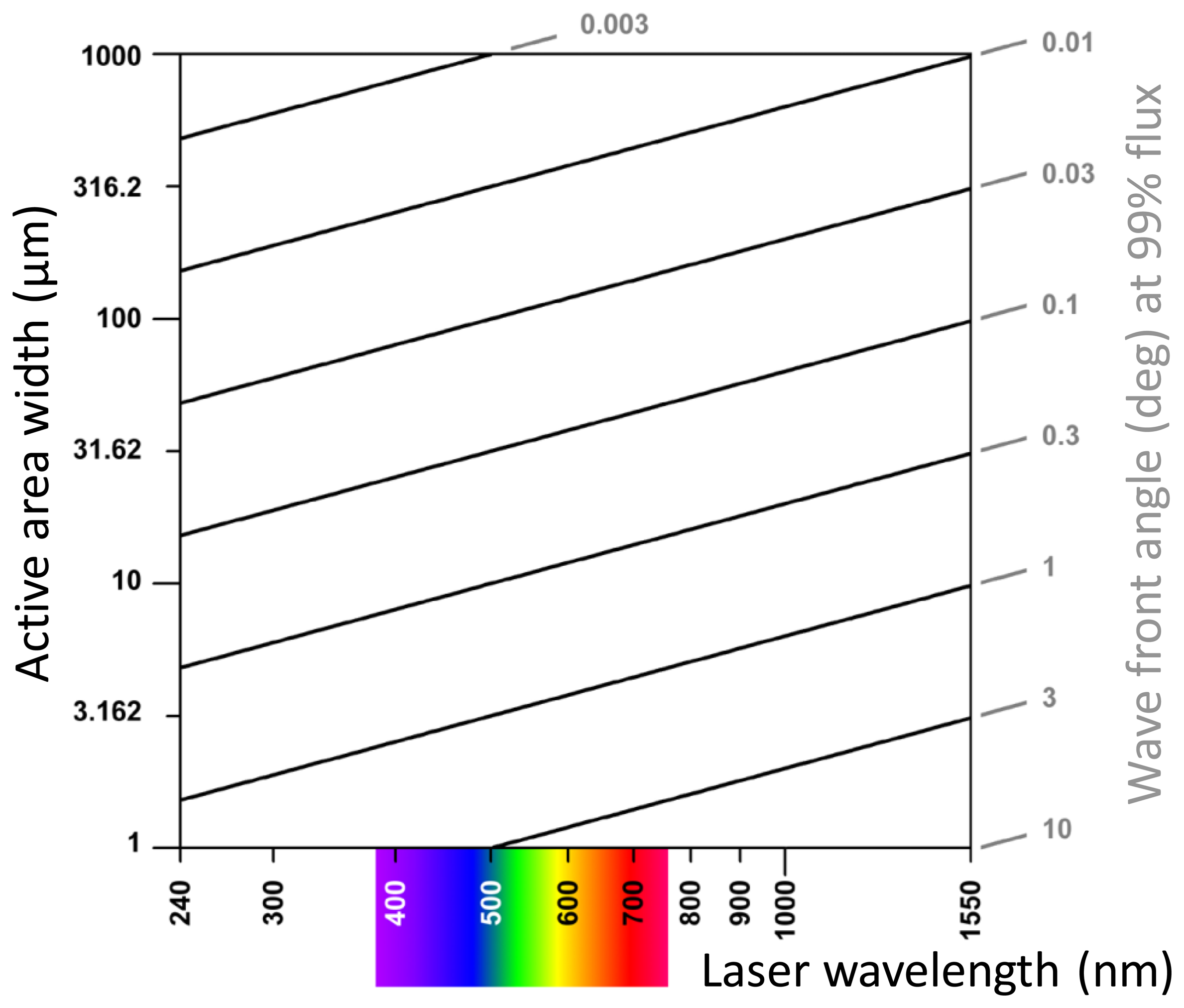
According to Equation (16), the smaller s, the larger is the wave front angle at the first node point. If s = 100 μm and λ = 680 nm, the first and tenth primary nodes are at θ = 0.3896° and 3.896°, respectively, and if s = 10 μm, the first primary node is at 3.896° (Figure 4a). The smaller is s, the slower the radiant flux decreases with increasing wave front angle. If s = 10 μm, 100 μm, and 1 mm, the angle at 99% radiant flux is located at θ = 0.43°, 0.043°, and 0.0043° (Figure 4b), respectively. According to Equation (16)s and λ have opposite effects: reducing s by a factor of two results in the same angles of primary node points and 99% radiant flux as does a two-fold increase of λ. Figure 5 exemplifies this principle in a contour plot of equal angles of 99% radiant flux as a function of s and λ.
At this point it has to be mentioned that the same radiant flux curves are obtained if y > 0 and x = y(1/sinθ – 1/tanθ) according to Equation (31). Equation (31) provides the solution for nf = 0, which deviates in x-direction if y > 0. This is explained in more detail below in the section dealing with influence on fringe count.
3.1.2. θ = Variable, x = Variable, y = 0, s = Variable
Photodetector positions x ≠ 0 changes the curves shown in Figure 4a insofar as the number of 50% radiant flux transitions is larger than the number of primary node points. The larger x, the more the radiant flux curve oscillates between the node points. In Figure 6, the radiant flux curve at x = s/2 intersects the 0.5 radiant flux level once between each pair of node points, the curve at x = s does so twice, at x = 2s four times and at x = 10s twenty times. The larger x, the higher is the density of the radiant flux curve filling up the area under the radiant flux curve at x = 0 (Figure 6b), which acts like an envelope curve for radiant flux oscillations at larger x. This is insofar important to note as it shows that the modulation amplitude of the radiant flux across x (Figure 7), is unaffected by x.
Figure 6a shows secondary node points, i.e., intersections of the two curves at radiant flux magnitudes other than 50%. Independent of the position x, all curves intersect at the primary node points. The radiant flux at the primary node points is constant (50%), whereas the radiant flux at the secondary nodes is variable and a function of x. For example, at multiples of 0.02597° (Figure 6a), the three radiant flux curves of x = s/2, s and 2s, with s = 0.001, intersect; at the 3rd and 6th intersection, the secondary nodes are identical to the primary nodes (2nd and 4th).
As the angle θ increases, so does the number of fringe lines per unit x (Figure 7). At θ = 0, the radiant flux is constant at 100%. After a slight increase in θ, the radiant flux oscillates between 100% and 0%, i.e., the maximal radiant flux is still very close to 100% (Figure 4b). Further increase in θ reduces the radiant flux amplitude, which fluctuates about 50% until the modulation amplitude converges to 0 at the 1st node point and remains constant at 50% radiant flux. Further increase in θ expands the modulation amplitude, however, the polarity of the radiant flux curve changes, i.e., peaks at x = 0 before the node point are converted to troughs after the node point.
3.1.3. θ = Variable, x = 0, y = Variable, s = Variable
When introducing the distance y between the plane of the photodetector and the tilting mirror, the radiant flux curve can be entirely below or above the 50% radiant flux level, touching it only at the primary node points (Figure 8). The radiant flux curve is then superimposed by a further oscillation of a longer wave length. At the 6th primary node point of θ = 0.23377°, the radiant flux curve does not cross the 50% radiant flux level; nevertheless, the polarity changes in the same way as shown in Figure 7. The distance y does not affect the primary node points according to Equation (16), whereas the secondary nodes are a function of y (as well as s and θ).
Increasing y (Figure 9) has the same effect as increasing x (Figure 6): the radiant flux curve oscillates more frequently under the envelope of the radiant flux at y = 0 (Figure 9a). This does not affect the modulation amplitude of the radiant flux (Figure 9b), which remains the same across x at a specific angle θ, however, the centre fringe line is more deflected off-centre with θ, the larger is y (Figure 9b).
3.1.4. θ = Variable, x = Variable, y = Variable, s = Variable
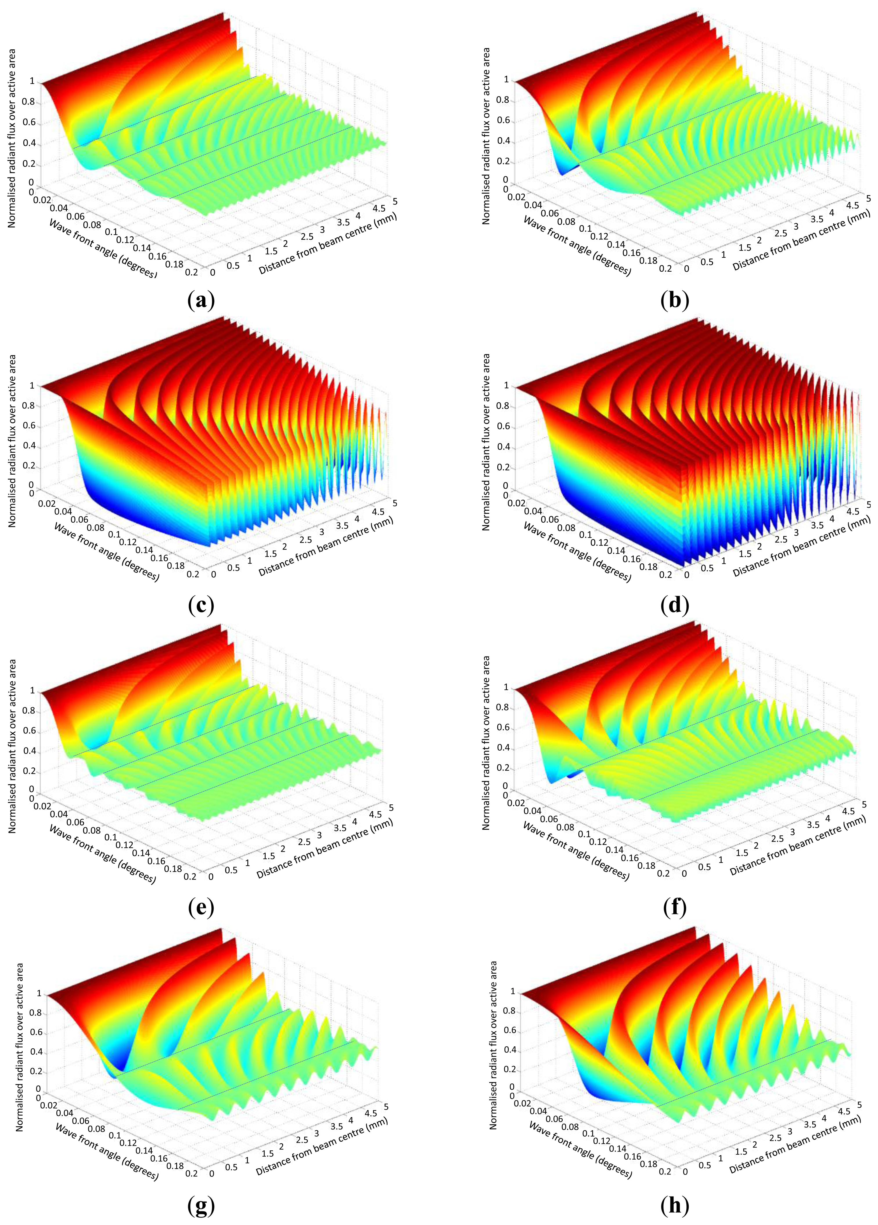
Figure 10 summarises the influence of θ, s, x, y and λ on the normalised radiant flux. The difference between Figure 10a–d is that the radiant flux before the first primary node point decays slower the smaller s is. Figure 10d shows for small angles that the modulation amplitude remains constant across x and θ.
Figure 10e,f shows with greater y, the more the centre fringe line deflects towards larger positive x and that fringe lines from the negative x-side cross over to the positive-side.
The dotted lines in Figure 10a,b,e,f shows the primary nodes for s = 1 mm, s = 0.5 mm and that the primary nodes are dependent on s and independent of y for constant λ.
Figure 10g,h shows with greater λ for equivalent s (cf.Figure 10a,b) that the interval of primary node angles is greater. Also, the radiant flux decays slower before the 1st primary node for greater λ.
Figure 10g,h shows with greater λ for equivalent s (cf. Figure 10a,b) that the radiant flux drops off slower before the 1st primary node.
Figure 10 shows at θ = 0°, the normalised radiant flux = 1 and is independent of x, s, y and λ.
3.2. Influence of x and y on the Fringe Count
The number of fringe lines nf passing over a point (x, y) within the fringe pattern is given by Equation (29), which is a function of the fringe lines tilting (y term), the fringe lines contracting/expanding (x-term) and moving mirror displacement (Δd).
Assuming Δd = 0, as the moving mirror tilts from orthogonality, fringe lines are produced with a slope that is parallel to the normal of the mirror (Equation (31) and Figure 2). The y-term in Equation (29) is linked to the slope of the fringe lines, i.e., as the wave front angle increases then so does the fringe lines (in cross-section). With x and θ static, the further the point is up the y-axis, the greater the number of fringe lines that tilt across the point. The angle θ between the two wave fronts can be positive or negative with respect to the y-axis, however, the coefficient of the y-term is always positive and therefore only has an additive effect on nf.
The x-term of Equation (29) is linked to contraction/expansion of the fringe lines with wave front angle. The focal point of the contraction/expansion is the normal of the mirror that is coincident with the axis of tilt.
With Δd = 0, as θ is increased a central fringe line is generated and aligns itself with this normal. Fringe lines develop to the left and right of this normal and contract toward it. For a given point (x, y) in the fringe pattern, as θ is increased, more and more fringe lines will develop and cross over the point. As the central fringe line is essentially static, fringe lines to the far left and right move far quicker than those closer to the central fringe line.
Figure 11 and Equation (33) confirm this behaviour showing that the speed of contraction/expansion (from the x-term of Equation (32)) of the fringe pattern is a constant. Therefore an active area located further from the centre of the beam will experience more fringe lines passing over it than one located closer to the centre when mirror M2 tilts. Parameters x and λ have opposite effects on the contraction/expansion speed.
The speed of the fringe line tilt (from the y-term of Equation (32)) results from Equation (34). This fringe tilt speed is a tangent function of the wave front angle, independent of x, i.e., of the lateral position of the photodetector, but dependent on y and λ. The speed of fringe line tilt is initially smaller than the speed of contraction, as the former is zero if θ = 0 (tan θ = 0).
Figure 12 shows the effect of increasing and then decreasing fringe numbers with progressive wave front angle. The fringe count on the positive x-side are acutely curved initially, the speed of the centre fringe line deflection lags behind the speed of contraction. Subsequently, the former speed term catches up and eventually overtakes the latter term. This results in the fringe lines initially moving over an off-centre photodetector in one direction and then moving over the same detector again but in opposite direction, thereby first increasing the fringe count and subsequently decreasing it. Figure 12 also shows that the larger x, the larger is θrev.
If Δd is dynamic and θ is variable, then the fringe count is affected by transition of the fringe lines across the photodetector due to mirror translation in addition to fringe tilt and fringe contraction/expansion. The direction of transition of the fringe lines is dependent on whether translation of the mirror is in the positive or negative y direction.
The effect of fringe tilt and y position of the photodetector can also be shown taking the photodetector parameters given in Figure 11d where s = 0.01 mm, y = 20 mm, λ = 680 nm and centering the photodetector on the y axis (i.e., x = 0 mm). From Equation (8) the normalised radiant flux is calculated to be 0.997 for a wave front angle θ of 0.05°. Relocating the photodetector at y = 100 mm returns a normalized flux of 0.938, which is reduced from the first location as a result of fringe tilt. To work out what this change in radiant flux represents in terms of change in fringe position, substitute each flux value into the equation Φ = Φ0sin(kx′), where Φ0 = 1 is the maximum flux amplitude, k = 2π/df, df = λ/θ is the fringe width and x′ represents the first and second position respectively of the fringe lines. Subtracting the two equations and solving for the change in fringe position gives 34.64 μm. Fringe width is 779.2 μm, therefore the change in fringe position due to the photodetector being located further away represents a phase difference of 16° and consequently represents a difference in nf between the two positions with varying θ.
4. Discussion
The focus of this paper has been to establish the behaviour of the radiant flux of the interferogram over a photodetector of rectangular aperture that is variable; in size; in displacement across the interferogram; and, in axial distance from the source of interference, for variable angle between the two wave fronts and variable wavelength.
The most apparent observation from the mathematical analysis in this study is that the radiant flux decays rapidly with increasing wave front angle with the recurrence of primary nodes where the radiant flux decays to 50% maximum and the modulation amplitude reduces to zero. This observation is also confirmed by [3,5–10,17] where radiant flux is calculated over a disc and also by [8,11] where the radiant flux is calculated over a square area. The modulation amplitude in this study and the literature is found to decay as a cardinal sine function. However, this study has gone further to determine that the radiant flux decays with a decay function that is a reciprocal function of the wave front angle with decay constant that is proportional to the wavelength and is inversely proportional to the photodetector active area width.
What is so far not apparent from the literature, nor is it evident in the figures, is that between each primary node the polarity of the radiant flux reverses. This phenomenon has an adverse effect on phase measurement accuracy where the wave front angle has been allowed to increase beyond a primary node and the modulation amplitude is sufficiently large enough for fringes to be counted.
In the literature [3,5–11,17], the boundary of the radiant flux calculation is centred on the interferogram, giving just a single radiant flux curve decaying as a cardinal sine function. Whereas, in this study, the radiant flux boundary is derived to be variable across the interferogram. This variant shows that as the boundary is moved off centre, the radiant flux oscillates increasingly about the 50% normalised maximum as an integer multiple of the distance from centre. Additionally, the amplitude of the oscillation is bounded by the centred radiant flux curve.
A further finding from this study, which to the best of our knowledge, is not mentioned in the literature is how the radiant flux is affected when the fringe lines tilt and contract/expand with varying wave front angle. Having included as an integral parameter the axial distance of the photodetector from the interferometer, it is found for a centred photodetector that fringe tilt initially lags fringe contraction, but then fringe tilt becomes increasingly dominant on the radiant flux with increasing distance of the photodetector from the beamsplitter.
Interferometry applications that use a plane flat mirror with translation stage, and discrete photodetectors [12–15] or position sensitive device [16] will suffer erroneous measurements if the wave front angle is not limited to give acceptable modulation amplitude. This can be done by choosing an appropriate photodetector aperture width that is an order of magnitude less than the fringe line spacing. Increasing the wavelength improves modulation amplitude for equivalent photodetector aperture widths.
If the wave front angle varies beyond primary node angles the radiant flux reverses polarity introducing an additional error with a π radian phase change in photodetector output.
Alignment of the photodetector with the centre of the interferogram reduces the susceptibility of the fringe lines crossing over the photodetector as they contract as a linear function of distance from centre with increasing wave front angle.
Finally, the tilt angle of the fringe lines increases with increasing wave front angle and they cross over the central axis of the interference beam with increasing distance from the beamsplitter. Therefore to limit the error in measurement that this produces, the photodetector should be located as close as possible to the beamsplitter.
5. Conclusions
The radiant flux Φ across the active area of a photodetector is a damped sine function (i.e., a cardinal sine function) of the wave front angle θ, with a reciprocal decay of the ratio of wavelength λ to detector width s. The larger s and the smaller λ, the faster is the decay of the radiant flux.
If the radiant flux magnitude at wavefront angle θ = 0 is normalised to 100%, then the radiant flux magnitude at the primary node points is 50% and at the first minimum is 39.14%. The polarity of the radiant flux changes exclusively at every primary node point. The radiant flux magnitude at specific θ is independent of any parameter if the centre of the fringe beam coincides with the centre of the photodetector.
The larger the distance x of the photodetector from the centre of the fringe beam and/or the distance y between mirror and photodetector, the more the radiant flux oscillates under the envelope radiant flux curve generated if x and y = 0. These two parameters do not affect the modulation amplitude of the radiant flux.
The movement of fringe lines with increasing θ is a combined effect of fringe contraction (x-dependent; the faster the more the detector is off centre) and fringe tilt (y-dependent; the faster the larger y). Fringe contraction and tilt movement can have opposite effects, with fringe contraction lagging behind fringe tilt, such that the fringe count first increases, then decreases and then returns to zero.
Consequently, significant fringe count errors occur if the photodetector is operated near or beyond primary nodes where radiant flux modulation reduces to zero and then changes polarity, or if the x and y distances of the photodetector are large therefore increasing the fringe contraction and fringe tilt influence.
Acknowledgments
The authors thank Christophe Fumeaux for invaluable comments on the manuscript.
Appendix
This appendix provides a detailed derivation of the equations in the paper “Theoretical Analysis of Interferometer Wave Front Tilt and Fringe Radiant Flux on a Rectangular Photodetector” by authors R.M. Smith and F.K. Fuss.
The equation numbers in this appendix follows the equation numbering in the parent paper, however, where additional equations are included they are designated an alphanumeric reference.
A1. Derivation of the Equation for Radiant Flux
The electric field of a plane wave is given by Equation (A1)
where E is the time (t) dependent electric field, r is the unit vector of the electric field in 3 dimensional space, i.e., r = xx̂ + yŷ + zẑ and x̂, ŷ and ẑ are unit vectors along the x, y and z axes, E0 is the vector amplitude of the wave, k is the wave vector where k = ku, where u is the unit vector defining the direction of propagation and , λ is the wavelength of the light source, k is the wave number and ω is the angular frequency of the wave.
Figure 2 depicts the linear optical equivalent of the Michelson interferometer with the virtual source wave front approaching mirrors M1 and M2 from the top of the figure. With reference to the origin, the reflected wave fronts 1 and 2 from respective mirrors have wave vectors k1 and k2.
Also depicted in Figure 2, the source wave front travels a distance Δd further to M1 before it is reflected. Therefore, the optical path difference (OPD) between wave fronts 1 and 2 is 2Δd resulting in wave front 1 having a phase lag of k2Δd relative to wave front 2.
The sum of the electric fields of wave fronts 1 and 2 is therefore
The irradiance I of an electric field is given by Equation (A6) and is the radiant flux of the electric field delivered per area to a given surface with units Wm−2. i.e., radiant flux density
Where nRI is the refractive index of the medium, c is the speed of light in vacuum, ε0 is the vacuum permittivity, and the complex conjugate of Esum.
Equation (A7) indicates that the irradiance at a point (x, y) in the fringe pattern created by wave fronts 1 and 2 is dependent on the values of x and y, wave number k, which is a function of wavelength, the angle θ between the wave fronts and the optical path difference 2Δd.
If Equation (A7) is integrated along the x-axis between arbitrary points x1 and x2 and then multiplied by side length z in the z -direction to create an area across the photodetector, the solution is the radiant flux incident on a rectangle of side lengths x2 –x1 = s and z. As mirror M2 is only tilted about the z-axis, variable z does not need to be included in the integration as it behaves purely as a multiplier to the solution of the integration along the x-axis. Therefore:
The radiant flux Φe given by Equation (A8) is expressed in Watts (W) and is the total radiant power of the interference beam incident on the defined rectangular active area of the photodetector. At θ = 0, which is indeterminate, therefore applying L'Hôpital's rule to the integral solution of Equation (A8) for θ → 0 returns:
Therefore, as θ → 0, the radiant flux derived in Equation (A8) tends to
It is worth noting that at θ = 0, the irradiance in Equation (A7) reduces to
Equation (A10) indicates that as θ → 0 the magnitude of the radiant flux is dependent on the area z · s, k and Δd but is independent of y.
The irradiance and radiant flux in Equations (A10) and (A10a) are maximum when cos(k2Δd) = 1, i.e., when 2Δd = nfλ, where nf is an integer equivalent to the number of fringe lines and 2Δd is the optical path difference. Whenever the OPD is an integer multiple of the wavelength, the two wave fronts in Figure 2 are in phase with one another resulting in maximum radiant flux, i.e.,
To demonstrate the behaviour of the radiant flux over differing integral boundaries, Figure 3 shows the radiant flux curves for two sets of integral boundaries that are equal in length with assigned variables defined as follows that have been substituted in Equation (A10); y = 0 m, λ = 680 × 10−9 m therefore k = 9239978, Δd = 0 m, integral width s = 0.001m, red curve integral boundaries x2 = 0.0005 m, x1 = −0.0005 m, blue curve integral boundaries x2 = 0.001 m, x1 = 0 m.
It can be seen from the Figure 3 what appears to be node points at half the normalised radiant flux that are cyclic, which have been termed primary nodes, and this phenomenon is explored further below. What is also noticeable is the two curves converge as θ → 0 as predicted in Equation (A10).
A2. Identifying Specific Wave Front Angles θn With Invariable Φe for Two Sets of Integral Boundaries
To analyse the effect of mirror tilt angle on two separate rectangular areas of equal size and determine the node points observed in Figure A1, consider only the integral solution of Equation (A8). If we define the two intervals along the x-axis with upper and lower limits x1, x2 & x3,x4 such that x2 – x1 = x4 – x3 = s and substitute in the Equation (A8) we get after simplification Equations (A12) and (A13):
To solve for θ and x, let Equation (A12) = Equation (A13)
Applying the identity below and simplifying Equation (A13b) yields Equation (A14).
To obtain the node points that satisfy Equation (A14) for the two intervals defined above, i.e., x2 – x1 = x4 – x3 = s, values need to be assigned to these boundary limits. For example, let x1, x2 & x3, x4 be the two intervals depicted along the plane of the photodetector in Figure A1 with values defined as x1 = − s; x2 = 0; x3 = − s /2; x4s/2.
Substituting these values in Equation (A14) and simplifying yields:
The equality of Equation (A15) is satisfied if
and/ or
Solving:
- (a)
is satisfied when , where np is an integer related to what are termed primary nodes (see Figure 3), resulting in:
if small angles are considered, implying sin θnp = θnp, where the intersection of the two radiant flux curves at θnp is called a primary node and θnp is called the primary node angle.- (b)
is satisfied when
There are two solutions that satisfy Equation (A17):
- (i).
(− s) sin θ = 0, therefore sin θ0 = 0 where θ0 = 0. As only small angles are of concern, θ = nπ is irrelevant. Note that θ0 = 0 is co-incident with primary node np = 0 from Equation (A16)
- (ii).
The cosines are identical for , where δ is a phase shift and ns is an integer related to secondary nodes, i.e.,
ns can be zero if the data is mirrored about θ = 0 and ns = 1 if the data is mirrored about θ = π.
From Equations (A17) and (A18) there are 2 identities:
As the left- and right-hand terms refer to the same angle θ
Therefore:
The 2nsπ term in Equations (A18e) and (A18f) lies exactly between
Therefore:
This eliminates the unknown term Δ and provides the function for secondary nodes. Simplifying Equation (A18k) renders:
Rearranging and grouping terms yields:
Let
By way of demonstrating the presence of secondary nodes for the case with integral boundaries defined above as x1 = − s/2; x2 = 0; x3 = − s/2; x4 = s/2, firstly, assume Δd = 0 m.
Equations (A18s), (A18t) and (A18u) now reduce to:
Then, the variables in Equations (A18x)–(A18z) are assigned values, for example those defined in Equation (A18A).
Finally, Equation (A18w) is solved for different ns (positive and negative) to find θns where the radiant flux curves intersect at the secondary node points.
Secondary nodes for the above defined conditions are returned for
Also
Consider the solution defined by Equation (A18B) and let ns = − 1. The secondary node point is calculated by this solution, i.e., θ−1 = 0.07409° and confirmed by substituting the above conditions into the integral part of Equation (A8).
Mirror M2 in Figure A1 can tilt left or right of the y-axis, therefore θns can be positive or negative, therefore returning secondary nodes of both polarities for θns in Equations (A18B) and (A18C).
From the above derivation of the secondary nodes, a specific solution was obtained for the defined intervals specified in as x1 = − s; x2 = 0; x3 = − s/2; x4 = s/2 and the variable values assigned in Equation (A18A). The occurrence of secondary nodes is unique and specific to the defined integral boundaries x1, x2 & x3, x4, the values of k, y and Δd. Consequently, the cosine expression in Equation (A14) has to be solved accordingly with its own set of boundary conditions, such as Equation (A18A). The wave front angle at secondary node angles θns is incidental, unlike at primary nodes, which is cyclic and dependent only on k and s (sine expression in Equation (A14)). The next section derives the magnitude of the radiant flux at the primary nodes.
A3. Determination of the Magnitude of Φe at Wave Front Angles θn
To determine the magnitude of the radiant flux of the fringe pattern at the primary nodes we solve Equations (A12) and (A13) independently for the intervals defined as x1 = − s; x2 = 0; x3 = − s/2; x4 = s/2. Beginning with Equation (A12):
For small angles sin θ = θ, therefore Equation (A19) becomes
At θ0, Equation (A20) reduces to 0/0, which is indeterminate. Therefore applying L'Hôpital's rule:
Repeating the above for Equation (A13)
For small angles sin θ = θ, therefore Equation (A21a) becomes
At θ0, Equation (A20) reduces to , which again is indeterminate. Applying L'Hôpital's rule
Equations (A21) and (A21c) show that as θ → 0 the radiant flux becomes equal for the integral boundaries defined as x1 = − s; x2 = 0; x3 = − s/2; x4 = s/2. Substituting the result of Equation (A21) or Equation (A21c) into Equation (A8) gives Equation (A22), which shows the magnitude of the radiant flux as θ→0 is dependent on k and Δd and independent of y.
Note Equations (A10) and (A22) are equal, resulting in maximum radiant flux for translations where 2Δd = nλ.
To work out the value of radiant flux for all other values of θnp, i.e., θ1, 2, 3,.., substitute inline from Equation (A16) into Equation (A20) and Equation (A21b) independently. Beginning with Equation (A20) and using the identity in Equation (A13b):
Repeating the above for Equation (A21b)
Equations (A23a) and (A24) give the same result for the integral of the active areas at θnp = θ1,2,3,.. and therefore the radiant flux at these wave front angles is given by Equation (A25).
Equation (A25) also shows that the radiant flux at θnp = θ1,2,3,.. is half maximum (cf. Equation (A23)), and in contrast to the radiant flux at θnp = θ0 given in Equation (A22), Φe(θ1,2,3,..) is independent of k and Δd. The reason for this is the width s of the active area is an integer multiple of the fringe line spacing at primary node angles θnp = θ1,2,3,…
When there is an exact multiple of fringe lines within the active area, the radiant flux across the active area is the mean of the maximum constructive and destructive interferences, i.e., 50 %. This means that if the active area is moved in either direction along the x-axis, the radiant flux remains static at 0.5 normalised magnitude. If mirror M2 translates, there will be no change in the radiant flux despite the fringe pattern moving back and forth across the active area.
A4. Effect of Distance x and y of Photodetector from Origin with Varying θ
To determine the effect of distance y of the photodetector from the origin with varying θ, the position and slope of the fringe lines needs to be determined. This is done by finding the instances of maximum value of irradiance in Equation (A7), i.e., when
Equation (A26) is true when
Equation (A28) is a linear equation and defines the profile of the fringe pattern in the x-y plane as illustrated in Figure A1 where is the slope of the fringe lines and is the y intercept. As only small angles are being considered it becomes indeterminate at θ = 0, which stands to reason as the fringe pattern is uniform across the active area as well as the x-y plane and no fringe lines are present.
By solving Equation (A28) for nf, the number of fringes lines passing over a given point (x,y) can be calculated for θ increasing or decreasing from zero to a given wave front angle.
The y term in the above equation is positive for θ ≠ 0 and is symmetrical in shape as a function of θ.
For small angles sin θ = θ, therefore the coefficient of x is a linear function of angle θ.
The polarity of nf is therefore dependent on the magnitude and sign of x, θ and Δd.
When θ= 0, Equation (A29) reduces to
As discussed with Equation (A28), the slope of the fringe lines is given by:
Deriving the speed of fringe movement
If Δd is considered static (Δd = 0), Equation (A29) reduces to
Taking the derivative of the x-term delivers the speed of concertinaing of the fringe lines at the point (x, y).
The speed of sideways deflection of the fringe lines at point (x, y) results from calculating the derivative of the y-term
The overall fringe movement speed is therefore
From Equation (A35), the direction of fringe movement reverses if
And therefore the angle of movement reversal θrev is
That is, when the perpendicular of the wave front from the origin points towards +x. The mirror tilt angle is therefore θrev/2. If y → 0, θrev → π/2, i.e., the smaller y, the larger is θrev.
From Equation (A29), the fringe count returns to zero if the numerical value of x- and y-terms cancel each other out.
This occurs at the angle θn= 0
If x = y, then , if x > y, then and conversely, if y > x, then .
The relationship between θn= 0 and θrev, results in the identity θn= 0 ≡ 2θrev.
From Equations (A37) and (A40)
Resulting in
And proving the identity of θn= 0 ≡ 2θrev being correct.
Determination of the damping function of the flux curve
From Figure 4 it is evident that the normalised flux curve oscillates about a level of 0.5 flux and decreases its wave amplitude about this level with increasing wave front angle θ. As this behaviour constitutes a damped function, the flux decay function is derived subsequently.
For a centred photodetector of width s and positioned at x = 0, with integral boundaries & , y = 0 and Δd = 0, the radiant flux Φe(x1,x2) in Equation (A8) reduces to
In Equation (A43), the maximal flux corresponds to 2s (cf. Equations (A11) and (A23): flux = constant * z * 2s; z is considered unity as the z-direction is perpendicular to fringe lines).
Normalising the flux to 2s delivers the normalised flux Φn
As the normalised flux ranges from 0 to +1, it is converted to a range from −1 to +1 in order to compare it to a standard sine function
For small θ, Equation (A45) becomes
This equation defines a damped sine function. The equivalent undamped sine function has the form of
Where A is the amplitude and f is the reciprocal value of 2nd node angle ( ), i.e., the wave length of the flux function. Substituting this term into Equation (A45b) yields
The decay function FD is obtained when normalising the damped sine function to its undamped counterpart
After simplifying and considering that θ is small
Considering that
Equation (A46) is the constitutive equation of the flux decay function at x = 0 and y = 0. FD is a reciprocal function of θ, with a decay constant CD of or .
Conflicts of Interest
The authors declare no conflict of interest.
References
- Michelson, A.A. The relative motion of the earth and the luminiferous ether. Am. J. Sci. 1881, 22, 120–129. [Google Scholar]
- Michelson, A.A.; Morley, E.W. On the relative motion of the earth and the luminiferous ether. Am. J. Sci. 1887, 34, 333–345. [Google Scholar]
- Stroke, G.W. Photoelectric fringe signal information and range in interferometers with moving mirrors. J. Opt. Soc. Am. 1957, 47, 1097–1103. [Google Scholar]
- Connes, J. Recherches sur la Spectroscopie par Transformation de Fourier. Rev. Opt. 1961, 40. [Google Scholar]
- Cohen, D.L. Performance degradation of a Michelson interferometer when its misalignment angle is a rapidly varying, random time series. Appl. Opt. 1997, 36, 4034–4042. [Google Scholar]
- Välikylä, T.; Kauppinen, J. Modulation depth of Michelson interferometer with Gaussian beam. Appl. Opt. 2011, 50, 6671–6677. [Google Scholar]
- Kunz, L.W.; Goorvitch, D. Combined effect of a converging beam of light and mirror misalignment in Michelson interferometry. Appl. Opt. 1974, 13, 1077–1079. [Google Scholar]
- Peck, E.R. Integrated flux from a Michelson or corner-cube interferometer. J. Opt. Soc. Am. 1955, 45, 931–934. [Google Scholar]
- Murty, M.V.R.K. Some more aspects of the Michelson interferometer with corner cubes. J. Opt. Soc. Am. 1960, 50, 7–10. [Google Scholar]
- Williams, C.S. Mirror misalignment in Fourier spectroscopy using a Michelson interferometer with circular aperture. Appl. Opt. 1966, 5, 1084–1085. [Google Scholar]
- Yang, Q.; Zhou, R.; Zhao, B. Principle of the moving-mirror pair interferometer and tilt tolerance of the double moving mirror. Appl. Opt. 2008, 47, 2486–2493. [Google Scholar]
- Chang, C-W.; Hsu, I-J. Composite low-coherence interferometer for imaging of immersed tissue with high accuracy. P. Soc. Photo Opt. Ins. 2012, 8493. [Google Scholar] [CrossRef]
- Ho, H.P.; Lo, K.C.; Hung, Y.Y. Quantitative phase modulation from a free-running Michelson Interferometer by using a novel quadrature Moiré grating with misalignment compensation. Opt. Eng. 2006, 45. [Google Scholar] [CrossRef]
- Li, R.-J.; Fan, K.-C.; Huang, Q.-X.; Qian, J.-Z.; Gong, W.; Wang, Z.-W. Design of a large-scanning contact probe for nano-coordinate measurement machines. Opt. Eng. 2012, 51. [Google Scholar] [CrossRef]
- Kim, J.W.; Kang, C.-S.; Kim, J.-A.; Cho, M.; Kong, H.J. A compact system for simultaneous measurement of linear and angular displacements of nano-stages. Opt. Exp. 2007, 15, 15759–15766. [Google Scholar]
- Prévost, C.; Genest, J. Dynamic alignment of a Michelson interferometer using a position sensitive device. P. Soc. Photo Opt. Ins. 2004, 5528, 293–304. [Google Scholar]
- Genest, J.; Tremblay, P.; Villenaire, A. Throughput of tilted interferometers. Appl. Opt. 1998, 37, 4819–4822. [Google Scholar]
- Peña-Arellano, F.E.; Speake, C.C. Mirror tilt immunity interferometer with a cat's eye retroreflector. Appl. Opt. 2011, 50, 981–991. [Google Scholar]
- Maxwell, J.C. A dynamical theory of the electromagnetic field. Philos. T. Roy. Soc. A. 1865, 155, 497–501. [Google Scholar]
- Peatross, J.; Ware, M. Physics of Light and Optics; Brigham Young University: Provo, UT, USA, 2011. [Google Scholar]


© 2013 by the authors; licensee MDPI, Basel, Switzerland. This article is an open access article distributed under the terms and conditions of the Creative Commons Attribution license (http://creativecommons.org/licenses/by/3.0/).
Share and Cite
Smith, R.; Fuss, F.K. Theoretical Analysis of Interferometer Wave Front Tilt and Fringe Radiant Flux on a Rectangular Photodetector. Sensors 2013, 13, 11861-11898. https://doi.org/10.3390/s130911861
Smith R, Fuss FK. Theoretical Analysis of Interferometer Wave Front Tilt and Fringe Radiant Flux on a Rectangular Photodetector. Sensors. 2013; 13(9):11861-11898. https://doi.org/10.3390/s130911861
Chicago/Turabian StyleSmith, Robert, and Franz Konstantin Fuss. 2013. "Theoretical Analysis of Interferometer Wave Front Tilt and Fringe Radiant Flux on a Rectangular Photodetector" Sensors 13, no. 9: 11861-11898. https://doi.org/10.3390/s130911861