Analytic Performance Prediction of Track-to-Track Association with Biased Data in Multi-Sensor Multi-Target Tracking Scenarios

Abstract

An analytic method for predicting the performance of track-to-track association (TTTA) with biased data in multi-sensor multi-target tracking scenarios is proposed in this paper. The proposed method extends the existing results of the bias-free situation by accounting for the impact of sensor biases. Since little insight of the intrinsic relationship between scenario parameters and the performance of TTTA can be obtained by numerical simulations, the proposed analytic approach is a potential substitute for the costly Monte Carlo simulation method. Analytic expressions are developed for the global nearest neighbor (GNN) association algorithm in terms of correct association probability. The translational biases of sensors are incorporated in the expressions, which provide good insight into how the TTTA performance is affected by sensor biases, as well as other scenario parameters, including the target spatial density, the extraneous track density and the average association uncertainty error. To show the validity of the analytic predictions, we compare them with the simulation results, and the analytic predictions agree reasonably well with the simulations in a large range of normally anticipated scenario parameters.

1. Introduction

In distributed multi-sensor surveillance systems, the process of associating sets of local estimates from multiple sensors is a fundamental problem, named track-to-track association (TTTA) [1,2]. It is valuable for predicting the performance of TTTA, not only in multi-sensor tracking system design, but also in subsequent situation assessment and on-line resource allocation, such as sensor tasking. Generally, performance evaluation mainly depends on Monte Carlo simulations, which are expensive and time-consuming. Furthermore, little insight can be obtained for the intrinsic relationship between the relevant scenario parameters and the performance based on numerical simulations. Therefore, analytic prediction of data association performance, which does not resort to detailed and costly simulations, is of significant practical and theoretical importance.

With respect to the analytic performance prediction of data association, Sea and Singer did pioneering work on the performance analysis of the nearest neighbor (NN) algorithm [3,4]. Saha provided a methodology for predicting the performance of a logic based ESM/radar TTTA algorithm [5]. Li et al. introduced the hybrid conditional averaging technique to predict the performance of the NN tracker [6]. Mei et al. gave the formula to calculate the theoretical probability of false association for TTTA using multiscan data [7]. Mori et al. derived an analytic expression, named the exponential law, to predict the performance of the global nearest neighbor (GNN) algorithm in terms of the probability of correct association [8,9]. On the basis of Mori's work [8], Ruan et al. developed an analytic performance prediction method for the feature-aided GNN algorithm [10]. Some oversimplified assumptions were employed in the derivations, including no false alarm, perfect detection, identical diagonal elements and all other identical elements in the feature confusion matrix, etc. Areta et al. presented procedures to calculate the probability that the measurement or the track originating from an extraneous target misassociated with a target of interest for the cases of NN and GNN association [11,12]. Mori et al. quantified the utility of additional feature/attribute information for TTTA in [13]. Although these works exhibit various degrees of success, they all do not take the impact of sensor biases on TTTA into consideration.

In performing multi-target tracking with a sensor network, the systematic errors, i.e., sensor biases, can hinder the fusion of data from multiple sensors. Specifically, TTTA is always problematic with biased data, while sensor bias registration usually requires correctly associated data. That is, association and registration actually affect each other [14,15]. To fix this problem, many approaches were proposed to formulate association and registration as a joint optimization problem. However, these joint problems are very difficult to solve, due to the combinatorial nature of the problem and the non-convexity of the objective function [14–19]. Suboptimal solutions are obtained by performing association and registration in an alternately iterative manner. To a certain degree, the prediction of TTTA performance with biased data is also helpful for designing these joint association and registration algorithms.

A number of TTTA algorithms are built upon the GNN criterion [1,2,16,20–23]. Most of them can be decomposed into two steps. The first step is to construct a matrix of association costs (or negative log-likelihood) between two sets of tracks. The second step usually consists of running a linear assignment algorithm on this cost matrix to determine the maximum likelihood association by globally minimizing the cost. The construction of the cost matrix was well discussed in [22–24]. For the second step, many optimal linear assignment algorithms, such as Munkres [25], Jonker-Volgenant [26] and Jonker-Volgenant-Canstenon [27], can be adopted to identify the optimal associations. In this paper, we pay particular attention to predicting the performance of the GNN association algorithm with biased data analytically It should be noted that Castella [28] did consider the influence of biases on the performance of the multiple site track correlation technique proposed by Singer and Kanyuck [29], but the TTTA method of Singer and Kanyuck applies a gating technique and makes the association decision based on the NN rule, rather than the GNN criterion. The goal of our study is to extend the results in [8,9], which established an effective approach for predicting the performance of the optimal assignment algorithms, in an attempt to incorporate the impact of sensor biases.

The rest of the paper is structured as follows. Section 2 describes the single-scan TTTA problem. Section 3 presents the existing analytic prediction results of the bias-free situation. Section 4 provides the analytic prediction results for the GNN association algorithm with biased data. These results are verified via simulations in Section 5. Section 6 concludes the paper.

2. Problem Statement

In this paper, we consider a two-sensor single-scan TTTA problem. Although TTTA using multi-scan data has been theoretically proven to be better than that using single-scan data in [7], the former has higher computational complexity and may, in practice, exhibit lower power. That is because using multiscan data increases the degree of freedom of the test statistics, which has a negative impact on the power of the test [30,31]. Therefore, we focus on the single-scan TTTA problem, which is a data association problem with two random point sets in an m-dimensional Euclidean space, ^m.

At a given time (without the time argument, for simplicity), the track set available at sensor A is denoted by ${\left({\mathbf{\text{y}}}_i,{\mathbf{\text{P}}}_A^i\right)}_{i=1}^{N_A}$, where y_i ∈ ^m and ${\mathbf{\text{P}}}_A^i\in {\mathcal{R}}^{m\times m}$ are the state estimate and error covariance matrix of the i-th target at sensor A, respectively; N_a represents the number of tracks available at sensor A. Similarly to sensor A, the track set made by sensor B is ${\left({\mathbf{\text{z}}}_j,{\mathbf{\text{P}}}_B^j\right)}_{j=1}^{N_B}$ where z_j ∈ ^m and ${\mathbf{\text{P}}}_B^j\in {\mathcal{\text{R}}}^{m\times m}$ are the state estimate and error covariance matrix of the j-th target at sensor B, respectively; N_b represents the number of tracks available at sensor B. Let y₀ and z₀ represent the dummy tracks of sensor A and B, respectively. When a track in a list is not associated with any track from the other list, it will be assigned to the dummy track. Following [8,32], we can define the association between the two track sets as a one-to-one mapping, a. Its domain is Dom(a) ⊆ $ℐ$ = {1,…, N_A}, and its range is Rng(a) ⊆ = {1, …, N_B}. For i ∈ Dom(a), a(i) is the index of the track from sensor B associated with track i from sensor A. Tracks in $ℐ$ \ Dom(a) are associated with z₀, while tracks in \ Range(a) are assigned to y₀.

Let a* be the ground-truth association mapping. The track model is given as follows. We assume that sensors have translational biases on their local estimates of targets. The biases are modeled as additive constants. For a common target, i, we have:

$${\mathbf{\text{y}}}_i={\mathbf{\text{x}}}_i+{\mathbf{\text{b}}}_A+{\mathbf{\text{u}}}_i,$$

(1)

$${\mathbf{z}}_{a^{*}(i)}={\mathbf{x}}_i+{\mathbf{b}}_B+{\mathbf{v}}_i,$$

(2)

where x_i is the real state of target i, b_A, b_B represent the biases of sensor A and B, respectively, u_i, v_i are the random state estimation errors of target i at sensor A and B, respectively, and ${\mathbf{\text{u}}}_i~\mathcal{N}\left(0,{\text{P}}_A^i\right)$, ${\mathbf{\text{v}}}_i~\mathcal{N}\left(0,{\text{P}}_B^i\right)$.

The association can also be defined as an (N_A + 1) ×(N_B + 1) matrix h between ${\left({\mathbf{\text{y}}}_i\right)}_{i=0}^{N_A}$ and ${\left({\mathbf{\text{z}}}_{\text{j}}\right)}_{j=0}^{N_B}$, with (i, j) element h_ij for i = 1, …, N_A + 1, j = 1, …, N_B + 1, such that

$$h_{\mathit{\text{ij}}}=\{\begin{array}{ll}1,\hfill & \mathit{\text{if}}{\mathbf{\text{y}}}_i,{\mathbf{\text{z}}}_j\mathit{\text{are from the same target}}\hfill \\ 0,\hfill & \mathit{\text{otherwise}}\hfill \end{array}.$$

(3)

The relationship between a and h is: if a(i) = j, then h_ij = 1; if i ∈ $ℐ$ \ Dom(a), then h_i,0 = 1; if j ∈ \ Range(a), then h_0,j = 1; otherwise h_i,j = 0.

The GNN algorithm determines the best association decision from all possibilities by minimizing the overall cost [1,2]:

$$\underset{\mathbf{\text{h}}}{min}\sum _{i=0}^{N_A}\sum _{j=0}^{N_B}{D}_{ij}{h}_{ij}$$

(4)

subject to the constraints:

$$\sum _{i=0}^{N_A}{h}_{\mathit{\text{ij}}}=1,j\ne 0$$

(5)

$$\sum _{j=0}^{N_B}{h}_{\mathit{\text{ij}}}=1,i\ne 0$$

(6)

$$h_{\mathit{\text{ij}}}\in \{0,1\}.$$

(7)

Constraints (5) and (6) guarantee that each track from a list is assigned to one and at most one track from the other list or to the dummy track. In problem (4), D_ij (i, j ≠ 0) is the cost between y_i and z_j, defined by their normalized distance as:

$$D_{\mathit{\text{ij}}}={\Vert {\mathbf{\text{z}}}_j-{\mathbf{\text{y}}}_i\Vert }_{{\mathbf{\text{S}}}_{i,j}^{-1}}^2,$$

(8)

where ‖x‖_M denotes a semi-norm of a vector, x, defined by a nonnegative symmetric matrix, M, as ${\Vert \mathbf{\text{x}}\Vert }_{\mathbf{\text{M}}}=\sqrt{{\mathbf{\text{x}}}^T\mathbf{\text{Mx}}}$; S_i,j is the average association uncertainty covariance matrix and ${\mathbf{\text{S}}}_{i,j}={\mathbf{\text{P}}}_A^i+{\mathbf{\text{P}}}_B^j-{\mathbf{\text{P}}}_{\mathit{\text{AB}}}^{i,j}-{\mathbf{\text{P}}}_{\mathit{\text{AB}}}^{i,j^T}$; ${\mathbf{\text{P}}}_{AB}^{i,j}$ is the cross-covariance matrix, representing the correlation in the track errors, which results from the common process noise [33]. Because the correlation between tracks is difficult to obtain in practice, one can ignore it by assuming ${\mathbf{\text{P}}}_{AB}^{i,j}=0$ [23,24]. The effect of the cross-covariances on TTTA is beyond the scope of this paper, which can be found in [33,34]. We further assume that ${\mathbf{\text{P}}}_A^i={\mathbf{\text{P}}}_A$ and ${\mathbf{P}}_B^j={\mathbf{P}}_B$ for all i and j, such that S = P_A + P_B is strict positive definite.

In the GNN algorithm, the probability of correct association, P_C, of target i is defined as:

$$P_C=P\{\widehat{a}(i)=a^{*}(i)\},$$

(9)

where â is the GNN optimal association estimate.

3. Previous Results with Bias-Free Data

Mori et al. [8,9] derived the analytic expression for the correct association probability, P_C, of the GNN algorithm with bias-free data (i.e., b_A = 0 in Equation (1), b_B = 0 in Equation (2)), which obeys an exponential law:

$$P_C=\mathit{exp}(-C_m{\beta }_T{\overline{\sigma }}^m),$$

(10)

under the assumption of no false alarm and perfect detection. Considering the effects of extraneous objects, the expression of P_C was changed into:

$$P_C=\mathit{exp}[-(C_m{\beta }_T+D_m{\beta }_F){\overline{\sigma }}^m].$$

(11)

The relevant parameters and assumptions used in Equations (10) and (11) (also effective in the subsequent analysis) are given as follows.

• C_m is a constant defined by:

  $$C_m=B_m{\tilde{C}}_m,$$

  (12)
  where:
  $${\tilde{C}}_m=2^{m-1}{\pi }^{-1/2}\mathrm{\Gamma }(\frac{m+1}{2}),$$

  (13)
  and B_m is the volume of the unit m-dimensional ball:
  $$B_m=\frac{{\pi }^{\frac{m}{2}}}{\mathrm{\Gamma }\left(\frac{m}{2}+1\right)}.$$

  (14)

• β_T denotes the spatial density of targets defined as the expected number of targets in a unit volume of the measurement space, ^m:

  $${\beta }_T=\frac{{\lambda }_T}{B_m{r}^m}.$$

  (15)

  Targets are assumed to be independently identically distributed with a common distribution, which is uniform on a m-dimensional ball, with a large enough radius, r. The target number, N_T, is a Poisson random variable with a mean, λ_T, that is:

  $$P(N_T)=e^{-{\lambda }_T}\frac{{\lambda }_T^{N_T}}{N_T!}.$$

  (16)

• D_m is a constant given by:

  $$D_m=B_m{\tilde{D}}_m,$$

  (17)
  where:
  $${\tilde{D}}_m=2^{m/2}\frac{\mathrm{\Gamma }(m)}{\mathrm{\Gamma }(m/2)}.$$

  (18)

• β_F denotes the spatial density of extraneous objects:

  $${\beta }_F=\frac{{\lambda }_F}{B_m{r}^m}.$$

  (19)

  The states of the extraneous objects share the same distribution with targets. The number of false objects, N_F, is another Poisson random variable with mean λ_F, that is:

  $$P(N_F)=e^{-{\lambda }_F}\frac{{\lambda }_F^{N_F}}{N_F!}.$$

  (20)

• σ̄ is the average innovation standard deviation.

Actually, the results of Equations (10) and (11) are specified for measurement-to-track association in single-sensor multi-target tracking problems. The novelty of this paper is to extend these results to the TTTA problem with biased data in multi-sensor multi-target tracking applications.

4. Analytic Performance Prediction of the GNN Algorithm with Biased Data

In this section, we consider the impact of sensor biases and propose the analytic prediction results for the GNN algorithm.

4.1. Association without Extraneous Tracks

First, we start with the two-target case, target i and j (i ≠ j). An optimal association, â, is correct, i.e., â(i) = a*(i) and a(j) = a*(j), if and only if the cost of the correct association is less than that of the incorrect association, that is:

$$D_{i,a^{*}(i)}+D_{j,a^{*}(j)}\le D_{i,a^{*}(j)}+D_{j,a^{*}(i)},$$

(21)

or, equivalently, if and only if:

$$\mathrm{\Delta }{J}_{\mathit{\text{ij}}}\dot{=}\Vert {\mathbf{\text{z}}}_{a^{*}(i)}-{\mathbf{\text{y}}}_i{\Vert }_{{\mathbf{\text{S}}}_{i,a^{*}(i)}^{-1}}^2+\Vert {\mathbf{\text{z}}}_{a^{*}(j)}-{\mathbf{\text{y}}}_j{\Vert }_{{\mathbf{\text{S}}}_{j,a^{*}(j)}^{-1}}^2-\Vert {\mathbf{\text{z}}}_{a^{*}(j)}-{\mathbf{\text{y}}}_i{\Vert }_{{\mathbf{\text{S}}}_{i,a^{*}(j)}^{-1}}^2-\Vert {\mathbf{\text{z}}}_{a^{*}(i)}-{\mathbf{\text{y}}}_j{\Vert }_{{\mathbf{\text{S}}}_{j,a^{*}(i)}^{-1}}^2$$

(22)

$$=-2({\mathbf{\text{z}}}_{a^{*}(i)}-{\mathbf{\text{z}}}_{a^{*}(j)}){\mathbf{\text{S}}}^{-1}({\mathbf{\text{y}}}_i-{\mathbf{\text{y}}}_j)\le 0.$$

(23)

Considering track model (1) and (2), we have:

$${\mathbf{\text{z}}}_{a^{*}(i)}-{\mathbf{\text{z}}}_{a^{*}(j)}=({\mathbf{\text{x}}}_i+{\mathbf{\text{b}}}_B+{\mathbf{\text{v}}}_i)-({\mathbf{\text{x}}}_j+{\mathbf{\text{b}}}_B+{\mathbf{\text{v}}}_j)=({\mathbf{\text{x}}}_i-{\mathbf{\text{x}}}_j)+({\mathbf{\text{v}}}_i-{\mathbf{\text{v}}}_j),$$

(24)

$${\mathbf{\text{y}}}_i-{\mathbf{\text{y}}}_j=({\mathbf{\text{x}}}_i+{\mathbf{\text{b}}}_A+{\mathbf{\text{u}}}_i)-({\mathbf{\text{x}}}_j+{\mathbf{\text{b}}}_A+{\mathbf{\text{u}}}_j)=({\mathbf{\text{x}}}_i-{\mathbf{\text{x}}}_j)+({\mathbf{\text{u}}}_i-{\mathbf{\text{u}}}_j).$$

(25)

Then, Equation (23) is equivalent to:

$${(\mathrm{\Delta }{\mathbf{\text{u}}}_{\mathit{\text{ij}}}-\mathrm{\Delta }{\mathbf{\text{v}}}_{\mathit{\text{ij}}})}^T{\mathbf{\text{S}}}^{-1}\mathrm{\Delta }{\mathbf{\text{y}}}_{\mathit{\text{ij}}}\le {\Vert \mathrm{\Delta }{\mathbf{\text{y}}}_{\mathit{\text{ij}}}\Vert }_{{\mathbf{\text{S}}}^{-1}}^2,$$

(26)

where:

$$\mathrm{\Delta }{\mathbf{u}}_{\mathit{\text{ij}}}={\mathbf{u}}_i-{\mathbf{u}}_j,$$

(27)

$$\mathrm{\Delta }{\mathbf{\text{v}}}_{\mathit{\text{ij}}}={\mathbf{\text{v}}}_i-{\mathbf{\text{v}}}_j,$$

(28)

$$\mathrm{\Delta }{\mathbf{\text{y}}}_{\mathit{\text{ij}}}={\mathbf{\text{y}}}_i-{\mathbf{\text{y}}}_j.$$

(29)

Thus, based on the detailed derivations in Appendix A, the probability of correct association with two targets is:

$$P_C=P\{\widehat{a}(i)=a^{*}(i)\}=P\{\mathrm{\Delta }{J}_{\mathit{\text{ij}}}\le 0\}\approx 1-{\tilde{C}}_m{\left(\frac{\overline{\sigma }}{r}\right)}^m,$$

(30)

where σ̄ is the average association standard deviation, and:

$$\overline{\sigma }={[\mathit{\text{det}}(\mathbf{S})]}^{\frac{1}{2m}}.$$

(31)

It is very difficult to extend Equation (30) to the multi-target case, because the incorrect associations may have more complicated errors besides the two-object transposition, such as the multi-object transposition. To overcome this difficulty, let the event, E_C{â(i) = a*(i)} (target i is correctly associated), be approximated by the event that there is no two-object transposition of ΔJ_ij > 0 involving target i. With Equation (16) and a further assumption that the event {Δ J_ij > 0} is independent for each j, i.e., each “potential” transposition is independent, we have:

$$P_C=\sum _{N_T=0}^{\infty }P\{\widehat{a}(i)=a^{*}(i)|N_T\left\}\right|P(N_T)$$

(32)

$$=\sum _{N_T=0}^{\infty }\prod _{j=1,j\ne i}^{N_T}P\{\mathrm{\Delta }{J}_{\mathit{\text{ij}}}\le 0\}P(N_T)$$

(33)

$$=\sum _{N_T=0}^{\infty }{[1-{\tilde{C}}_m{(\frac{\overline{\sigma }}{r})}^m]}^{N_T-1}P(N_T)$$

(34)

$$=e^{-{\lambda }_T}\frac{{\sum }_{N_T=0}^{\infty }{\left[1-{\tilde{C}}_m{\left(\frac{\overline{\sigma }}{r}\right)}^m\right]}^{N_T}\frac{{\lambda }_T^{N_T}}{N_T!}}{1-{\tilde{C}}_m{\left(\frac{\overline{\sigma }}{r}\right)}^m}$$

(35)

$$={\tilde{C}}_m^{\prime }\text{exp}(-{\tilde{C}}_m{\tilde{\beta }}_T)$$

(36)

$$={\tilde{C}}_m^{\prime }\text{exp}(-C_m{\beta }_T{\overline{\sigma }}^m),$$

(37)

where:

$${\tilde{C}}_m^{\prime }=\frac{1}{1-{\tilde{C}}_m{\left(\frac{\overline{\sigma }}{r}\right)}^m};$$

(38)

and:

$${\tilde{\beta }}_T=B_m{\beta }_T{\overline{\sigma }}^m$$

(39)

is the normalized target density, which is defined as the expected number of targets in the one-sigma ellipsoidal volume derived from the average association uncertainty covariance matrix, S. The formula:

$$e^x=\sum _{i=0}^{+\infty }\frac{x^i}{i!}$$

(40)

is used in the derivation of Equation (36). The idea of independent transpositions was first introduced in [35], which gave some justification of this assumption. Generally, all possible association mappings are considered to be independent with each other and totally random. In this sense, the independent transposition assumption is reasonable.

Generally, r ≫ σ̄. Hence:

$${\tilde{C}}_m^{\prime }\approx 1,$$

(41)

which was used in the derivation of Equation (10) in [8]. Consequently, Equation (37) becomes

$$P_C\approx \mathit{\text{exp}}(-C_m{\beta }_T{\overline{\sigma }}^m).$$

(42)

To maintain consistency with [8–10], Equation (42) is used in the following discussions. Since the bias terms are canceled out in Equations (24) and (25), Equation (42) is the same as (10), which does not account for sensor biases. Then, we can see that without extraneous and missed tracks, the translational biases do not affect the performance of the GNN association algorithm.

4.2. Extraneous Tracks Only Existing in One Track Set

In Section 4.1, we assumed that the cardinalities of the two given random point sets are identical. In reality, false tracks may disturb the situation. In this section, we discuss the effects of false tracks on the TTTA performance with biased data, in which there are false tracks only in the track set of sensor B. The event, E_C{â(i) = a*(i)}, can be written as

$$E_C\{\widehat{a}(i)=a^{*}(i)\}\approx E_{C_T}\cap E_{C_F},$$

(43)

where E_CT is the event that there is no transposition between target i and any other target and E_Cf is the event that target track y_i is not associated with any false tracks. Since the targets and false alarms are independent from each other, we have:

$$P_C\dot{=}P(E_C\{\widehat{a}(i)=a^{*}(i)\})\approx P(E_{C_T})P(E_{C_F}).$$

(44)

We can use the result of Equation (42) for P(E_CT). The focus now is to analyze P(E_CF) in the situation where sensors have translational biases.

Given an extraneous track, z_e, and the target track, z_a^*(i), from sensor B, let P_ie be the probability that z_e is not associated with y_i, that is:

$$P_{\mathit{\text{ie}}}=P\{\Vert {\mathbf{\text{z}}}_{a^{*}(i)}-{\mathbf{\text{y}}}_i{\Vert }_{{\mathbf{\text{S}}}^{-1}}^2\le \Vert {\mathbf{\text{z}}}_e-{\mathbf{\text{y}}}_i{\Vert }_{{\mathbf{\text{S}}}^{-1}}^2\}.$$

(45)

Without loss of generality, let y_i = 0. Then, Equation (45) is equivalent with:

$$P_{\mathit{\text{ie}}}=P\{\Vert {\mathbf{\text{z}}}_{a^{*}(i)}{\Vert }_{{\mathbf{\text{S}}}^{-1}}^2\le \Vert {\mathbf{\text{z}}}_e{\Vert }_{{\mathbf{\text{S}}}^{-1}}^2\}.$$

(46)

According to the track model (1), we can get the real state of target i, for the form only, as:

$${\mathbf{\text{x}}}_i=-{\mathbf{\text{b}}}_A-{\mathbf{\text{u}}}_i.$$

(47)

Consequently, together with Equations (2) and (47), we have:

$${\mathbf{\text{z}}}_{a^{*}(i)}=-{\mathbf{\text{b}}}_A-{\mathbf{\text{u}}}_i+{\mathbf{\text{b}}}_B+{\mathbf{\text{v}}}_i=\mathrm{\Delta }\mathbf{\text{b}}+{\mathbf{\text{v}}}_i-{\mathbf{\text{u}}}_i,$$

(48)

where:

$$\mathrm{\Delta }\mathbf{b}={\mathbf{b}}_B-{\mathbf{b}}_A,$$

(49)

is the relative translational bias vector between the two sensors. Then, based on Equations (1), (2) and (48), we have z_a*_(i) ˜ (Δb, S). Thus, ${\Vert {\mathbf{\text{z}}}_{a^{*}(i)}\Vert }_{{\mathbf{\text{S}}}^{-1}}^2$ is distributed according to the noncentral chi-squared distribution with the degree of freedom, m, and the noncentrality parameter, δ, i.e., ${\Vert {\mathbf{\text{z}}}_{a^{*}(i)}\Vert }_{{\mathbf{\text{S}}}^{-1}}^2~{\chi }_m^2(\delta )$ [36]. The noncentrality parameter, δ, is:

$$\delta =\mathrm{\Delta }{\mathbf{\text{b}}}^T{\mathbf{\text{S}}}^{-1}\mathrm{\Delta }\mathbf{\text{b}}.$$

(50)

Assuming that the extraneous track, z_e, is uniformly distributed on the m-dimensional ball with radius r, the distribution of ${\Vert {\mathbf{z}}_e\Vert }_{{\mathbf{S}}^{-1}}^2$ can be expressed as:

$$P\{{\Vert {\mathbf{\text{z}}}_e\Vert }_{{\mathbf{\text{S}}}^{-1}}^2<y\}={(\frac{\sqrt{y}}{\frac{r}{\overline{\sigma }}})}^m.$$

(51)

Let $Y={\Vert {\mathbf{z}}_e\Vert }_{{\mathbf{S}}^{-1}}^2$; then, its probability density function is

$$f_Y(y)=\frac{\partial P(Y<y)}{\partial y}=\frac{m/2}{{\left(\frac{r}{\overline{\sigma }}\right)}^m}{y}^{m/2-1}.$$

(52)

Let $X={\Vert {\mathbf{\text{z}}}_{a^{*}(i)}\Vert }_{{\mathbf{\text{S}}}^{-1}}^2$ and the probability density function of X be denoted by f_X (x; m, δ). Considering that the extraneous track, z_e, and the target track, z_a^*(i), are independent, the joint probability density function of random variables, X and Y, can be calculated as:

$$f_{X,Y}(x,y)=f_X(x)f_Y(y)=f_X(x;m,\delta )f_Y(y).$$

Then, we have:

$$P_{\mathit{\text{ie}}}=P\{X\le Y\}$$

(53)

$$=\int {\int }_{\{(x,y):x\le y\}}{f}_{X,Y}(x,y)\mathit{\text{dxdy}}$$

(54)

$$={\int }_{-\infty }^{+\infty }{\int }_x^{+\infty }{f}_X(x)f_Y(y)\mathit{\text{dydx}}$$

(55)

$$={\int }_{-\infty }^{+\infty }{\int }_x^{{\left(\frac{r}{\overline{\sigma }}\right)}^2}{f}_X(x;m,\delta )\frac{m/2}{\left(\frac{r}{\overline{\sigma }}\right)m}{y}^{m/2-1}\mathit{\text{dydx}}$$

(56)

$$=\frac{m/2}{{\left(\frac{r}{\overline{\sigma }}\right)}^m}{\int }_{-\infty }^{+\infty }{f}_X(x;m,\delta ){\int }_x^{{\left(\frac{r}{\overline{\sigma }}\right)}^2}{y}^{m/2-1}\mathit{\text{dydx}}$$

(57)

$$=\frac{m/2}{{\left(\frac{r}{\overline{\sigma }}\right)}^m}{\int }_{-\infty }^{+\infty }{f}_X(x;m,\delta )\frac{\left({\left(\frac{r}{\overline{\sigma }}\right)}^m-x^{m/2}\right)}{m/2}\mathit{\text{dx}}$$

(58)

$$=\frac{1}{{\left(\frac{r}{\overline{\sigma }}\right)}^m}[{\int }_{-\infty }^{+\infty }{f}_X(x;m,\delta ){(\frac{r}{\overline{\sigma }})}^m\mathit{\text{dx}}-{\int }_{-\infty }^{+\infty }{x}^{m/2}{f}_X(x;m,\delta )\mathit{\text{dx}}]$$

(59)

$$=1-\frac{1}{{\left(\frac{r}{\overline{\sigma }}\right)}^m}{\int }_{-\infty }^{+\infty }{x}^{m/2}{f}_X(x;m,\delta )\mathit{\text{dx}}$$

(60)

$$=1-\frac{1}{{\left(\frac{r}{\overline{\sigma }}\right)}^m}{\epsilon }_{{\chi }_m^2(\delta )}\left(x^{m/2}\right)$$

(61)

$$=1-{\tilde{D}}_m^{\prime }{(\frac{\overline{\sigma }}{r})}^m,$$

(62)

where:

$${\tilde{D}}_m^{\text{'}}={\epsilon }_{{\chi }_m^2(\delta )}(x^{m/2})={\int }_{-\infty }^{+\infty }{x}^{m/2}{f}_X(x;m,\delta )dx.$$

(63)

If m = 2k and k is a positive integer, Equation (63) becomes

$${\tilde{D}}_m^{\text{'}}={\epsilon }_{{\chi }_m^2(\delta )}(x^k),$$

(64)

which is the kth order moment of the noncentral chi square distribution with degree of freedom m and noncentral parameter δ. If m = 2k + 1 and k is a nonnegative integer, Equation (63) is the fractional moment of the noncentral chi square distribution, and the calculation method of Equation (63) can be found in [37].

When there are N_F false tracks in the track set of sensor B, with the independence assumption, the probability that no extraneous track is associated with y_i is

$$P(E_{C_F}|N_F)=P_{\mathit{\text{ie}}}^{N_F}.$$

(65)

Under the assumption of the false track number in Equation (20), we have:

$$P(E_{C_F})=e^{-{\lambda }_F}\sum _{N_F=0}^{\infty }\frac{{\lambda }_F^{N_F}}{N_F!}{P}_{\mathit{\text{ie}}}^{N_F}$$

(66)

$$=\mathit{\text{exp}}[-{\lambda }_F(1-P_{\mathit{\text{ie}}})]$$

(67)

$$=\mathit{\text{exp}}[-{\lambda }_F{\tilde{D}}_m^{\text{'}}{(\frac{\overline{\sigma }}{r})}^m]$$

(68)

$$=\mathit{\text{exp}}[-{\tilde{\beta }}_F{\tilde{D}}_m^{\text{'}}]$$

(69)

$$=\mathit{\text{exp}}[-B_m{\beta }_F{\overline{\sigma }}^m{\tilde{D}}_m^{\text{'}}]$$

(70)

$$=\mathit{\text{exp}}[-D_m^{\text{'}}{\beta }_F{\overline{\sigma }}^m],$$

(71)

where

$${\tilde{\beta }}_F=B_m{\beta }_F{\overline{\sigma }}^m$$

(72)

is the normalized density of false tracks, and

$$D_m^{\text{'}}=B_m{\tilde{D}}_m^{\text{'}}.$$

(73)

By substituting Equations (42) and (71) into Equation (44), we have:

$$P_C=\mathit{\text{exp}}(-C_m{\beta }_T{\overline{\sigma }}^m)\mathit{\text{exp}}[-D_m^{\text{'}}{\beta }_F{\overline{\sigma }}^m]$$

(74)

$$=\mathit{\text{exp}}\{-[{\tilde{C}}_m{\tilde{\beta }}_T+{\tilde{D}}_m^{\text{'}}{\tilde{\beta }}_F]\}$$

(75)

$$=\mathit{\text{exp}}\{-[C_m{\beta }_T+D_m^{\text{'}}{\beta }_F]{\overline{\sigma }}^m\}.$$

(76)

When there are no extraneous tracks, i.e., β_F = 0, Equation (76) is the same with Equation (42). The effect of sensor biases is coupled with false tracks by the multiplying factor, $D_m^{\text{'}}(\text{or}{\tilde{D}}_m^{\text{'}})$. With m = 2, we have C_m = π, $D_m^{\text{'}}=\pi (2+\delta )$; then:

$$P_C=\mathit{\text{exp}}\{-\pi [{\beta }_T+{\beta }_F(2+\delta )]{\overline{\sigma }}^2\}.$$

(77)

In addition, if sensors do not have biases (or have the same translational biases), i.e., Δb = 0, then δ = 0, $D_m^{\text{'}}=2\pi$, and

$$P_C=\mathit{\text{exp}}\{-\pi [{\beta }_T+2{\beta }_F]{\overline{\sigma }}^2\},$$

(78)

which is consistent with Equation (11) under the two-dimensional case.

4.3. Extraneous Tracks Existing in Both Track Sets

When false tracks exist in both track sets, with a simple generalization of Equation (43), we have:

$$E_C\{\widehat{a}(i)=a^{*}(i)\}\approx E_{C_T}\cap E_{C_{FA}}\cap E_{C_{FB}},$$

(79)

where E_CFA is the event that track y_i is not associated with any false track from sensor B and EC_FB is the event that track z_j is not associated with any false track from sensor A. With the assumption that these events are independent, Equation (44) then is extended to:

$$P_C\approx P(E_{C_T})P(E_{C_{\mathit{\text{FA}}}})P(E_{C_{\mathit{\text{FB}}}})$$

(80)

$$=\mathit{\text{exp}}\{-[{\tilde{C}}_m{\tilde{\beta }}_T+{\tilde{D}}_m^{\text{'}}({\tilde{\beta }}_{\mathit{\text{FA}}}+{\tilde{\beta }}_{\mathit{\text{FB}}})]\}$$

(81)

$$=\mathit{\text{exp}}\{-[C_m{\beta }_T+D_m^{\text{'}}({\beta }_{\mathit{\text{FA}}}+{\beta }_{\mathit{\text{FB}}})]{\overline{\sigma }}^m\},$$

(82)

where β_FA and β_FB are the densities of false tracks made by sensor A and B, respectively; ${\tilde{\beta }}_{\mathit{\text{FA}}}$ and ${\tilde{\beta }}_{\mathit{\text{FB}}}$ are the normalized densities of false tracks made by sensor A and B, respectively.

Comparing Equation (82) with (76), it seems that the situation with false tracks in both track sets has the same difficulty with that in only one sensor. However, this is not true. As shown in Section 5.3, the relative quantities of false tracks between sensors have a large impact on the P_C; so, the simple sum of β_FA+ β_FB in Equation (82) is not sufficient to reflect the intrinsic impact of false tracks on the correct association probability. Other risks in analytic performance prediction using Equation (82) will be examined through simulations in Section 5.3. Here, we just give the main conclusion that in a large range of normally anticipated operating conditions, Equation (82) can be used as an upper bound for the performance of the GNN association algorithm in terms of the correct association probability.

5. Simulation

To show the validity of our theoretical analysis, we test the above analytic results by comparing them to the simulation results. We consider the single-scan TTTA problem and make use of the Munkres algorithm to solve the GNN assignment problem [25]. The scenario consists of two sensors tracking multiple targets. The targets are distributed uniformly in a two-dimensional ball space (m = 2) with target extent radius r. The number of targets is a Poisson variable with mean λ_T = 20, and the target spatial density is varied by changing r. The random error covariance matrices of the target state estimates are presumed to satisfy P_A = P_B. The correlation among tracks from different sensors due to the common process noise is neglected in the following simulations, and the detailed analysis and simulations for the correlated tracks can be found in [33,34]. Sensors may report extraneous tracks, which are assumed to have the same spatial distribution with the target state. The track detection probability of each sensor is presumed to be one. Since the translational biases are in Cartesian coordinates, only the difference of them is observable. Therefore, the relative biases between sensors, instead of the absolute biases of each sensor, are considered in simulation. Let Δb_x, Δb_y represent the relative translational biases in the x,y coordinate, respectively. All of the simulation results are based upon 500 Monte Carlo runs.

5.1. No Extraneous Tracks

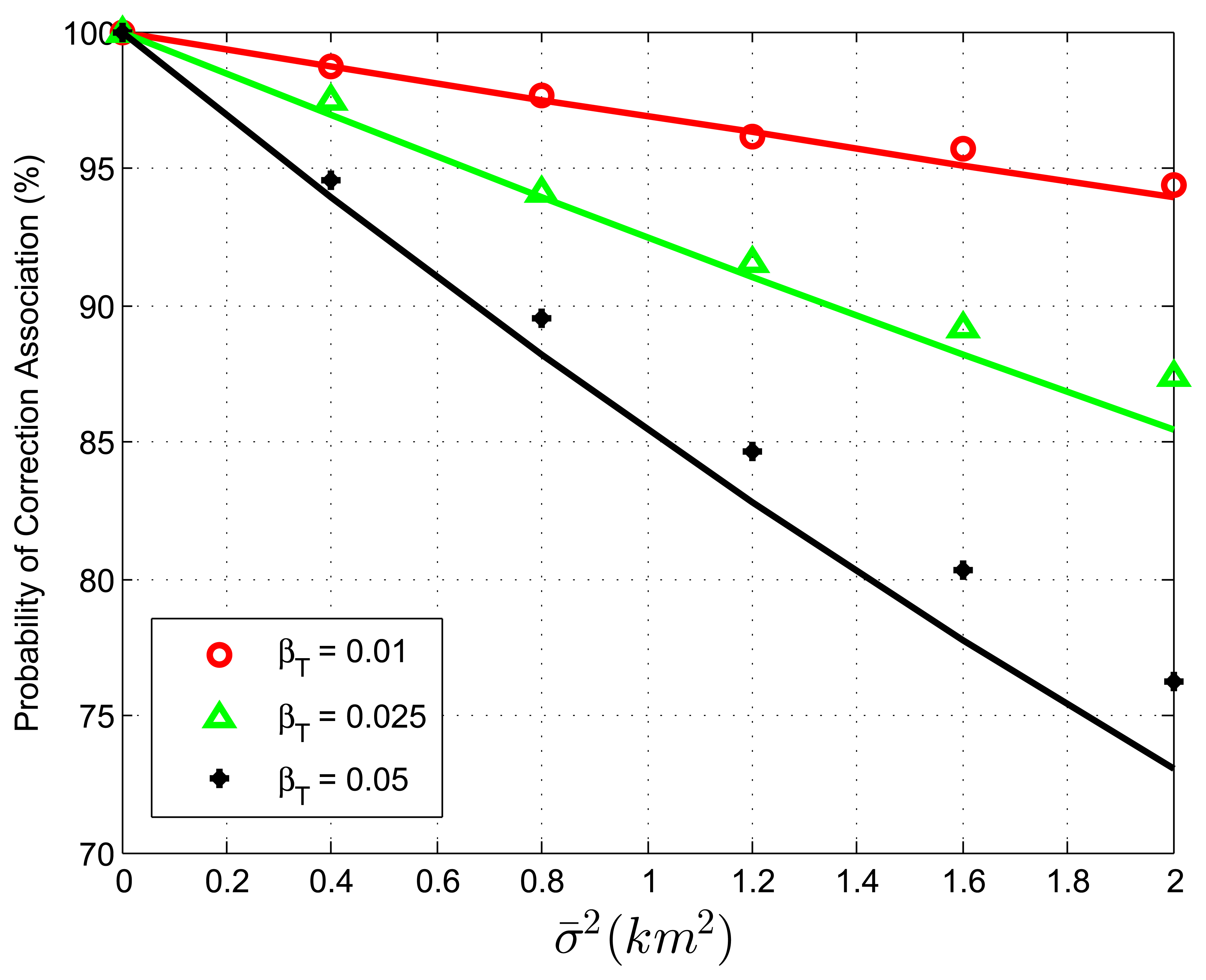
When we study the validity of Equation (42) with biased data and no extraneous tracks, two simulation experiments are designed. The target spatial density, β_T, is set to be 0.01, 0.025, 0.05 reports/km², with the target extent radius r being 25.23, 15.95, 11.28 km, respectively. In the first experiment, the average association uncertainty covariance matrix is fixed to be S = diag[1, 1] km², while Δb_x, Δb_y vary from −3 km to 3 km in increments of 1 km.

Table 1. The impact of sensor biases on correct association probability—the prediction by Equation (42) is 96.90%. β_T = 0.01 reports/km².

PC (%)		Δbx
		−3km	−2km	−1km	0km	1km	2km	3km
Δby	-3 km	96.87	97.16	96.63	97.23	97.48	97.55	97.09
	-2 km	96.85	96.86	97.03	97.23	97.26	97.10	97.06
	-1 km	97.21	96.80	96.37	96.91	96.62	96.95	97.00
	0 km	97.43	97.37	96.79	97.24	97.26	97.43	96.95
	1 km	97.19	97.04	97.67	97.52	97.11	97.16	97.17
	2 km	97.07	97.20	97.17	96.90	97.62	97.67	97.32
	3 km	97.26	97.08	97.28	96.88	97.19	97.17	97.11

,

Table 2. The impact of sensor biases on correct association probability—the prediction by Equation (42) is 92.44%. β_T = 0.025 reports/km².

PC (%)		Δbx
		−3km	−2km	−1km	0km	1km	2km	3km
Δby	-3 km	92.98	93.14	93.07	93.36	93.47	92.96	92.5
	-2 km	93.54	92.98	93.55	93.03	93.25	93.18	93.27
	-1 km	92.87	94.02	92.83	93.15	93.35	92.98	92.21
	0 km	93.03	92.41	93.30	93.21	93.00	93.02	92.89
	1 km	92.14	93.67	92.87	92.95	93.44	93.44	93.92
	2 km	93.17	92.80	92.40	93.11	93.24	92.76	93.15
	3 km	92.87	92.91	93.58	92.83	93.14	93.17	92.77

and

Table 3. The impact of sensor biases on the correct association probability—the prediction by Equation (42) is 85.46%. β_T = 0.05 reports/km².

PC (%)		Δbx
		−3km	−2km	−1km	0km	1km	2km	3km
Δby	-3 km	87.81	86.85	87.20	87.79	86.73	87.03	86.62
	-2 km	87.51	86.83	86.48	87.34	86.31	86.29	87.63
	-1 km	86.88	87.78	86.66	86.63	86.61	87.28	86.25
	0 km	87.24	87.07	86.39	88.13	87.64	86.46	86.98
	1 km	87.17	87.01	87.10	86.63	87.02	86.95	88.18
	2 km	86.73	86.68	86.74	87.27	86.42	87.10	86.86
	3 km	86.48	86.49	87.28	86.85	86.57	87.34	86.71

show that the correct association probability, P_C, obtained by simulations remains approximately unchanged and matches the analytic prediction well, even if the sensor biases vary in a big range. That is because, when no extraneous tracks exist, the P_C of the GNN association algorithm is not associated with translational biases in Equation (42). From the comparison between Tables 1, 2 and 3, the theoretical P_C value given by Equation (42) is less accurate as the track density increases. An explanation of this phenomenon is that, although the assumption of a large enough r is necessary in the derivation of Equation (42), the target extent radius, r, is not large enough under a high target density. Another possible reason might originate from the more complicated association errors, i.e., multi-object transpositions, which we did not model. However, the statistics concerning such “high-order” transpositions are not clear at the moment. In the second experiment, sensor biases are fixed to be Δb_x = Δb_y = 1 km, while the average association variance, σ̄², varies from 0 km² to 2 km² in increments of 0.4 km². Figure 1 plots the correct association probability, P_C, as a function of σ̄², and each point is compared with the prediction (solid line) by Equation (42). The analytic prediction results match the simulation results very well, with a few exceptions: when the targets are dense and the average association variance is large. In view of the approximations we have employed, including some quite “bold” ones, such as the independent transposition assumption, this consistency between the simulation results and the theoretical prediction is rather remarkable.

5.2. Extraneous Tracks Only in One Track Set

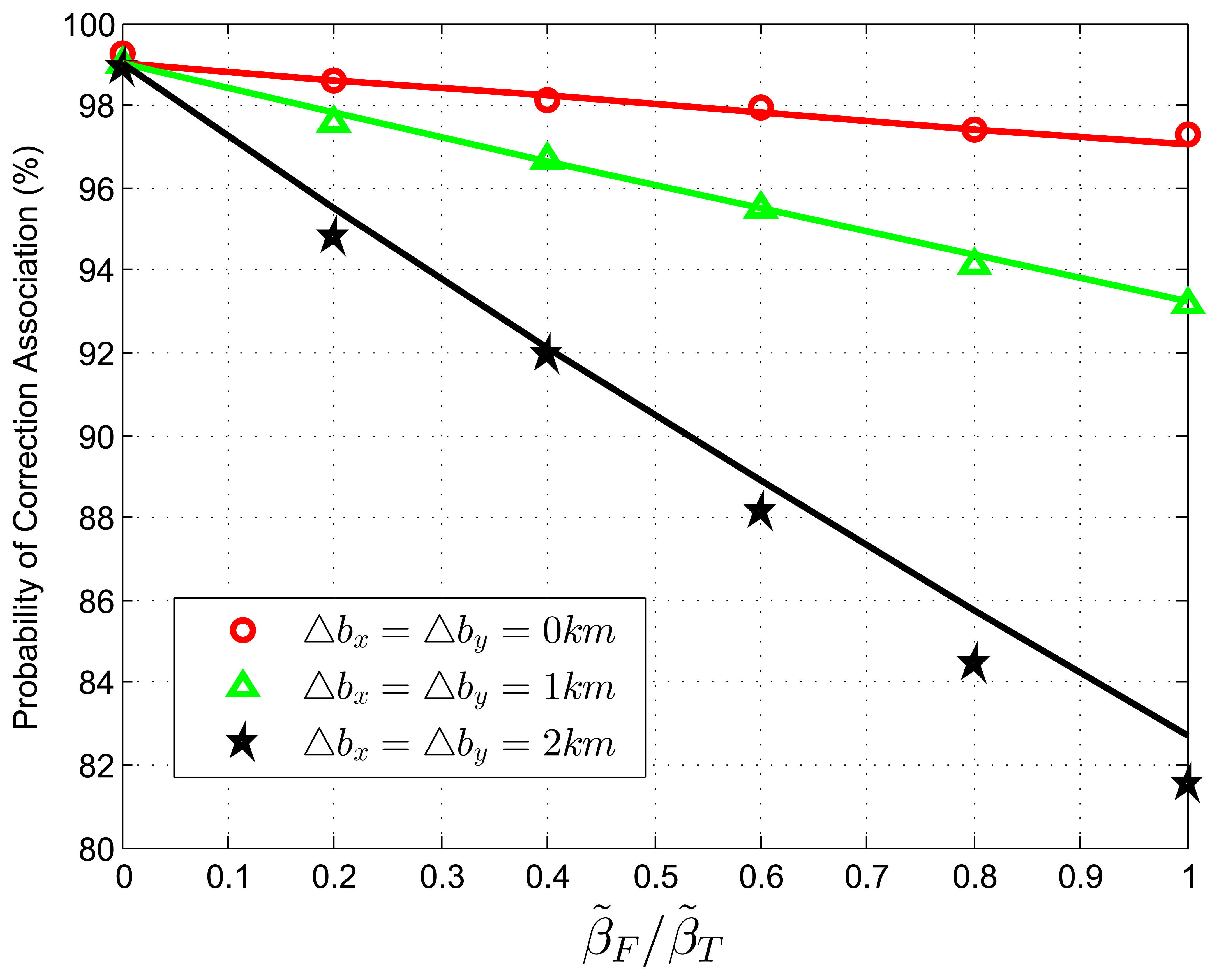
When we test Equation (76) with extraneous tracks in the track set of sensor B, the normalized target density, β˜_T, is fixed to be 0.05 reports, with the average association uncertainty covariance matrix, S = diag[0.5, 0.5] km², and the target extent radius, r = 14.14 km. The relative translational biases are set as Δb_x = Δb_y = 0, 1, 2 km. The ratio, β˜_F/β˜_T, is changed from zero to one in increments of 0.2. In each Monte Carlo run, false tracks are added according to given densities. Figure 2 shows the correct association probability as a function of the ratio, β˜_F/β˜_F, which determines the relative density of extraneous tracks to target tracks. The analytic prediction results (solid lines) match the simulation results (points) very well, and they perform better matching when small sensor biases occur.

5.3. Extraneous Tracks in Both Track Sets

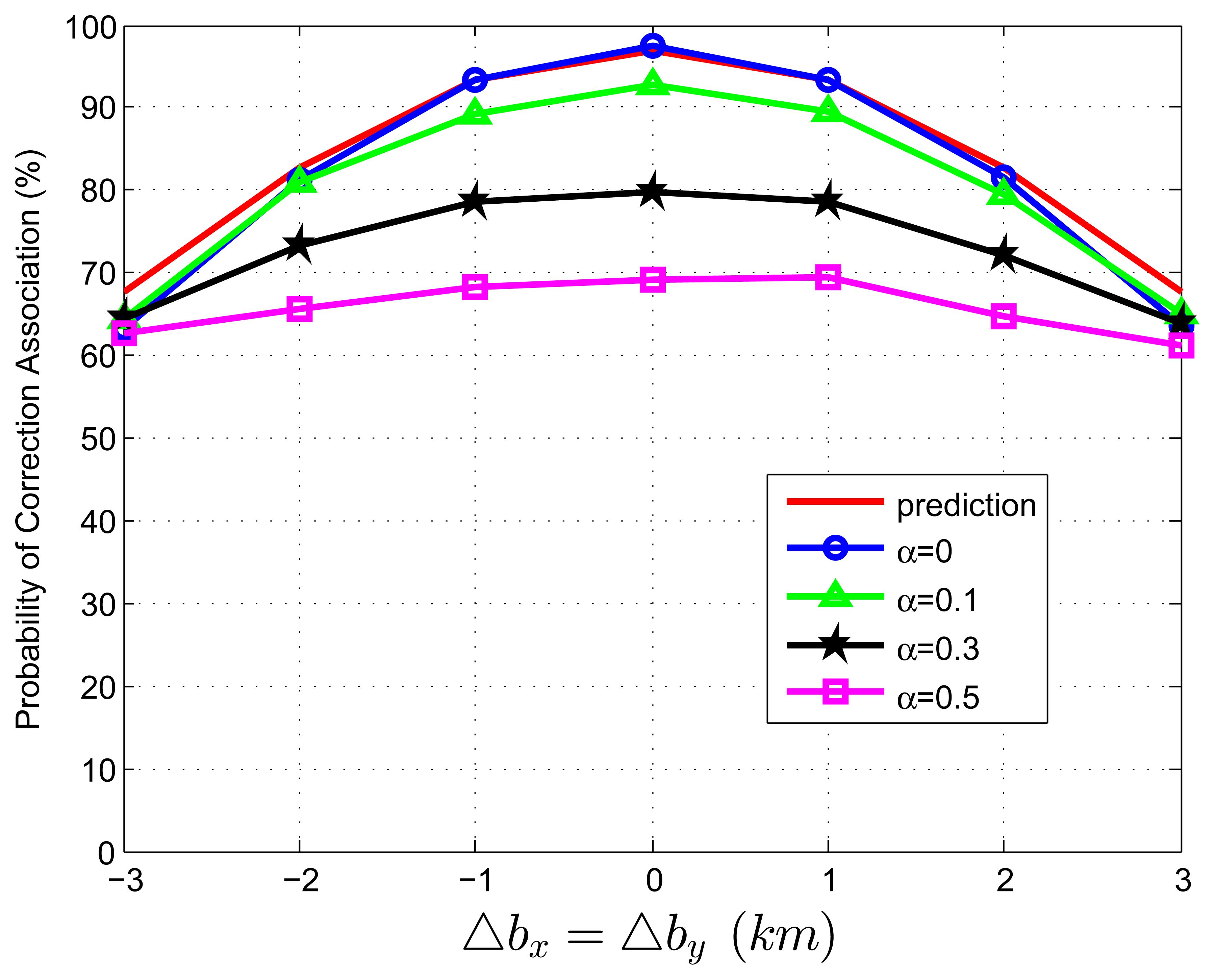
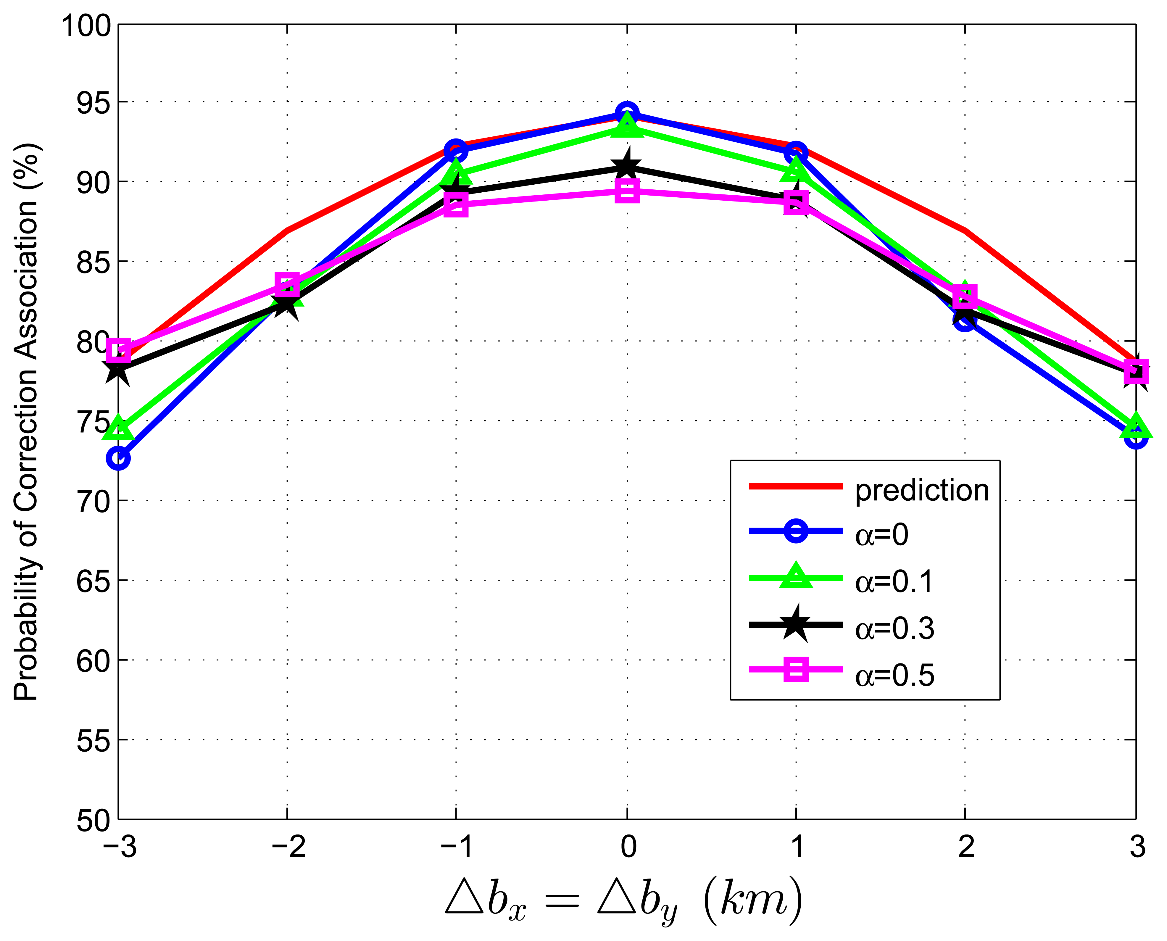
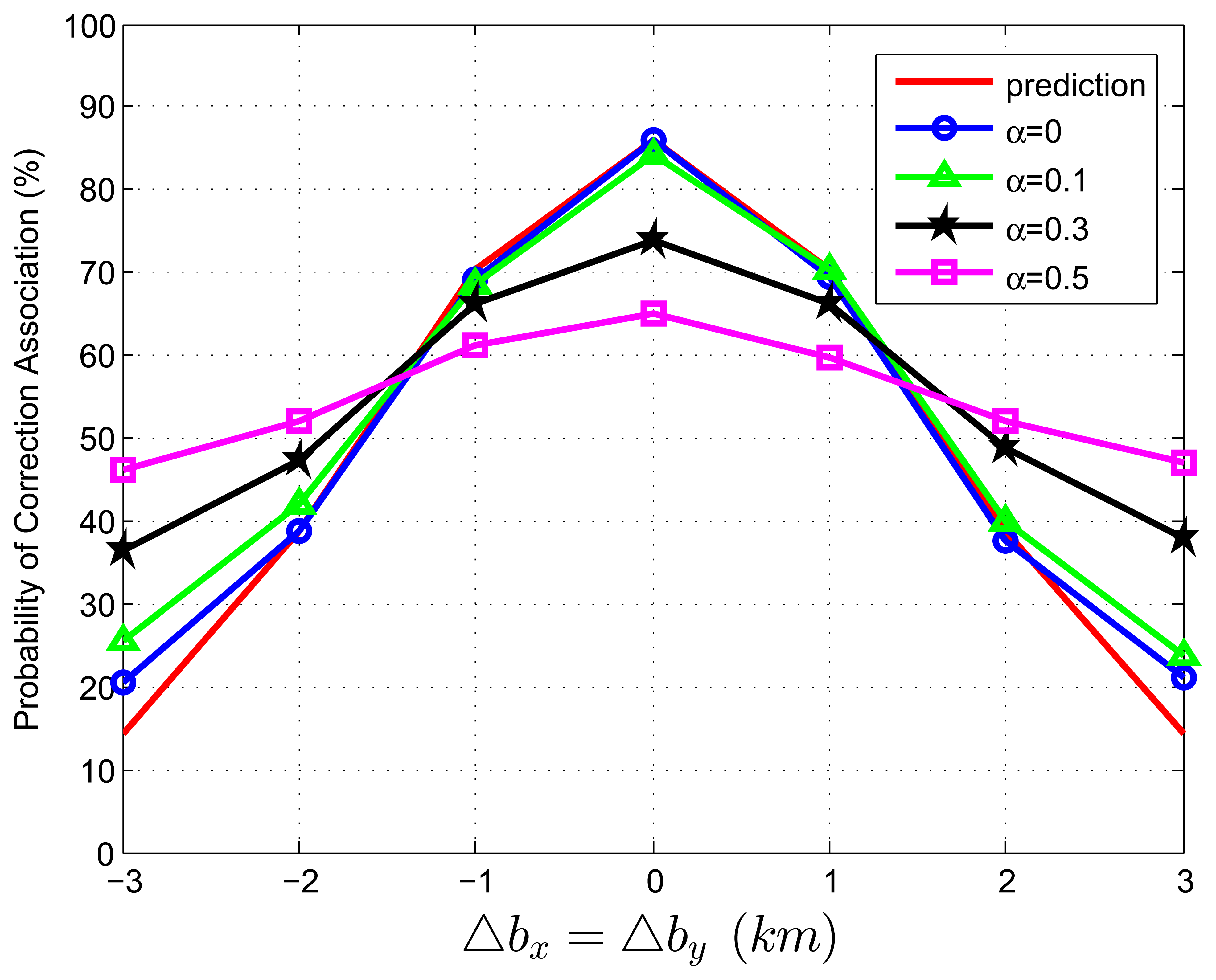
When we test Equation (82) with extraneous tracks in both track sets, the average association covariance matrix is set to be S = diag[0.5, 0.5] km², and Δb_x is assumed to be equal with Δb_y varying from -3 km to 3 km in increments of 1 km. Let β˜_F be the total normalized density of extraneous tracks, and β˜_F = β˜_FA + β˜_FB. Let α be the ratio of false tracks from sensor A, and α = β˜_FA/β˜_F. Given the total density of false tracks, the parameter, α, reflects the allocation (or the relative quantity) of the extraneous tracks between sensor A and B. Four cases of α (α = 0, 0.1, 0.3, 0.5) are considered in the simulations. To better understand the prediction performance of Equation (82), two groups of simulation experiments are performed. In the first group, the normalized target spatial density, β˜_T, is fixed to be 0.01 reports (accordingly, r is set as 31.62 km). Figures 3 and 4 plot the correct association probability as a function of sensor biases, with β˜_F = 0.1β˜_T and β˜_F = β˜_T, respectively. In the second group, β˜_T is fixed to be 0.05 reports (accordingly, r is 14.14 km). Figures 5 and 6 plot the correct association probability as a function of sensor biases, with β˜_F = 0.1β˜_T and β˜_F = β˜_T, respectively.

Since a series of assumptions are made in the derivation of Equation (82), the prediction accuracy degrades in the scenario where false tracks exist in both sensors. When the number of extraneous objects is far less than the number of targets (β˜_F = 0.1β˜_T), the prediction results are an upper bound for the simulation results, and the prediction deviation is below 7%, as shown in Figures 3 and 5. While there are a lot of false tracks (β˜_F = β˜_T) in Figures 4 and 6, Figure 4 shows that, in the sparse-target scenario (β˜_T = 0.01 reports), even with lots of false tracks, Equation (82) can also be used as an upper bound for the simulation results. Comparing Figure 6 with Figures 3, 4 and 5, we can see that this prediction upper bound becomes invalid only in the scenario with a high target density (β˜_T = 0.05 reports), a high false track density (β˜_F = β˜_T) and large sensor biases (| Δb_x| > 1.3km). Meanwhile, the prediction departure becomes larger as α increases. The fundamental reason for the prediction departure is not clear at this point. Two possible explanations are given as follows. First, in this complicated scenario, especially with a large α (≤ 0.5), false tracks of different sensors may associate with each other. This leads to a “reduction” of the false track density. In this sense, β_FA + β_FB in Equation (82) overestimates the density of false tracks. In addition, this false track “reduction” effect can be amplified under large sensor biases, since the multiplying factor, $D_m^{\prime }$, in Equation (82) is a quadratic function of sensor biases. Second, when both track sets have false tracks, the multi-object transpositions we did not model are apt to occur. Yet, for all that, under large sensor biases and a large α (in Figure 6), the extreme pessimistic tendency of the prediction does not matter very much, because it appears only when P_C is quite small (below 50%).

To sum up, in a large range of normally anticipated operating conditions, Equation (82) can be used as an upper bound for the simulation results. Further investigations are needed to provide a more accurate prediction of TTTA in the cases where false tracks exist in both sensors.

6. Conclusion

In this paper, we proposed an analytic performance prediction method for the GNN association algorithm with biased data in multi-sensor multi-target tracking applications. The probability of correct association is adopted as the performance criteria. The novelty of the method lies in that it accounts for the sensor biases in the TTTA problem, and analytic approaches are developed to reveal the intrinsic relationship between a set of key scenario parameters and the performance of the optimal TTTA algorithm. To verify the validity of the predictions, we compared them with the results of Monte-Carlo simulations. These shows that the analytic predictions agree reasonably well with the simulation results. In a word, the main results of the paper are as follows:

(1)

When both track sets are free from extraneous tracks, the correct association probability of the GNN association algorithm in Equation (42) has nothing to do with the translational biases of sensors. It is only related with target spatial density and the average association errors.

(2)

When one track set suffers from extraneous tracks, an exponential law was given in Equation (76), which uncovers the relationship between the correct association probability and the scenario parameters, including the average association errors, sensor biases, the target spatial density, as well as the false track density. The impact of sensor biases is embodied by an amplification coefficient of the false track density.

(3)

When both track sets contain extraneous tracks, an analytic upper bound of the correct association probability for the GNN association algorithm was proposed in Equation (82), which is effective in a large range of scenario parameters.

A series of assumptions were made to get concise and explicit mathematical results, including no missed detection, the translational bias model, identical association uncertainty covariance on all tracks, etc. The results derived based on these assumptions are not intended to be used directly in practice. The major contribution of the paper is to help designers understand the intrinsic relationship between a set of key scenario parameters and the performance of TTTA and to demonstrate the possibility that analytic performance prediction can be a potential substitute for the costly Monte Carlo simulation method.

To make the proposed analytic method more practical, a lot of work is needed in the following directions:

(1)

Further investigations are needed to improve the prediction accuracy of our method in the scenario where false tracks exist in both sensors. The statistics concerning the more complicated association error,s such as multi-object transpositions, can be addressed in the future.

(2)

For simplicity, we assumed that the track detection probabilities of both sensors are one. However, missed detections and false tracks do happen in real environments. To complicate matters, when missed detections occur at one sensor, the corresponding tracks that are supposed to associate with these missed tracks in the track set of the other sensor are equivalent to extraneous tracks for the remaining tracks of the former sensor. When sensors suffer from both missed detections and extraneous tracks, accounting for the missed detections in the formula of the correct association probability needs to be investigated in the future.

(3)

We only examined the impact of translational biases on the performance of TTTA. Since the impact of translational biases on the tracks is uncoupled with the states of targets, the translational biases can be named state-independent biases. However, in some applications, sensors can have biases on their range and azimuth measurements. The impact of these biases on the position estimates of targets is dependent on the real states of targets. Therefore, we name the range and azimuth biases the state-dependent biases. Under the scenario with state-dependent biases, the bias terms cannot be canceled out in Equations (24) and (25). Thus, the state-dependent biases affect the performance of the GNN association algorithm, even if there are no false tracks and missed detections. How to deal with the more complicated state-dependent biases in analytic performance prediction is left for the future.

References

- Blackman, S.S.; Popoli, R. Design and Analysis of Modern Tracking Systems; Artech House: Norwood, MA, USA, 1999. [Google Scholar]
- Bar-Shalom, Y.; Willett, P.K.; Tian, X. Tracking and Data Fusion; YBS publishing: Storrs, CT, USA, 2011. [Google Scholar]
- Sea, R.G. An Efficient Suboptimal DecisionProcedure for Associating Sensor Data with Stored Tracks in Real-Time Surveillance Systems. Proceeding of 1971 IEEE Conference on Decision and Control, Miami Beach, FL, USA, December 1971; pp. 33–37.
- Singer, R.; Sea, R.G. New results in optimizing surveillance system tracking and data correlation performance in dense multitarget environments. IEEE Trans. Autom. Control 1973, 18, 571–582. [Google Scholar]
- Saha, R.K. Analytical Evaluationof an Esm/Radar Track Association Algorithm. Proceeding of Signal and Data Processing of Small Targets, Orlando, FL, USA, April 1992; pp. 338–347.
- Li, X.R.; Bar-Shalom, Y. Tracking in clutter with nearest neighbor filters: Analysis and performance. IEEE Trans. Aerosp. Electron. Sys. 1996, 32, 995–1010. [Google Scholar]
- Mei, W.; Shan, G. Performance of a multiscan track-to-track association technique. Signal Process. 2005, 85, 1493–1500. [Google Scholar]
- Mori, S.; Chang, K.C.; Chong, C.Y. Performance analysis of optimal data association with applications to multiple target tracking. Multitarg. Multisens. Track. Appl. Adv. 1992, 2, 183–235. [Google Scholar]
- Mori, S.; Chang, K. C.; Chong, C.Y.; Dunn, K.P. Prediction of track purity and track accuracy in dense target environments. IEEE Trans. Autom. Control 1995, 40, 953–959. [Google Scholar]
- Ruan, Y.; Hong, L.; Wicker, D. Analytic performance prediction of feature-aided global nearest neighbour algorithm in dense target scenarios. IET Radar Sonar Navig. 2007, 1, 369–376. [Google Scholar]
- Areta, J.A.; Bar-Shalom, Y.; Rothrock, R. Misassociation probability in M2TA and T2TA. J. Adv. Inf. Fusion 2007, 2, 113–127. [Google Scholar]
- Areta, J.A.; Bar-Shalom, Y.; Rothrock, R. The Probability of Misassociation Between Neighboring Targets. Proceedings of Signal and Data Processing of Small Targets, Orlando, FL, USA, 16 March 2008; pp. 69691B:1–69691B:11.
- Mori, S.; Chong, C.Y.; Chang, K.C. Performance Prediction of Feature Aided Track-to-Track Association. Proceedings of the 14th International Conference on Information Fusion (FUSION 2011), Chicago, IL, USA, 5–8 July 2011; pp. 1–8.
- Chen, S.; Leung, H.; Bosse, E. A Maximum Likelihood Approach to Joint Registration, Association and Fusion for Multi-Sensor Multi-Target Tracking. Proceeding of 12th International Conference on Information Fusion (FUSION 2009), Seattle, WA, USA, 6–9 July 2009; pp. 686–693.
- Li, Z.; Chen, S.; Leung, H.; Bosse, E. Joint data association, registration, and fusion using em-kf. IEEE Trans. Aerosp. Electron. Sys. 2010, 46, 496–507. [Google Scholar]
- Moy, G.; Blaty, D.; Farber, M.; Nealy, C. Fusion of Radar and Satellite Target Measurements. Proceeding of Sensors and Systems for Space Applications IV, Orlando, FL, USA, 16 May 2011; pp. 804405–804405.
- Papageorgiou, D.J.; Sergi, J.D. Simultaneous Track-to-Track Association and Bias Removal Using Multistart Local Search. Proceeding of IEEE Aerospace Conference, Big Sky, MT, USA, 1–8 March 2008; pp. 1–14.
- Danford, S.; Kragel, B.; Poore, A. Joint Map Bias Estimation and Data Association: Algorithms. Proceeding of Signal and Data Processing of Small Targets, San Diego, CA, USA, 26 August 2007; pp. 66991E:1–66991E:18.
- Levedahl, M. Explicit Pattern Matching Assignment Algorithm. Proceedings of Signal and Data Processing of Small Targets, Orlando, FL, USA, 1 April 2002; pp. 461–469.
- Deb, S.; Yeddanapudi, M.; Pattipati, K.; Bar-Shalom, Y. A generalized sd assignment algorithm for multisensor-multitarget state estimation. IEEE Trans. Aeros. Electron. Sys. 1997, 33, 523–538. [Google Scholar]
- Pattipati, K.R.; Kirubarajan, T.; Popp, R.L. Survey of assignment techniques for multitarget tracking. Multitarg. Multisens. Track. Appl. Adv. 2000, 3, 77–159. [Google Scholar]
- Hurley, M.B. Track Association with Bayesian Probability Theory; Technical Report 1085; Massachusetts Institute of Technology Lincoln Laboratory: Cambridge, MA, USA; October; 2003. [Google Scholar]
- Kaplan, L.; Bar-Shalom, Y.; Blair, W. Assignment costs for multiple sensor track-to-track association. IEEE Trans. Aeros. Electron. Syst. 2008, 44, 655–677. [Google Scholar]
- Blair, W.D.; Kaplan, L.M. Assignment Costs for Multiple Sensor Track-to-Track Association. Proceeding of Seventh International Conference on Information Fusion (Fusion 2004), Stockholm, Sweden, 28 June–1 July 2004.
- Bourgeoism, F.; Lassalle, J.C. An extension of the munkres algorithm for the assignment problem to rectangular matrices. Commun. ACM 1971, 14, 802–804. [Google Scholar]
- Jonker, R.; Volgenant, A. A shortest augmenting path algorithm for dense and sparse linear assignment problems. Computing 1987, 38, 325–340. [Google Scholar]
- Castañón, D.A. New assignment algorithms for data association. Proceedings of Signal and Data Processing of Small Targets, Orlando, FL, USA, 20 April 1992; pp. 313–323.
- Castella, F.R. Theoretical Performance of a Multisensor Track-to-Track Correlation Technique. Proceeding of IEE Radar Sonar Navigation, December 1995; pp. 281–285.
- Singer, R.A.; Kanyuck, A.J. Computer control of multiple site track correlation. Automatica 1971, 7, 455–463. [Google Scholar]
- Tian, X.; Bar-Shalom, Y. Sliding Window Test vs. Single Time Test for Track-to-Track Association. Proceeding of 11th International Conference on Information Fusion (Fusion 2008), Cologne, Spain, 30 June–3 July 2008; pp. 1–8.
- Tian, X.; Bar-Shalom, Y. Track-to-track fusion configurations and association in a sliding window. J. Adv. Inf. Fusion 2009, 4, 146–164. [Google Scholar]
- Mori, S.; Chong, C.Y. Effects of Unpaired Objects and Sensor Biases on Track-to-Track Association: Problems and Solutions. Proceedings of MSS National Symposium on Sensor and Data Fusion, San Antonio, TX, USA, 20–22 June 2000; pp. 137–151.
- Bar-Shalom, Y.; Li, X.R. Multitarget-Multisensor Tracking: Principles and Techniques; University of Connecticut: Storrs, CT, USA, 1995. [Google Scholar]
- Bar-Shalom, Y.; Chen, H. Multisensor track-to-track association for tracks with dependent errors. J. Adv. Inf. Fusion 2006, 1, 2674–2679. [Google Scholar]
- Soule, P.W. Performance of Two-way Association of Complete Data Sets.; No. TOR0074(4085)-15; Aerospace Corp.: El Segundo, CA, USA; January; 1974. [Google Scholar]
- Kay, S.M. Fundamentals of Statistical Signal Processing, Volume 2: Detection Theory; Prentice Hall PTR: London, UK, 1998. [Google Scholar]
- Harvey, J.R. Fractional Moments of a Quadratic Form in Noncentral Normal Random Variables. PhD. Thesis, North Carolina State University, April 1965. [Google Scholar]
- Fortmann, T.E.; Bar-Shalom, Y.; Scheffe, M.; Gelfand, S. Detection Thresholds for Multi-Target Tracking in Clutter; No. 5495; BBN Laboratory. Inc.: Cambridge, MA, USA; December; 1983. [Google Scholar]