The Control of Tendon-Driven Dexterous Hands with Joint Simulation

Abstract

An adaptive impedance control algorithm for tendon-driven dexterous hands is presented. The main idea of this algorithm is to compensate the output of the classical impedance control by an offset that is a proportion-integration-differentiation (PID) expression of force error. The adaptive impedance control can adjust the impedance parameters indirectly when the environment position and stiffness are uncertain. In addition, the position controller and inverse kinematics solver are specially designed for the tendon-driven hand. The performance of the proposed control algorithm is validated by using MATLAB and ADAMS software for joint simulation. ADAMS is a great software for virtual prototype analysis. A tendon-driven hand model is built and a control module is generated in ADAMS. Then the control system is built in MATLAB using the control module. The joint simulation results demonstrate fast response and robustness of the algorithm when the environment is not exactly known, so the algorithm is suitable for the control of tendon-driven dexterous hands.

1. Introduction

The control system of dexterous robot hands can control the robot fingers to reach the desired position, contact with the environment and track a specified desired force. Thereinto, stable force tracking is an important research topic, which can be solved by compliance control. Impedance force control is very practical in the field of robotic compliance control and the main concept is based on the impedance equation which is the relationship between force and position/velocity error [1].

Many researchers have improved the performance of the impedance control and expanded the application range since it was primarily proposed by Hogan [2–5]. However, the classical impedance control is unsatisfying when the environment parameters are not exactly known. To overcome this problem, Lasky et al. [6] proposed a two-loop control system that the inner-loop is a classical impedance controller and the outer-loop is a trajectory modified for force-tracking. This algorithm uses the outer-loop to automatically modify the reference position by a simple force-feedback scheme when the environment is not exactly known. Jung et al. [1] proposed an adaptive impedance control. The main idea of this algorithm is to minimize the force error directly by using a simple adaptive gain when the environment is changed. Seraji [7] proposed an adaptive admittance control based on the concept of mechanical admittance, which relates the contact force to the resulting velocity perturbation. Two adaptive PID and PI force compensators are designed in Seraji's paper.

In this paper an adaptive impedance control is proposed that uses an adaptive PID force compensator as an offset to adjust the output of the impedance controller when the environment position or stiffness is changed. It is a way that adjusts the impedance parameters indirectly, which is different from Jung's. In order to validate the algorithm, a joint simulation with MATLAB and ADAMS is presented. Firstly, the model of the tendon-driven dexterous hand is built in ADAMS referring to the robot hand of Robonaut-2, which is the first humanoid robot in space and has the typical tendon-driven dexterous hands [8]. A three-DOF finger of the robot hand is chosen as the research object. Then a control module of the robot finger is generated in ADAMS. Finally, the control system is built in MATLAB using the control module. The results of the joint simulation demonstrate that the proposed algorithm is robust. In addition, the position controller and inverse kinematics solver are designed for the tendon-driven finger.

2. Features of the Robot Hand and Dynamic Model

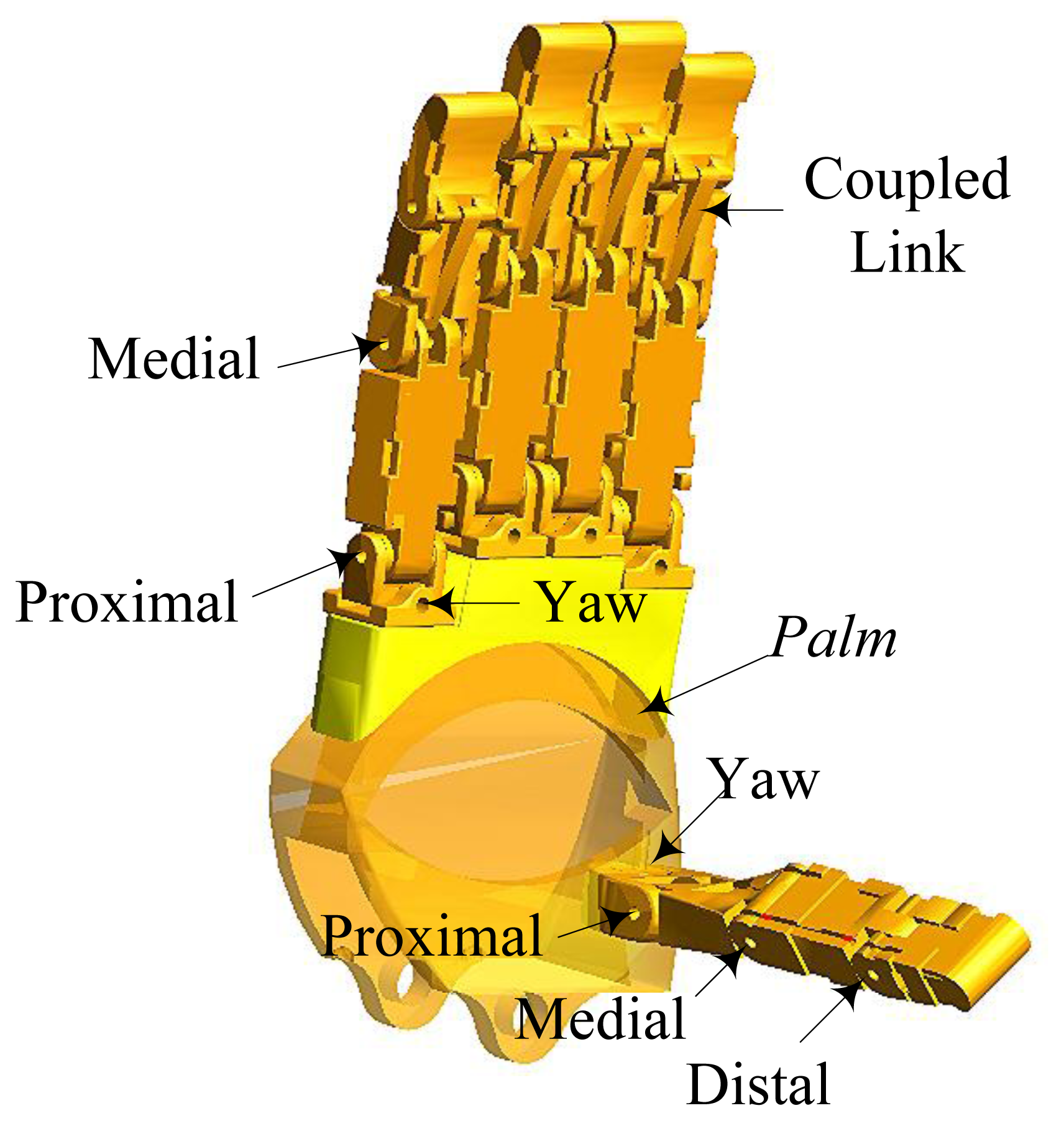
The model of the tendon-driven dexterous hand in ADAMS consists of four three-DOF fingers, a four-DOF thumb and a palm, as shown in Figure 1. For the three-DOF fingers, the fingertip's motion depends on the coupled link, as shown in Figure 1. The actuation system of the robot hand is remotely packaged in the forearm, which makes the size of the robot hand as large as a man's hand. Each unit of the actuation system consists of a brushless motor and a lead screw. The lead screw can convert rotary motion to linear motion. Each of the tendons connects the finger joint and the lead screw. The motors can drive the lead screws to control the finger motion through the tendons. Since the tendons can only transmit forces in tension, the number of tendons should be more than the DOFs. It turns out that only one tendon more than the number of DOF is needed [9], so a three-DOF finger needs four tendons.

The dynamic model of the three-DOF finger can be expressed as follows:

$$\mathit{M}(\mathit{q})\ddot{\mathit{q}}+\mathit{C}(\mathit{q},\dot{\mathit{q}})\dot{\mathit{q}}+\mathit{g}(\mathit{q})=\mathit{\tau }‐{\mathit{\tau }}_{\text{f}}+{\mathit{\tau }}_{\text{ext}}$$

(1)

where M(q), C(q) and g(q) represent the inertia matrix, centrifugal term, and gravity term respectively; q represents the joint angle vector; τ, τ_f and τ_ext represent the joint torque vector, friction torque vector and external torque vector respectively. τ_ext is given by [10]:

$${\mathit{\tau }}_{\text{ext}}={\mathit{J}}^T{\mathit{F}}_t$$

(2)

where J represents the Jacobian matrix, F_t = [ F_tx F_ty F_tz]^T represents the fingertip force. τ_m is defined as the motor torque vector. Then there should be a certain relationship between τ and τ_m, which is shown as follow.

Firstly, for the three-DOF finger, the transformation from four tensions to three joint torques is given by [9,10]:

$$\mathit{\tau }=\mathit{R}\mathit{f},\mathit{R}=\left[\begin{array}{cccc}{r}_{11}& r_{12}& -r_{13}& -r_{14}\\ r_{21}& -r_{22}& r_{23}& -r_{24}\\ 0& 0& r_{33}& -r_{34}\end{array}\right]$$

(3)

where f is a column vector consisting of four tendon tensions; R represents the mapping from tensions (f) to joint torques (τ) and r_ij is the radius of the circular surface where the j-tendon envelops itself on the i-joint (The tendons are numbered from t₁ to t₄, as shown in Figure 2), i = 1 ∼ 3, j = 1 ∼ 4. For the three-DOF finger, r₁₁ = r₁₂ = r₁₃ = r₁₄ = 5.5 mm, r₂₁ = r₂₂ = r₂₃ = r₂₄ = 5.2 mm, r₃₃ = r₃₄ = 5.0 mm.

Secondly, the relationship between the tendon tensions and motor torques is expressed as:

$$\mathit{f}=\frac{2\pi }{d}{\mathit{\tau }}_{\text{m}}$$

(4)

where d represents the screw pitch of the lead screws.

According to Equations (3) and (4), the Equation (1) can be rewritten as:

$$\mathit{\text{M}}(\mathit{\text{q}})\ddot{\mathit{q}}+\mathit{\text{C}}(\mathit{\text{q}},\dot{\mathit{\text{q}}})\dot{\mathit{q}}+\mathit{\text{g}}(\mathit{q})=\frac{2\pi }{d}\mathit{R}{\mathit{\tau }}_{\text{m}}\mathit{‒}{\mathit{\tau }}_{\text{f}}+{\mathit{\tau }}_{\text{ext}}$$

(5)

The above indicates that the tendons have an impact on the control of the tendon-driven robot hand. In order to simulate the performance of the tendons in ADAMS, the tendon model is built by adding bushing force between small stiffness cylinders. The force analysis between a two small cylinders is shown in Figure 2.

The dynamic equation of the tendon model can be expressed as [11]:

$$\left[\begin{array}{c}\mathit{F}\\ \mathit{T}\end{array}\right]=\mathit{K}\left[\begin{array}{c}\mathit{R}\\ \mathit{\theta }\end{array}\right]-\mathit{C}\left[\begin{array}{c}\mathit{V}\\ \mathit{\omega }\end{array}\right]+\left[\begin{array}{c}{\mathit{F}}_0\\ {\mathit{T}}_0\end{array}\right]$$

(6)

where F and T represent the force and torque between the cylinders respectively; K and C represent the stiffness diagonal matrix and damping diagonal matrix respectively; R, θ, V and ω represent the relative displacement, angle, velocity and angular velocity between the two cylinders respectively; F₀ and T₀ are respectively the initial values of the force and torque. In order to get a reasonable tendon model, K and C should be set to appropriate values. In the control of the robot hand, the tendons that are not flexible enough will affect the finger motion but the very flexible tendons will diminish the control accuracy. Considering that, the satisfying tendon models are built by adjusting the parameters of K and C in ADAMS [12], as shown in Figure 3.

3. The Control System of Tendon-Driven Dexterous Finger

3.1. The Components of the Control System

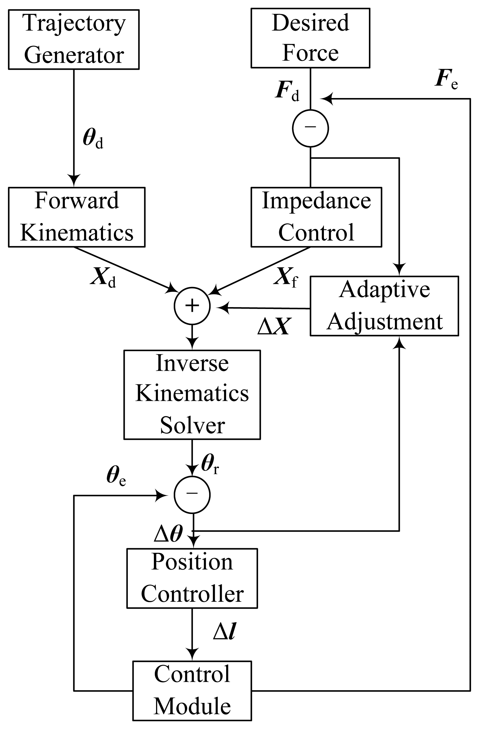
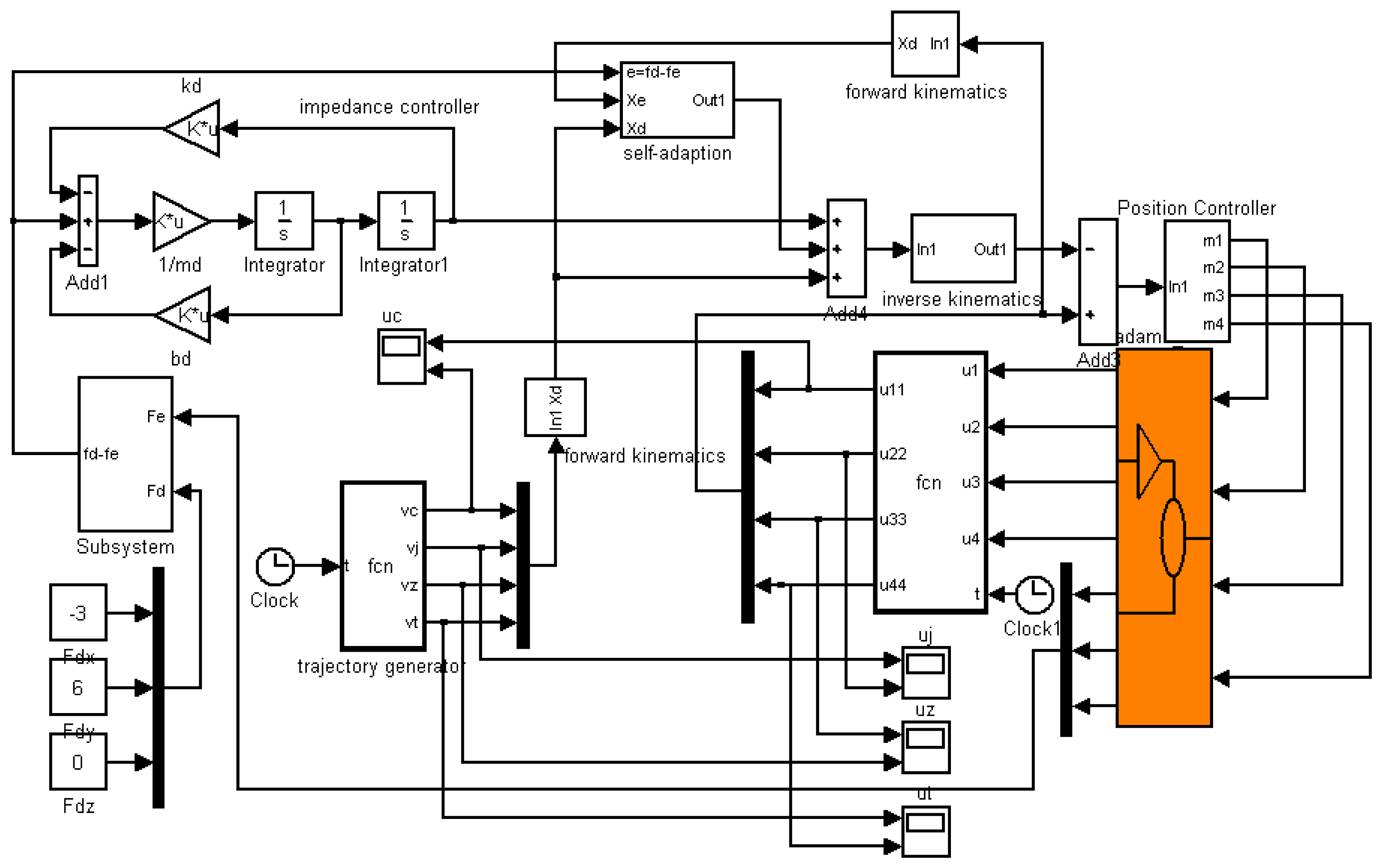
The control system is built for the three-DOF finger. It consists of a control module, adaptive impedance controller, trajectory generator, inverse kinematics solver, position controller and other modules as shown in Figure 4.

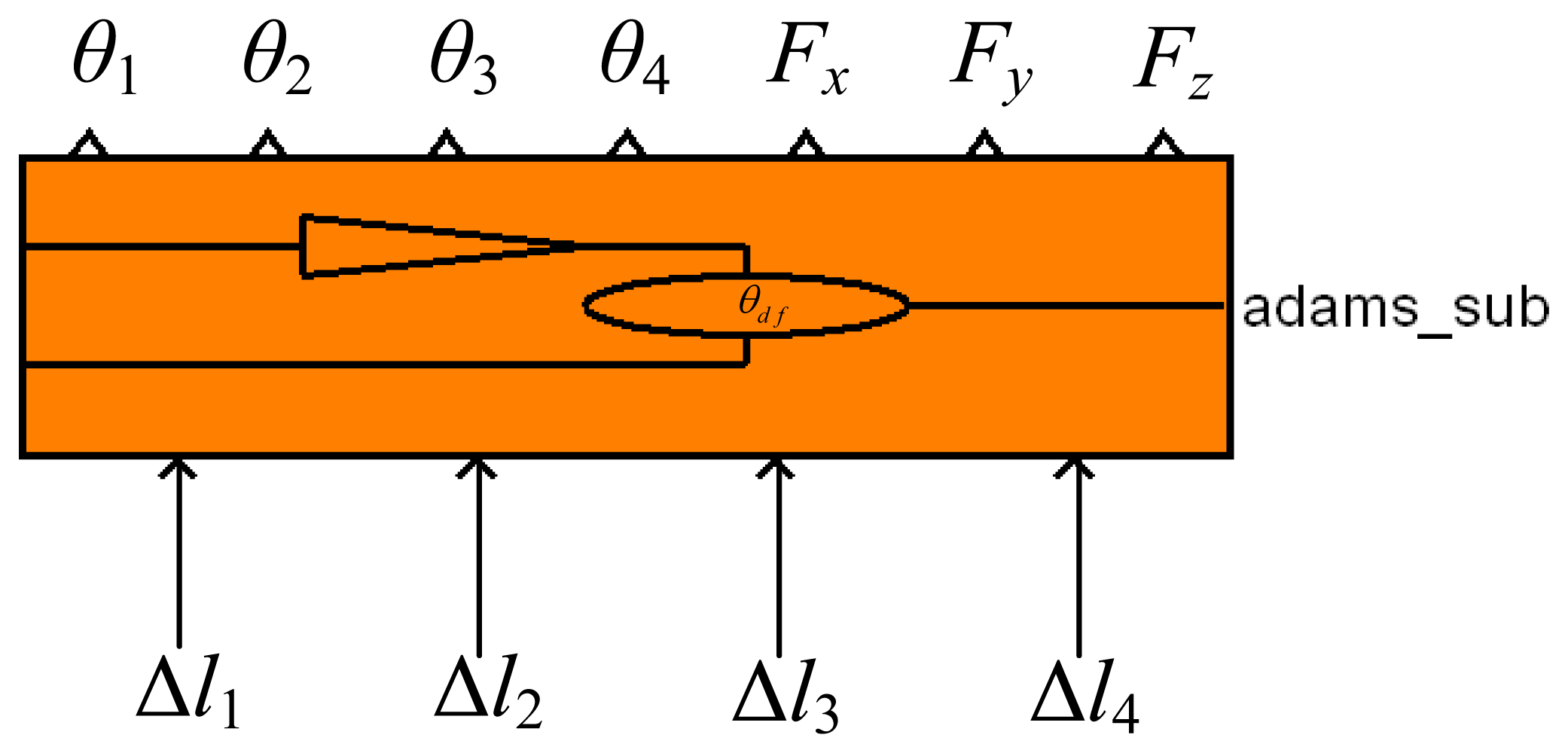
The trajectory generator provides the desired angular displacement θ_d, which need to be converted to the desired displacement X_d in Cartesian-space by forward kinematics because the output of the adaptive impedance controller is in Cartesian-space. The adaptive impedance controller consists of an impedance control part and an adaptive adjustment part. The input of the impedance control part is the difference between the desired contact force F_d and the actual contact force F_e and the output is a displacement offset X_f. And ΔX is defined as the output of the adaptive adjustment part. X_r = X_d + X_f + ΔX represents the displacement that has been adjusted in Cartesian-space. X_r can be converted to the angular displacement θ_r in joint-space by inverse kinematics. Δθ represents the difference between θ_r and the actual angular displacement θ_e. The position controller can convert Δθ to the tendon displacement offset Δl. The control module is generated in ADAMS. It is the interface between ADAMS and MATLAB and contacts the robot model in ADAMS with the control system in MATLAB. So it can be seen as a MATLAB module that has the same effect with the model in ADAMS. The control module of the three-DOF finger is shown in Figure 5 (by the way, θ_d, θ_e, θ_r, Δθ and Δl are four-dimensional column matrices; X_d, X_f, X_r, ΔX, F_d and F_e are three-dimensional column matrices.)

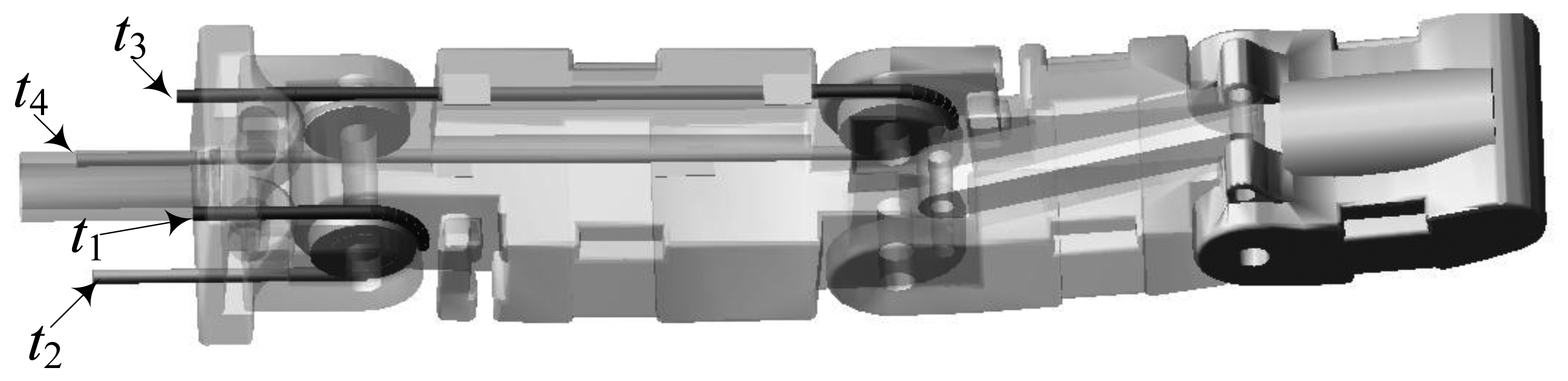
In Figure 5, Δl₁, Δl₂, Δl₃ and Δl₄ are the input variables of the control module and represent the displacement offset of the four tendons; θ₁, θ₂, θ₃, θ₄, F_x, F_y and F_z are the output variables, where θ₁, θ₂, θ₃ and θ₄ represent the angular displacements of joints and F_x, F_y and F_z represent the components of the contact force.

3.2. Adaptive Impedance Controller

The impedance control is based on the concept that it is neither position nor force that should be controlled, but rather the dynamic relation between the two [13]. The relation is an impedance equation, which is given by:

$${\text{M}}_{\text{d}}({\ddot{X}}_{\text{r}}-{\ddot{X}}_{\text{d}})+{\text{B}}_d({\dot{X}}_r-{\dot{X}}_d)+K_d(X_r-X_d)=E$$

(7)

where E = F_d − F_e; M_d, B_d and K_d are respectively 3 × 3 constant-positive-diagonal matrices of the desired inertial, damping and stiffness. The impedance parameters M_d, B_d and K_d should keep the system in the critical damping state or overdamping state at least. And increasing M_d will result in large impact to environment. A large B_d can increase the response time and have no vibration. For position accurate tracking, a large K_d should be selected [14]. According to these, the suitable impedance parameters for specified control system can be got.

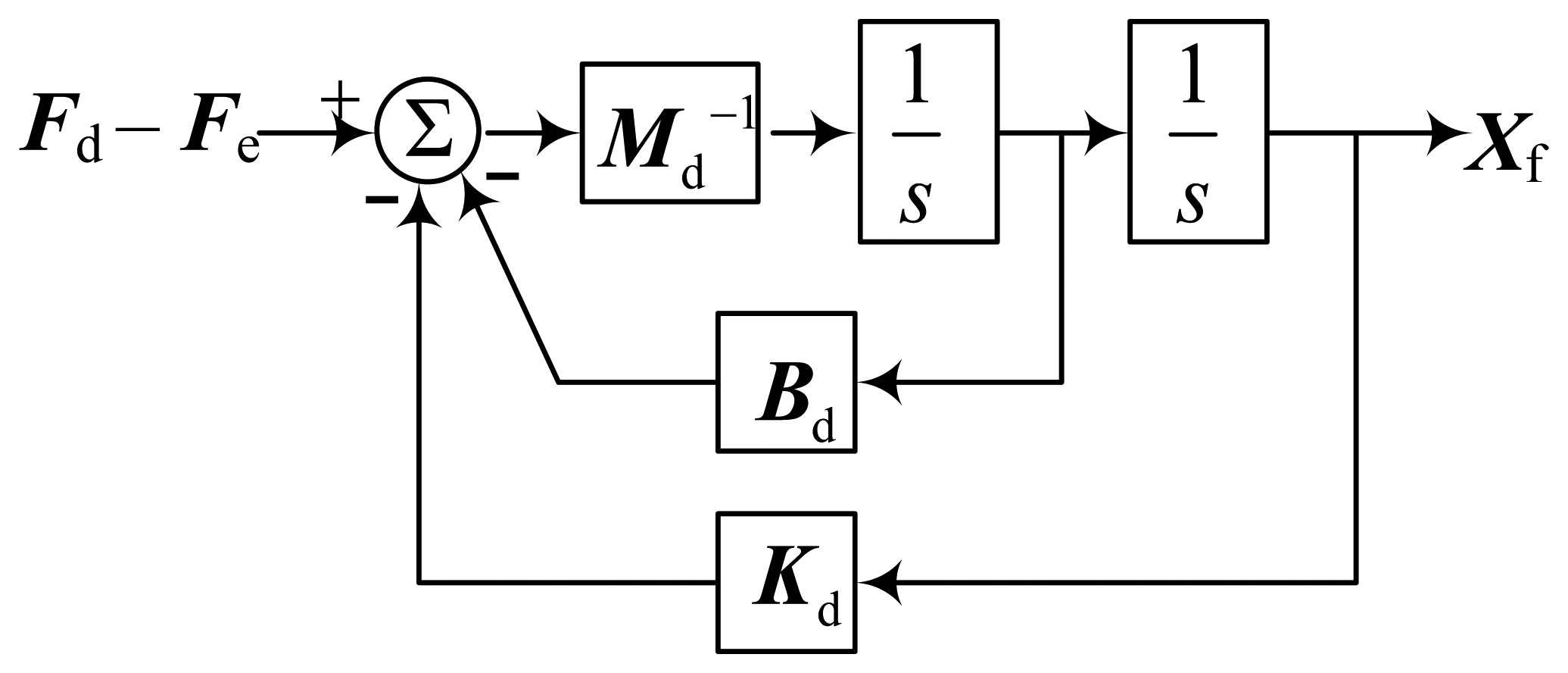
For a classical impedance control, ΔX = 0 and X_f = X_r − X_d. So, Equation (7) can be expressed in the Laplace domain as follows:

$${\mathit{X}}_{\text{f}}(s)=\frac{\mathit{E}(s)}{{\mathit{M}}_d{s}^2+{\mathit{B}}_{d}s+{\mathit{K}}_d}$$

(8)

According to Equation (8), the structure diagram of the impedance control compensator is shown in Figure 6. However, the impedance control compensator is only suitable for a specific environment and the impedance parameters can't be changed in the whole control process. If the environmental parameters changed or weren't exact, the performance of the controller would be unsatisfactory. Hence an adaptive adjustment is needed to change the impedance parameters indirectly according to the environment changes.

The key of the adaptive adjustment is to get an adaptive offset ΔX to compensate the output of the impedance control. Let Δx_k, f_dk, f_ek, x_ek and x_dk respectively represent the k-th element of ΔX, F_d, F_e, X_e, X_d (k = 1–3, X_e represents the actual position of the fingertip in Cartesian-space). Then Δx_k can be expressed as follows [7]:

$$\mathrm{\Delta }{x}_k=g(t)+k_p(t)e(t)+k_d(t)\dot{e}(t)$$

(9)

where g(t) is an auxiliary signal which contains the integral term; k_p(t) and k_d(t) are respectively the adaptive proportional and derivative force feedback gain; e(t) = f_dk − f_ek. Equation (9) is a PID expression of force error in nature, so this adaptive adjustment compensator can respond quickly to the change of the force error, that is to say, to the change of the environment. It is the reason why this expression is used as the compensator of impedance control. g(t), k_p(t) and k_d(t) are given by:

$$\begin{array}{c}q(t)={\omega }_{p}e(t)+{\omega }_d\dot{e}(t)\\ g(t)=g_0+{\alpha }_1{\int }_0^{t}q(t)dt+{\alpha }_{2}q(t)\\ k_p(t)=k_{p0}+{\beta }_1{\int }_0^{t}q(t)e(t)dt+{\beta }_{2}q(t)e(t)\\ k_d(t)=k_{d0}+{\gamma }_1{\int }_0^{t}q(t)\dot{e}(t)dt+{\gamma }_{2}q(t)\dot{e}(t)\end{array}$$

(10)

where ω_p and ω_d are the positive position and velocity weighting factors respectively; α₁, β₁ and γ₁ are the positive integral adaptation gains respectively; α₂, β₂ and γ₂ are the positive or zero proportional adaptation gains. Let α₂, β₂ and γ₂ equal to zero to simplify the expressions. And k_d0, k_p0 and g₀ are the initial values and equal to zero. Since the actual contact force is measured by the force sensor, there is often a noisy signal. Therefore the derivative of the force error is unsatisfying. To solve this problem, ė(t) is replaced by −k_eẋ(t) in Equations (9) and (10), where x(t) = x_dk − x_ek and k_e is a positive constant. In addition, σ-modification terms are used to modify the adaptive compensator to ensure the robustness of the control system [7,15]. Finally the modified expressions of the compensator are given by:

$$\begin{array}{c}\mathrm{\Delta }{x}_k=g(t)+k_p(t)e(t)-k_v\dot{x}(t)\\ q(t)={\omega }_{p}e(t)-{\omega }_v\dot{x}(t)\\ g(t)=g_0+{\alpha }_1{\int }_0^{t}q(t)dt-{\sigma }_1{\int }_0^{t}g(t)dt\\ k_p(t)=k_{p0}+{\beta }_1{\int }_0^{t}q(t)e(t)dt-{\sigma }_2{\int }_0^t{k}_p(t)dt\\ k_v(t)=k_{v0}-{\lambda }_1{\int }_0^{t}q(t)\dot{x}(t)dt-{\sigma }_3{\int }_0^t{k}_v(t)dt\end{array}$$

(11)

where λ₁ = γ₁k_e, ω_v = ω_dk_e; σ₁, σ₂ and σ₃ are small positive constants.

3.3. Inverse Kinematics Solver

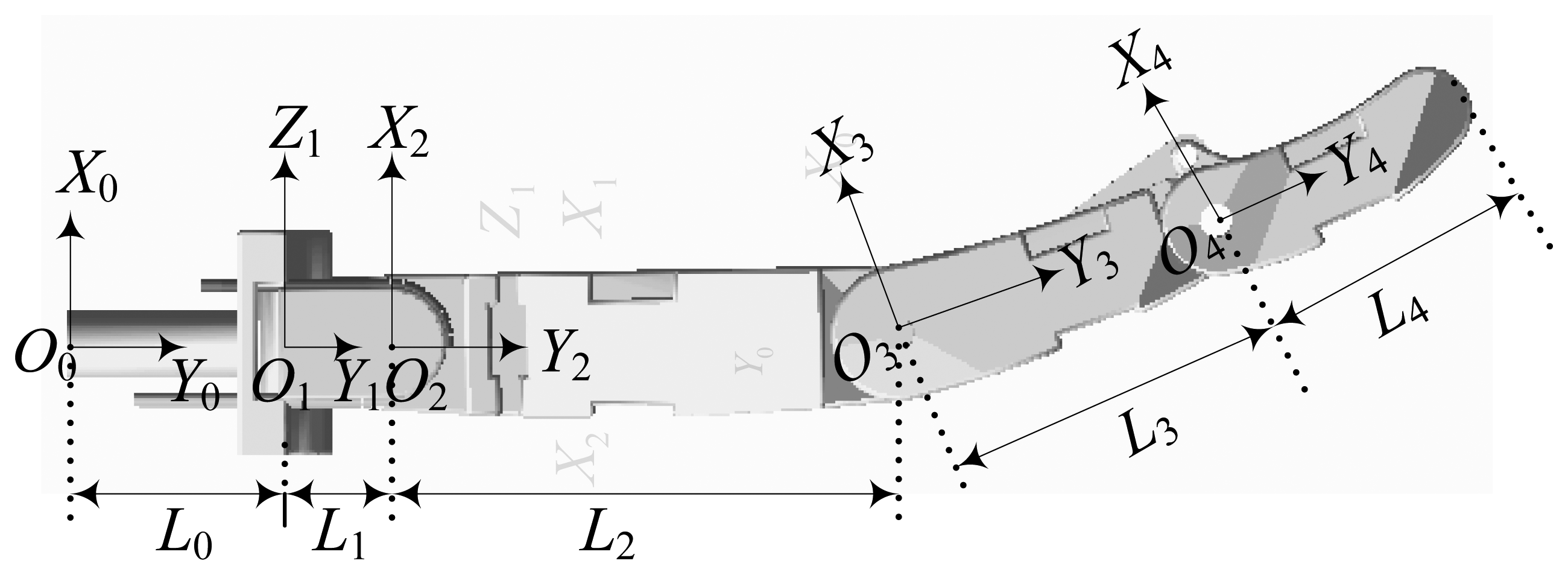
The Cartesian and joint coordinate systems are built, as show in Figure 7, where O₀ is the Cartesian coordinate system; O₁, O₂, O₃ and O₄ are respectively the coordinate system of each joint.

The Denavit-Hartenberg(D-H) parameters of the robot finger are listed in

Table 1. The D-H parameters of the robot finger.

i	ηi−1/(°)	Li−1/mm	di/mm	θi/rad
1	90.0	21	0	θ1
2	−90.0	9	0	θ2
3	0	45	0	θ3
4	0	30	0	θ4

.

where η_i−1 represents the rotation angle round Y_i−1 axis; L_i−1 is defined as the distance from Z_i−1 to Z_i; d_i is defined as the distance from Y_i-1 to Y_i.

According to Figure 7 and Table 1, the kinematics equation of the three-DOF finger is expressed as:

$$\mathit{A}={\mathit{A}}_1{\mathit{A}}_2{\mathit{A}}_3{\mathit{A}}_4{\mathit{A}}_5$$

(12)

where:

$$\begin{array}{cc}{\mathit{A}}_1=\left[\begin{array}{cccc}1& 0& 0& 0\\ 0& cos{\theta }_1& -sin{\theta }_1& L_0\\ 0& sin{\theta }_1& cos{\theta }_1& 0\\ 0& 0& 0& 1\end{array}\right]& {\mathit{A}}_2=\left[\begin{array}{cccc}cos{\theta }_2& -sin{\theta }_2& 0& 0\\ sin{\theta }_2& cos{\theta }_2& 0& L_1\\ 0& 0& 1& 0\\ 0& 0& 0& 1\end{array}\right]\\ {\mathit{A}}_3=\left[\begin{array}{cccc}cos{\theta }_3& -sin{\theta }_3& 0& 0\\ sin{\theta }_3& cos{\theta }_3& 0& L_2\\ 0& 0& 1& 0\\ 0& 0& 0& 1\end{array}\right]& {\mathit{A}}_4=\left[\begin{array}{cccc}cos{\theta }_4& -sin{\theta }_4& 0& 0\\ sin{\theta }_4& cos{\theta }_4& 0& L_3\\ 0& 0& 1& 0\\ 0& 0& 0& 1\end{array}\right]\\ {\mathit{A}}_5=\left[\begin{array}{cccc}1& 0& 0& 0\\ 0& 1& 0& L_4\\ 0& 0& 1& 0\\ 0& 0& 0& 1\end{array}\right]& \mathit{A}=\left[\begin{array}{cccc}{n}_x& o_x& a_x& x\\ n_y& o_y& a_y& y\\ n_z& o_z& a_z& z\\ 0& 0& 0& 1\end{array}\right]\end{array}$$

where x, y and z are the coordinate values of the fingertip in Cartesian coordinate system respectively.

The following equations can be obtained from Equation (12):

$$-ysin{\theta }_1+zcos{\theta }_1+L_{0}sin{\theta }_1=0$$

(13)

$${w_1}^2+{(w_2-L_2)}^2-2L_3(-w_{1}sin{\theta }_3+(w_2-L_2)cos{\theta }_3)+{L_3}^2={L_4}^2$$

(14)

$${(q_2-L_1)}^2+{q_1}^2-2((q_2-L_1)cos{\theta }_2-q_{1}sin{\theta }_2)L_2+{L_2}^2={L_4}^2+{L_3}^2+2L_4{L}_{3}cos{\theta }_4$$

(15)

$$m_{1}cos{\theta }_4+m_{2}sin{\theta }_4-L_{3}sin{\theta }_4=0$$

(16)

where:

$$\begin{array}{c}{q}_1=x,q_2=ycos{\theta }_1+zsin{\theta }_1-L_{1}cos{\theta }_1\\ w_1=q_{1}cos{\theta }_2+q_{2}sin{\theta }_2-L_{1}sin{\theta }_2\\ w_2=-q_{1}sin{\theta }_2+q_{2}cos{\theta }_2-L_{1}cos{\theta }_2\\ m_1=w_{1}cos{\theta }_3+w_{2}sin{\theta }_3-L_{2}sin{\theta }_3\\ m_2=-w_{1}sin{\theta }_3+w_{2}cos{\theta }_3-L_{2}cos{\theta }_3\end{array}$$

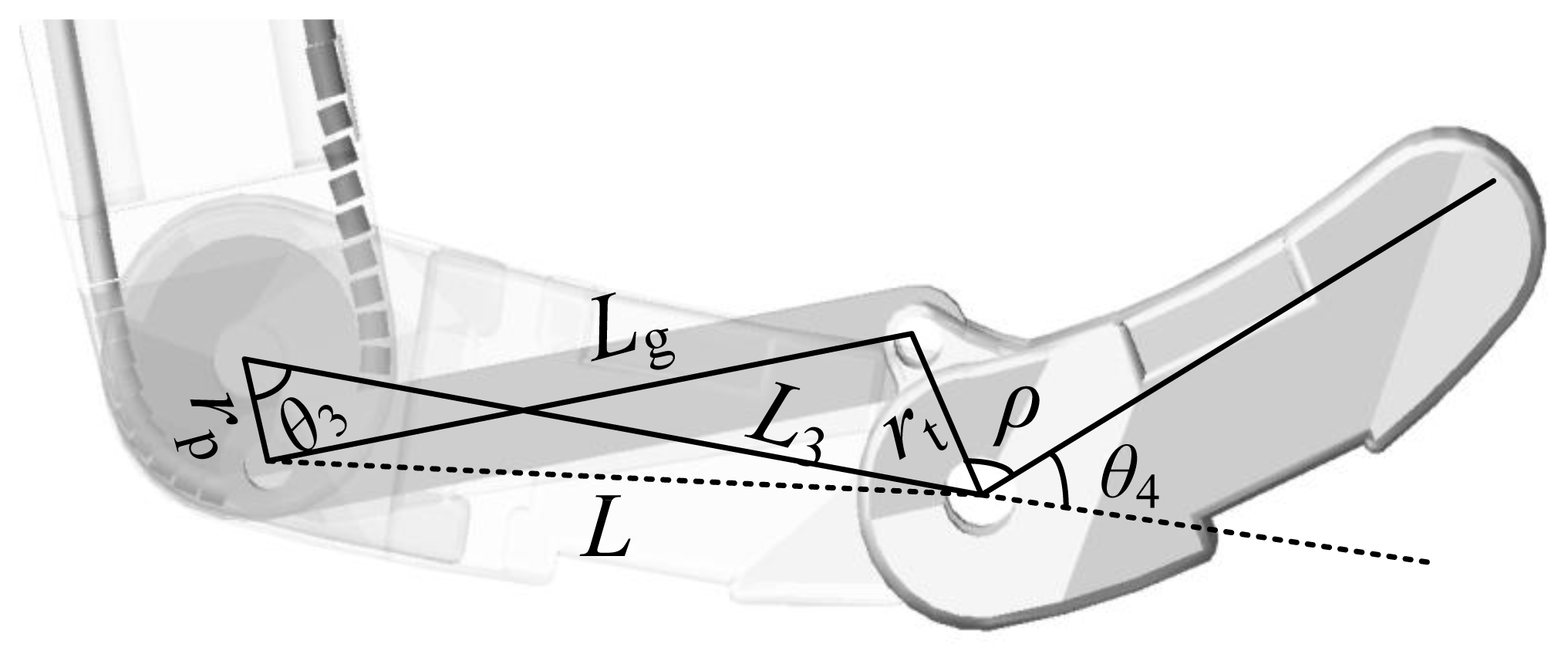
In addition, there is relationship between θ₃ and θ₄ due to the coupled structure, as shown in Figure 8.

The relational expressions between θ₃ and θ₄ are given by:

$$\begin{array}{c}L=\sqrt{{r_{\text{p}}}^2+{L_3}^2-2r_{\text{p}}{L}_{3}cos{\theta }_3}\\ \alpha =arcos(\frac{{r_t}^2+L^2-{L_g}^2}{2r_{t}L})\\ \beta =\alpha -arcos(\frac{L^2+{L_3}^2-{r_p}^2}{2L{L}_3})\\ {\theta }_4=\pi -\rho -\beta \end{array}$$

(17)

where ρ, r_p, L_g and r_t are constant, ρ = 1.52 rad, r_p = 4 mm, L_g = 27 mm, r_t = 6.2 mm.

It is easy to get the solution of θ₁ from Equation (13). However, Equations (14–17) are nonlinear and the computation cost is high, which is a limitation of inverse kinematics [16]. Therefore it is not easy to get the solutions of θ₂, θ₃ and θ₄. Since the control system is built in MATLAB, the fsovle function in MATLAB can be used to solve the nonlinear equations. The fsovle function solves the equations by the iterative method and hence the initial values of the iteration have a great influence on the simulation speed. Since the angular displacements are continuous, the current solutions can be used as the initial values of the next iteration.

3.4. The Position Controller

In order to control the position of the robot finger accurately, it is necessary to get the relationship between the joint angular displacements and the tendon displacements. Due to the particular design and neglecting the tendon elasticity, the relationship can be expressed as [9,10]:

$$\mathrm{\Delta }\mathit{l}={\mathit{R}}^{\text{T}}\mathrm{\Delta }\mathit{\theta }$$

(18)

where R is defined in Equation (3); Δl and Δθ are defined in Section 3.1.

4. Simulation and Analysis

4.1. Simulation Setups

The control system is built in MATLAB using the control module, as shown in Figure 9. The sample time of the simulation is 0.001 s. The simulation is mainly to validate the performance of the adaptive impedance control in uncertain environment and the reasonableness of the robot finger model. The impedance parameters and the adaptive parameters are given by:

$$\begin{array}{l}\begin{array}{lll}{\mathit{M}}_{\text{d}}=\left[\begin{array}{ccc}200& 0& 0\\ 0& 200& 0\\ 0& 0& 200\end{array}\right]\text{kg},\hfill & {\mathit{K}}_{\text{d}}=\left[\begin{array}{ccc}100& 0& 0\\ 0& 100& 0\\ 0& 0& 100\end{array}\right]\text{N}/\text{m},\hfill & {\mathit{B}}_{\text{d}}=\left[\begin{array}{ccc}3000& 0& 0\\ 0& 3000& 0\\ 0& 0& 3000\end{array}\right]N/(m/\text{s})\hfill \end{array}\hfill \\ {\sigma }_2=0.001,{\sigma }_1={\sigma }_3=0.09,{\alpha }_1={\beta }_1={\lambda }_1=0.1,{\omega }_p=0.27,{\omega }_v=0.25.\hfill \end{array}$$

4.2. The Position Control

In the free space, the finger motion is controlled by the position controller. The simulation time is set to 0.5 s. The final-desired angular displacements of the joints are [0, −0.17, −1.25]^T rad. Then the position controller controls the finger motion according to the desired trajectories. The results are shown in Figures 10, 11 and 12.

From Figures 10, 12 and 12, we may conclude that the actual angular displacements lag behind the desired one at the beginning. The reason is that the finger is driven by tendons which have elasticity and it takes some time for the tendons to go from slack to tight in the simulation. So, on the whole, the results are satisfactory.

4.3. Uncertainties in Environment Stiffness

Firstly, the robot finger is required to track on the environment which is a cylinder and has the stiffness of 10,000 N/m. The desired contact force is [−3, 6, 0]^T N. The fingertip makes contact with the environment at about 0.48 s, as shown in Figure 13. The force tracking results are shown in Figure 14.

In the next simulation, the environment stiffness is modified as 80,000 N/m and other conditions remain unchanged. After rerunning, the force tracking results are shown in Figure 15.

Figures 14 and 15 show that the average error of the force tracking is both less than 0.5 N in different stiffness although the actual force is oscillating due to the tendons, so on the whole, the force tracking results are satisfying when the environment stiffness is different, that is to say, without knowing the environment stiffness information, the force control algorithm performs well.

4.4. Uncertainties in Environment Position

In order to validate the robustness without knowing the environment position, let the environment position suddenly change at 0.65 s in the simulation. The change takes 0.005 s and the direction is shown in Figure 16. The displacement of the environment is 0.5 mm. The environment stiffness is 10,000 N/m and other conditions remain unchanged. The force tracking results are shown in Figure 17.

Comparing the force plot of Figure 17 with that of Figure 14 shows that the contact force changes at 0.65 s in Figure 17 due to the sudden change of environment position and the force overshoots are about 70% on x-direction and 65% on y-direction and the settling time is about 0.02 s. These demonstrate that without knowing the environment position information, the force control algorithm is robust.

Another simulation is carried out for the moving environment, as shown in Figure 18. The velocity of the environment movement is 0.025 m/s. There is dynamic friction between fingertip and environment due to the relative sliding. Hence, the desired force is set to [−3, 6, −1.88]^T N, where the force on z-direction is decided by friction coefficient. And the environment stiffness is also 10,000 N/m. The force tracking results are shown in Figure 19. Figure 19 shows that the environment movement has little impact on the force tracking results. This simulation demonstrates that the algorithm can perform diverse tasks.

5. Conclusions

In the joint simulation with ADAMS and MATLAB, the results of the position tracking and force tracking are satisfactory on the whole. In particular, the control system can keep the contact force near to expected value when the position or stiffness of the environment is uncertain, so the proposed adaptive impedance control algorithm is robust and the control system is suitable for a tendon-driven hand and the dexterous hand model built in ADAMS is reasonable. However, the tendon friction and joint friction are not considered in the robot hand model built in ADAMS. The friction can affect the control performance in practice, so the following research should build the friction model for the tendons and joints.

References

- Jung, S.; Hsia, T.C.; Bonitz, R.G. Force tracking impedance control of robot manipulators under unknown environment. IEEE Trans. Control Syst. Technol. 2004, 12, 474–483. [Google Scholar]
- Platt, R.; Abdallah, M.; Wampler, C. Multiple-Priority Impedance Control. Proceedings of the IEEE International Conference on Robotics and Automation, Shanghai, China, 9–13 May 2011; pp. 6033–6038.
- Jung, S.; Hsia, T.C. Force Tracking Impedance Control of Robot Manipulators for Environment with Damping. Proceedings of the 33rd Annual Conference of the IEEE Industrial Electronics Society, Taipei, Taiwan, 5–8 November 2007; pp. 2742–2747.
- Chen, Z.; Lii, N.Y.; Jin, M.; Fan, S.W.; Liu, H. Intelligent Robotics and Applications; Liu, H.H., Ding, H., Xiong, Z.H., Zhu, X.Y., Eds.; Springer Berlin Heidelberg: Berlin, Germany, 2010; pp. 1–12. [Google Scholar]
- Biagiotti, L.; Liu, H.; Hirzinger, G.; Melchiorri, C. Cartesian Impedance Control for Dexterous Manipulation. Proceedings of the 2003 IEEE/RSJ International Conference on Intelligent Robots and Systems, Las Vegas, NV, USA, 27–31 October 2003; pp. 3270–3275.
- Lasky, T.A.; Hsia, T.C. On Force-Tracking Impedance Control of Robot Manipulators. Proceedings of the 1991 IEEE International Conference on Robotics and Automation, Sacramento, CA, USA, 9–11 April 1991; pp. 274–280.
- Seraji, H. Adaptive Admittance Control: An Approach to Explicit Force Control in Compliant Motion. Proceedings of the 1994 IEEE International Conference on Robotics and Automation, San Diego, CA, USA, 8–13 May 1994; pp. 2705–2712.
- Diftler, M.A.; Mehling, J.S.; Abdallah, M.E.; Radford, N.A.; Bridgwater, L.B.; Sanders, A.M.; Askew, R.S.; Linn, D.M.; Yamokoski, J.D.; Permenter, F.A.; et al. Robonaut—The First Humanoid Robot in Space. Proceedings of the 2011 IEEE International Conference on Robotics and Automation, Shanghai, China, 9–13 May 2011; pp. 2178–2183.
- Abdallah, M.E.; Platt, R.; Wampler, C.W.; Hargrave, B. Applied Joint-Space Torque and Stiffness Control of Tendon-Driven Fingers. Proceedings of the 10th IEEE-RAS International Conference on Humanoid Robots (Humanoids), Nashville, TN, USA, 6–8 December 2010; pp. 74–79.
- Borghesan, G.; Palli, G.; Melchiorri, C. Design of Tendon-Driven Robotic Fingers: Modeling and Control Issues. Proceedings of the 2010 IEEE International Conference on Robotics and Automation, Anchorage, AK, USA, 3–7 May 2010; pp. 793–798.
- Li, H.J.; Yang, Z.J. Study on the modelling for wire rope substances in Adams. Mech. Manag. Dev. 2007, 4, 4–5. [Google Scholar]
- Li, J.W.; Bu, C.G.; Wang, L. The application of Macro command in ADAMS in building the virtual prototype of cable drill. Mach. Tool Hydraul. 2011, 39, 150–153. [Google Scholar]
- Heinrichs, B.; Sepehri, N.; Thornton-Trump, A.B. Position-based impedance control of an industrial hydraulic manipulator. IEEE Control Syst. 1997, 17, 46–52. [Google Scholar]
- Sadjadian, H.; Taghiradf, H.D. Impedance Control of the Hydraulic Shoulder a 3-DOF Parallel Manipulator. Proceedings of the IEEE International Conference on Robotics and Biomimetics, Kunming, China, 17–20 December 2006; pp. 526–531.
- Ioannou, P.A.; Kokotovic, P.V. Adaptive systems with reduced models. Lect. Notes Control Inf. Sci. 1983, 47, 162. [Google Scholar]
- Escande, A.; Mansard, N.; Wieber, P.B. Fast Resolution of Hierarchized Inverse Kinematics with Inequality Constraints. Proceedings of the 2010 IEEE International Conference on Robotics and Automation, Anchorage, AK, USA, 3–7 May 2010; pp. 3733–3738.